Products of Farey Fractions

Abstract.

The Farey fractions ${\mathcal{F}}_{n}$ of order $n$ consist of all fractions $\frac{h}{k}$i lying in the closed unit interval and having denominator at most $n$. in the unit interval with denominator at most $n$, not necessarily in lowest terms. This paper considers the products $F_{n}$ of all nonzero Farey fractions of order $n$. It studies their growth and their divisibility properties by powers of a fixed prime, given by ${\rm ord}_{p}(F_{n})$, as a function of $n$. It presents evidence suggesting that information related to the Riemann hypothesis may be encoded in functions related to ${\rm ord}_{p}(F_{n})$ for a single fixed prime $p$. This encoding makes use of a relation of these products to the products $G_{n}$ of all reduced and unreduced Farey fractions of order $n$, which are connected by Möbius inversion. It introduces new arithmetic functions which mix the Möbius function with functions of radix expansions to a fixed prime base $p$.

1. Introduction

The Farey sequence ${\mathcal{F}}_{n}$ of order $n$ is the sequence of reduced fractions $\frac{h}{k}$ between $0$ and $1$ (including $0$ and $1$) which, when in lowest terms, have denominators less than or equal to $n$, arranged in order of increasing size. We write it as

$${\mathcal{F}}_{n}:=\{\frac{h}{k}:0\leq h\leq k\leq n:\,gcd(h,k)=1.\}$$

Farey sequences are important in studying Diophantine approximation properties of real numbers, cf. Hardy and Wright [7, Chap. III]. They can be viewed as additive objects that encode deep arithmetic properties of both integers and the rational numbers.

The set of Farey fractions ${\mathcal{F}}_{n}$ is known to approximate the uniform distribution on the unit interval $[0,1]$ as $n\to\infty$, viewing it as defining a measure given by a sum of (normalized) delta functions at the points of ${\mathcal{F}}_{n}$. The rate at which these measures approach the uniform distribution can be related to the Riemann hypothesis. A precise version is given in a celebrated theorem of Franel [5], with extensions made in many later works, including Landau [16], Mikolás [18], [19], Huxley [8, Chap. 9], and Kanemitsu and Yoshimoto [11], [12].

1.1. Farey products

We consider a multiplicative statistic associated to the Farey fractions–the products of the nonzero elements of the Farey sequence, termed Farey products. To study Farey products we use the positive Farey sequence

$${\mathcal{F}}_{n}^{\ast}:={\mathcal{F}}_{n}\smallsetminus\{0\}=\{\frac{h}{k}:1\leq h\leq k\leq n:\,gcd(h,k)=1\}.$$

For example, we have

$${\mathcal{F}}_{4}^{\ast}:=\left\{\frac{1}{4},\frac{1}{3},\frac{1}{2},\frac{2}{3},\frac{3}{4},\frac{1}{1}\right\}.$$

We let $\Phi(n)=|{\mathcal{F}}_{n}^{\ast}|$ denote the number of elements of ${\mathcal{F}}_{n}^{\ast}$, and we clearly have:

$$\Phi(n)=\sum_{k=1}^{n}\varphi(k),$$ (1.1)

where $\varphi(k)$ denotes the Euler totient function, which has

$$\varphi(k)=|({\mathbb{Z}}/k{\mathbb{Z}})^{\times}|=|\{a:1\leq a\leq k\,\mbox{with}\,\gcd(a,k)=1\}|.$$

To describe the ordered Farey fractions we introduce the notation $\rho_{r}=\rho_{r,n}$ for the $r$-th fraction in the ordered sequence $\rho_{r,n}<\rho_{r+1,n}$, writing

$${\mathcal{F}}_{n}^{\ast}=\{\rho_{r}=\rho_{r,n}:1\leq r\leq\Phi(n)\}.$$

The product of the Farey fractions is then

$$F_{n}:=\prod_{r=1}^{\Phi(n)}\rho_{r,n}=\frac{N_{n}}{D_{n}},$$ (1.2)

in which $N_{n}$ denotes the product of the numerators of all the $\rho_{r,n}$ and $D_{n}$ the product of their denominators; here $N_{n}/D_{n}$ is not in lowest terms for $n>2$, cf. Section 4.6. The Farey product $F_{n}$ is a rational number in the unit interval that rapidly gets small as $n$ increases.

It proves convenient to introduce the reciprocal Farey products

$$\overline{F}_{n}:=\frac{1}{F_{n}}=\frac{D_{n}}{N_{n}}=\Big{(}\prod_{r=1}^{\Phi(n)}\rho_{r}\Big{)}^{-1},$$ (1.3)

to facilitate comparison with other results ([14]) ; the values of $\overline{F}_{n}$ rapidly increase with $n$. Clearly $\overline{F}_{n}\geq 1$ and we find that $\overline{F}_{1}=1,\overline{F}_{2}=2,\overline{F}_{3}=9,\overline{F}_{4}=48,\overline{F}_{5}=1250,\overline{F}_{6}=9000$. In these examples $\gcd(N_{n},D_{n})$ becomes large, such that $\overline{F}_{n}$ is an integer for small $n$. However $\overline{F}_{7}=\frac{3\cdot 5^{2}\cdot 7^{6}}{2}$ is not an integer, and it is known that only finitely many $\overline{F}_{n}$ are integers, see Section 4.4.

Reciprocal Farey products have the following interesting features.

1. The statistic $\overline{F}_{n}$ extracts a single rational number from the whole collection of Farey fractions ${\mathcal{F}}_{n}^{\ast}$. The growth behavior of the numbers $\overline{F}_{n}$ encodes the Riemann hypothesis, as a consequence of a 1951 result of Mikolás [19] presented in Section 3.1. This encoding concerns the size of an error term in an approximation of $\log\overline{F}_{n}$ in which the main term is an arithmetic function related to both the Euler totient function and the von Mangoldt function.

2. The functions ${\nu}_{p}(\overline{F}_{n})={\rm ord}_{p}(\overline{F}_{n})$ that describe divisibility of $\overline{F}_{n}$ by a (positive or negative) power of a fixed prime $p$, have an interesting structure. Here ${\rm ord}_{p}(\overline{F}_{n})$ gives the exact (positive or negative or zero) power of $p$ dividing $\overline{F}_{n}$, so that $p^{-{\rm ord}_{p}(\overline{F}_{n})}\overline{F}_{n}$ is a rational number having both numerator and denominator prime to $p$, and $||\overline{F}_{n}||_{p}=p^{-{\rm ord}_{p}(\overline{F}_{n})}$ is the usual $p$-adic valuation of $\overline{F}_{n}$. There is generally a large cancellation of powers of $p$ in the numerator and denominator of the product defining $\overline{F}_{n}$, and the behavior of this cancellation is of interest.

Since reciprocal Farey products encode the Riemann hypothesis we may expect in advance that they will exhibit complicated and mysterious arithmetic behavior. Even simple-looking questions may prove to be quite difficult.

1.2. Results

We study the size of the rational numbers $\overline{F}_{n}$ at the real place measured using a logarithmic scale by

$${\nu}_{\infty}(\overline{F}_{n}):=\log(\overline{F}_{n}).$$ (1.4)

For each prime $p$, we study the functions

$${\nu}_{p}(\overline{F}_{n}):={\rm ord}_{p}(\overline{F}_{n})$$ (1.5)

which measure the $p$-divisibility of $\overline{F}_{n}$; the values ${\rm ord}_{p}(\overline{F}_{n})$ may be positive or negative.

The investigations of this paper first obtain information on Farey products $F_{n}$ as they relate to the products of all reduced and unreduced Farey fractions $G_{n}$, which we term unreduced Farey products. The reciprocal unreduced Farey products $\overline{G}_{n}=1/G_{n}$ are always integers, equal to the product of all binomial coefficients in the $n$-row of Pascal’s triangle.

In Section 2 we study the reciprocal unreduced Farey products $\overline{G}_{n}$, first summarizing some results taken from our paper [14]. The function $\log(\overline{G}_{n})$ has a smooth growth given by an asymptotic expansion valid to all orders of $\frac{1}{n^{k}}$. The functions ${\rm ord}_{p}(\overline{G}_{n})$ have a complicated but analyzable behavior related to the base $p$ radix expansions of the integers from $1$ to $n$. One also has $0\leq{\rm ord}_{p}(\overline{G}_{n})<n\log_{p}n$. Then in Section 2.2 we give basic relations between $\overline{F}_{n}$ and $\overline{G}_{n}$ which involve the floor function. These start with the product relation

$$\overline{G}_{n}=\prod_{\ell=1}^{n}\overline{F}_{[n/\ell]},$$

and by Möbius inversion we obtain the basic identity

$$\overline{F}_{n}=\prod_{\ell=1}^{n}(\overline{G}_{[n/\ell]})^{\mu(\ell)}.$$

We obtain further formulas by splitting the sums using a parameter $L$ related to the Dirichlet hyperbola method, as formulated in Diamond [4, Lemma 3.1].

In Section 3 we turn to $\overline{F}_{n}$ and study the growth rate of $\log(\overline{F}_{n})$. This function does not have a complete asymptotic expansion in terms of simple functions. We review known results of Mikolás which relate fluctuations of this growth rate to the Riemann hypothesis. They say that $\log(\overline{F}_{n})$ is well approximated by a main term $\Phi(n)-\frac{1}{2}\psi(n)$, in which $\Phi(n)$ is as defined in (1.1), $\psi(n)=\sum_{k\leq n}\Lambda(k)$, with $\Lambda(n)$ being the von Mangoldt function. The size of the remainder term $R_{\overline{F}}(n)=\log(\overline{F}_{n})-\big{(}\Phi(n)-\frac{1}{2}\psi(n)\big{)}$ is then related to the Riemann hypothesis. In Section 3 we also review known results about the fluctuating behavior of $\Phi(n)$.

In Section 4 we study the functions ${\rm ord}_{p}(\overline{F}_{n})$. These functions have a more complicated behavior than of ${\rm ord}_{p}(\overline{G}_{n})$. We give formulas for computing ${\rm ord}_{p}(\overline{F}_{n})$, and present experimental data on its values for small primes $p$. We do not understand the behavior of ${\rm ord}_{p}(\overline{F}_{n})$ well theoretically, and our data leads us to formulate a set of four hypotheses stating (unproved) properties (P1) - (P4) that these functions might have. These hypothetical properties (P1) - (P4) include assertions that ${\rm ord}_{p}(\overline{F}_{n})$ has infinitely many sign changes; that a sign change always occurs between $n=p^{k}-1$ and $n=p^{k}$, for $k>1$; and that the growth rate of ${\rm ord}_{p}(\overline{F}_{n})$ is of order $O(n\log_{p}n)$. Even very special cases of these properties are unsolved problems which may be hard. For example: Is it true that for a prime $p$ the inequality ${\rm ord}_{p}(\overline{F}_{p^{2}-1})\leq 0$ always holds? This assertion comprises a family of one-sided inequalities involving Möbius function sums. A family of one-sided inequalities of this sort, if true, would be of great interest as providing fundamental new arithmetic information about the Möbius function. At the end of Section 4 we present a few theoretical results supporting the possible validity of these properties. We show that for each $p$ there is at least one sign change in the value of ${\rm ord}_{p}(\overline{F}_{n})$. Concerning the size of ${\rm ord}_{p}(\overline{F}_{n})$ we have the easy bound $|{\rm ord}_{p}(\overline{F}_{n})|\leq n(\log_{p}n)^{2}$ which follows from knowledge of ${\rm ord}_{p}(\overline{G}_{n})$.

In Section 5 we study relations between the growth rate of $\log(\overline{F}_{n})$ and the Riemann hypothesis, given by the result of Mikolás, with the main term in Mikolás formula being $\Phi(n)-\frac{1}{2}\psi(n)$. In this section we relate this main term to a quantity given entirely in terms of $\log(\overline{G}_{n})$ and the Möbius function, using a parallel with the “hyperbola method” of Dirichlet. In Section 5.2 we justify our definition of “replacement main term” $\Phi_{\infty}(n)$ by showing that the Riemann hypothesis implies that it is indeed close to the “main term” $\Phi(n)-\frac{1}{2}\psi(n)$ in the Mikolás formulation of the Riemann hypothesis. We obtain a formula for the “replacement remainder term” and present empirical evidence about its behavior. It has a very striking non-random features in which the influence of the Möbius function is clearly visible.

In Section 6, we ask: Can one approach the Riemann hypothesis through knowledge of the function ${\rm ord}_{p}(\overline{F}_{n})$ at a single fixed prime $p$? Note that the product formula for rational numbers expresses $\log(\overline{F}_{n})$ as a weighted sum of ${\rm ord}_{p}(\overline{F}_{n})$ for $p\leq n$, and by the Mikolás result this in principle allows the Riemann hypothesis to be expressed as a complicated function of all the functions ${\rm ord}_{p}(\overline{F}_{n})$ with variable $p$. Speculation that the Riemann hypothesis might be visible from data at a single prime $p$ seems initially unbelievable. It becomes less far-fetched when one observes from the formulas that the full set of Möbius function values $\{\mu(m):n\geq m\geq 1\}$ influence the values ${\rm ord}_{p}(\overline{F}_{n})$.

Section 6 parallels the recipe of Section 5 in formulating at the prime $p$ formulas analogous to the “replacement main term”, given now in terms of ${\rm ord}_{p}(\overline{G}_{n})$, which might serve as a “main term” to approximate the function ${\rm ord}_{p}(\overline{F}_{n})$. The new “replacement main terms” and “remainder terms” are based on the Möbius inversion relation between ${\rm ord}_{p}(\overline{F}_{n})$ and the ${\rm ord}_{p}(\overline{G}_{n})$, and the resulting division into two terms is related to the Dirichlet hyperbola method. For a fixed $p$ there are now three different possible recipes to split off a “main term” and “remainder term”, unlike the archimedean case considered in Section 5. The resulting terms include new kinds of arithmetic sums not studied before: individual terms in these sums involve Möbius function values multiplied by sums of the base $p$ digits at selected integer values. These new “replacement main terms” themselves have unusual structure, being oscillatory functions. However, after they are removed, one can ask the question whether the size of the “remainder terms” in these new expressions is related to zeta zeros, and in particular to the Riemann hypothesis.

We try all three for a “replacement main term”, and find experimentally that one of them gives plots of the remainder term having non-random features in striking parallel with the experimental data in the archimedean case in Section 5. This observation was a remarkable experimental discovery of this work.

In the final Section 7 we make concluding remarks on this possible encoding of the Riemann hypothesis at a fixed finite prime.

In Appendix A (Appendix A: Empirical Results for $p=3$ we present additional computational results for $p=3$ complementing results for $p=2$ given in Section 4.3.

2. Unreduced Farey Products

Unreduced Farey products provide an approach to understand the Farey products. The unreduced Farey sequence ${\mathcal{G}}_{n}$ is the ordered sequence of all reduced and unreduced fractions between $0$ and $1$ with denominator of size at most $n$, and its positive analogue, which we denote

$${\mathcal{G}}_{n}^{\ast}:=\left\{\frac{h}{k}:1\leq h\leq k\leq n\right\}.$$

We order these unreduced fractions in increasing order, breaking ties between equal fractions by placing them in order of increasing denominator. For example, we have

$${\mathcal{G}}_{4}^{\ast}:=\left\{\frac{1}{4},\frac{1}{3},\frac{1}{2},\frac{2}{4},\frac{2}{3},\frac{3}{4},\frac{1}{1},\frac{2}{2},\frac{3}{3},\frac{4}{4}\right\}.$$

Denoting the number of elements in ${\mathcal{G}}_{n}^{\ast}$ as $\Phi^{\ast}(n)$, we may may label the fractions in ${\mathcal{G}}_{n}^{\ast}$ in order as $\rho_{r}^{*}=\rho_{r,n}^{\ast}$ and write

$${\mathcal{G}}_{n}^{\ast}=\{\rho_{r}^{*}=\rho_{r,n}^{*}:1\leq r\leq\Phi^{\ast}(n)\}.$$

Here we have

$$\Phi^{\ast}(n)=\sum_{k=1}^{n}k={{n+1}\choose{2}}.$$ (2.1)

Now we define the unreduced Farey product

$$G_{n}:=\prod_{r=1}^{\Phi^{\ast}(n)}\rho_{r,n}^{\ast}=\frac{N_{n}^{\ast}}{D_{n}^{\ast}},$$

where $N_{n}^{\ast}$ denotes the product of the numerators of all $\rho_{r,n}^{\ast}$ and $D_{n}^{\ast}$ the corresponding product of denominators; certainly $N_{n}^{\ast}/D_{n}^{\ast}$ is not in lowest terms. Now we define the reciprocal unreduced Farey product

$$\overline{G}_{n}:=\frac{1}{G_{n}}=\frac{D_{n}^{\ast}}{N_{n}^{\ast}}=\Big{(}\prod_{r=1}^{\Phi_{n}^{\ast}}\rho_{r}\Big{)}^{-1}.$$

Here $\overline{G}_{1}=1,\overline{G}_{2}=2,\overline{G}_{3}=9,\overline{G}_{4}=96,\overline{G}_{5}=2500,\overline{G}_{6}=162000$ and $\overline{G}_{7}=3^{2}\cdot 5^{2}\cdot 7^{6}$ is an integer.

2.1. Properties of reciprocal unreduced Farey products $\overline{G}_{n}$

This section recalls results from a detailed study of reciprocal unreduced Farey products $\overline{G}_{n}$ made in [14]. from which we recall the following results. A first result is that $\overline{G}_{n}$ is always an integer, being given as a product of binomial coefficients

$$\overline{G}_{n}=\prod_{j=0}^{n}{{n}\choose{j}}.$$ (2.2)

For this reason the $\overline{G}_{n}$ are called binomial products in [14, Theorem 2.1]. The numerators and denominators in this formula have asymptotic expansions which when combined yield a good asymptotic expansion for $\log(\overline{G}_{n})$, valid when $n$ is a positive integer ([14, Theorem 3.1, Appendix A]).

Theorem 2.1.

For positive integers $n\to\infty$ there holds

$$\log(\overline{G}_{n})=\frac{1}{2}n^{2}-\frac{1}{2}n\log n+(1-\log(\sqrt{2\pi}))\,n-\frac{1}{3}\log n+g_{0}+O(\frac{1}{n}).$$ (2.3)

In this formula $g_{0}=-\frac{1}{2}\log(2\pi)-\frac{1}{12}+2\log A$ with $A$ denoting the Glaisher-Kinkelin constant $A=\exp\big{(}\frac{1}{12}-\zeta^{{}^{\prime}}(-1)\big{)}\approx 1.282427$.

One may extend $\overline{G}_{n}$ to a function of a real variable $x$ as a step function $\overline{G}_{x}:=\overline{G}_{\lfloor x\rfloor}$. When this is done, the asymptotic expansion (2.3) above remains valid only at integer values of $x$; the jumps in the step function are of size $\geq n$, which is larger than all but the first three terms in the expansion (2.3). For later use, we restate this in the form

$$\log(\overline{G}_{n})=\Phi^{\ast}(n)-\frac{1}{2}n\log n+\frac{1}{2}\log(\frac{e}{2\pi})\,n+O(\log n).$$ (2.4)

Secondly we have essentially sharp upper and lower bounds for ${\rm ord}_{p}(\overline{G}_{n})$ ([14, Theorems 6.7 and 6.8]).

Theorem 2.2.

For each prime $p$, there holds for all $n\geq 1$,

$$0\leq{\rm ord}_{p}(\overline{G}_{n})<n\log_{p}n.$$ (2.5)

The value at $n=p^{k}-1$ is ${\rm ord}_{p}(G_{p^{k}-1})=0$. The value at $n=p^{k}$ is

$${\rm ord}_{p}(\overline{G}_{p^{k}})=\left(kp^{k}-\frac{p^{k}-1}{p-1}\right).$$ (2.6)

This value has ${\rm ord}_{p}(\overline{G}_{n})\geq n\log_{p}n-n$.

We record next an explicit formula for ${\rm ord}_{p}(\overline{G}_{n})$, which is related to the base $p$ expansion of $n$. We write a positive integer $n$ in a general radix base $b\geq 2$ as

$$n:=\sum_{i=0}^{k}a_{i}b^{i},\,\mbox{for}\,b^{k}\leq n<b^{k+1}.$$

with digits $0\leq a_{i}=a_{i}(n)\leq b-1$ and $k=\lfloor\log_{b}n\rfloor.$

The sum of digits function (to base $b$) of $n$ is

$${d}_{b}(n):=\sum_{i=0}^{k}a_{i}(n),$$ (2.7)

The total digit summatory function (to base $b$) is

$${S}_{b}(n):=\sum_{j=0}^{n-1}{d}_{b}(j).$$ (2.8)

Then we have ([14, Theorem 5.1])

Theorem 2.3.

Let the prime $p$ be fixed. Then for all $n\geq 1$,

$${\nu}_{p}(\overline{G}_{n})={\rm ord}_{p}(\overline{G}_{n})=\frac{1}{p-1}\Big{(}2{S}_{p}(n)-(n-1){d}_{p}(n)\Big{)}.$$ (2.9)

This identity was established starting from an observation made in Granville [6, equation (18)]. There is an explicit expression for ${S}_{p}(n)$ due to Delange [1], which applies more generally to radix expansions to an arbitrary integer base $b\geq 2$.

Theorem 2.4.

(Delange (1975)) Given an integer base $b\geq 2$, there exists a function ${f}_{b}(x)$ on the real line, which is continuous and periodic of period $1$, such that for all integers $n\geq 1$,

$${S}_{b}(n)=\left(\frac{b-1}{2}\right)n\log_{b}n+{f}_{b}(\log_{b}n)n.$$ (2.10)

Delange showed that the function ${f}_{b}(x)$ has a Fourier series expansion

$${f}_{b}(x)=\sum_{k\in{\mathbb{Z}}}c_{b}(k)e^{2\pi ikx}$$

whose Fourier coefficients are given for $k\neq 0$ by

$$c_{b}(k)=-\frac{b-1}{2k\pi i}\left(1+\frac{2k\pi i}{\log b}\right)^{-1}\zeta\left(\frac{2k\pi i}{\log b}\right).$$ (2.11)

with $\zeta(s)$ being the Riemann zeta function, and with constant term

$$c_{b}(0)=\frac{b-1}{2\log(b)}(\log(2\pi)-1)-\left(\frac{b+1}{4}\right).$$ (2.12)

The function ${f}_{b}(x)$ is continuous but Delange [1, Sect. 3] showed it is everywhere non-differentiable, see also Tenenbaum [22].

To illustrate the behavior of ${\rm ord}_{p}(\overline{G}_{n})$ which is described by Theorem 2.3 and 2.4, in Figure 2.1 we give a plot of ${\rm ord}_{2}(\overline{G}_{n})$ for $1\leq n\leq 1023=2^{10}-1$. The visible “streaks” in the plot represent values where ${d}_{p}(n)=j$ has a constant value. There are large jumps in ${\rm ord}_{2}(\overline{G}_{n})$ between the value $n=2^{k}-1$ where ${\rm ord}_{2}(\overline{G}_{n})=0$, and $n=2^{k}$, where ${\rm ord}_{2}(\overline{G}_{n})\geq(k-1)n.$

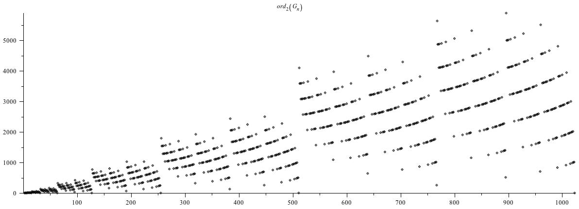
Figure 2.1. ${\rm ord}_{2}(\overline{G}_{n})$, $1\leq n\leq 1023$.

In Figure 2.2 we plot the behavior of $\frac{1}{n}{\rm ord}_{2}(\overline{G}_{n})$ over the range of a single power of $2$, $2^{k}\leq n\leq 2^{k+1}-1$, sorted in order of increasing size. The sorted values of $\frac{1}{n}{\rm ord}_{2}(\overline{G}_{n})$ over this range have mean about $\frac{1}{2}k=\frac{1}{2}\log_{2}n$ as $k\to\infty$, have variance proportional to $\sqrt{\log n})$, and if properly scaled satisfies a central limit theorem as $k\to\infty$.

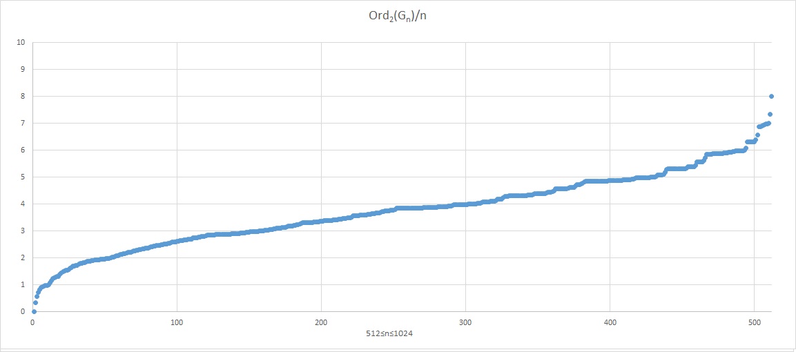
Figure 2.2. Sorted values of $\frac{1}{n}{\rm ord}_{2}(\overline{G}_{n})$, $512\leq n\leq 1024$.

These two plots of ${\rm ord}_{2}(\overline{G}_{n})$ are presented for later comparison with ${\rm ord}_{2}(\overline{F}_{n})$.

2.2. Relation of the $\overline{F}_{n}$ and $\overline{G}_{n}$: Möbius inversion

The reciprocal Farey products $\overline{F}_{n}$ are directly expressible in terms of reciprocal unreduced Farey products $\overline{G}_{n}$ introduced in [14] by Möbius inversion.

Theorem 2.5.

The reciprocal unreduced Farey products are related to the reciprocal Farey products by the identity

$$\overline{G}_{n}=\prod_{\ell=1}^{n}\overline{F}_{\lfloor n/\ell\rfloor}.$$ (2.13)

By Möbius inversion, there holds

$$\overline{F}_{n}=\prod_{\ell=1}^{n}\big{(}\overline{G}_{\lfloor n/\ell\rfloor}\big{)}^{\mu(\ell)}.$$ (2.14)

Proof.

We group the elements $\frac{h}{k}$of ${\mathcal{G}}_{n}^{\ast}$ according to the value $\ell:=\gcd(h,k)$. The fractions with a fixed $\ell$ are in one-to-one correspondence with elements of the Farey sequence ${\mathcal{F}}_{n/\ell}$, and their product is identical with the product of the elements of that Farey sequence. This gives the first formula.

To obtain the second formula, we make a detour by taking a logarithm to obtain an additive formula, namely

$$\log(\overline{G}_{n})=\sum_{\ell=1}^{n}\,\log(\overline{F}_{\lfloor n/\ell}\rfloor),$$ (2.15)

A variant of the Möbius inversion formula ([21, Sec. I.2, Theorem 9]) then yields

$$\log(\overline{F}_{n})=\sum_{\ell=1}^{n}\mu(\ell)\,\log(\overline{G}_{\lfloor n/\ell\rfloor}).$$ (2.16)

The second formula follows by exponentiating both sides of (2.16). ∎

Remark 2.6.

If we define $\overline{G}_{x}=\overline{G}_{\lfloor x\rfloor}$ and $\overline{F}_{x}=\overline{F}_{\lfloor x\rfloor}$ as step functions of a real variable $x$ then we can rewrite the formulas above without the floor function notation, as

$$\overline{G}_{n}=\prod_{\ell=1}^{n}\overline{F}_{n/\ell}\quad\mbox{and}\quad\overline{F}_{n}=\prod_{\ell=1}^{n}\big{(}\overline{G}_{n/\ell}\big{)}^{\mu(\ell)}.$$

However the subtleties in the behavior of these functions certainly has to do with the floor function, and we prefer to have it visible.

In the formulas of Theorem 2.5 the fractions $\lfloor n/\ell\rfloor$ take only about $2\sqrt{n}$ distinct values. This allows the possibility to combine terms in the sum and take advantage of cancellation in sums of the Möbius function. We recall that the Mertens function $M(n)$ is defined by

$$M(n):=\sum_{j=1}^{n}\mu(j).$$ (2.17)

We split the sum (2.16) for $\log(\overline{F}_{n})$ into two parts, using a parameter $L$, as

$$\log(\overline{F}_{n}) = \sum_{k=1}^{n/(L+1)}\mu(k)\log(\overline{G}_{\lfloor n/k\rfloor})+\sum_{\ell=1}^{L}\left(\sum_{\frac{n}{\ell+1}<k\leq\frac{n}{\ell}}\mu(k)\right)\log(\overline{G}_{\ell})\,$$

$$= \sum_{k=1}^{n/(L+1)}\mu(k)\log(\overline{G}_{\lfloor n/k\rfloor})+\sum_{\ell=1}^{L}\left(M\left(\frac{n}{\ell}\right)-M\left(\frac{n}{\ell+1}\right)\right)\log(\overline{G}_{\ell}).$$

The second term accumulates cancellations among consecutive Möbius function values. This sort of splitting formula is associated with the Dirichlet hyperbola method, as formulated in Diamond [4, Lemma 2.1], cf. Tenenbaum [21, Sect. 3.2].

The most balanced parameter choice is $L=\lfloor\sqrt{n}\rfloor$, in which case we write

$$\log(\overline{F}_{n})=\Phi_{\infty}^{+}(n)+\Phi_{\infty}^{-}(n),$$ (2.18)

setting

$$\Phi_{\infty}^{+}(n):=\sum_{k=1}^{n/(\lfloor\sqrt{n}\rfloor+1)}\mu(k)\log(\overline{G}_{\lfloor n/k\rfloor})$$ (2.19)

and

$$\Phi_{\infty}^{-}(n):=\sum_{\ell=1}^{\lfloor\sqrt{n}\rfloor}\left(M\left(\frac{n}{\ell}\right)-M(n/(\ell+1))\right)\log(\overline{G}_{\ell}).$$ (2.20)

Note that if $m^{2}\leq n<(m+1)^{2}$ then

$$\frac{n}{(\lfloor\sqrt{n}\rfloor+1)}=\begin{cases}\lfloor\sqrt{n}\rfloor-1&\quad\mbox{if}\quad m^{2}\leq n<m(m+1)\\ \lfloor\sqrt{n}\rfloor&\quad\mbox{if}\quad m(m+1)\leq n<(m+1)^{2}.\end{cases}$$

It is well known that the Riemann hypothesis is equivalent to the growth estimate $M(n)=O(n^{\frac{1}{2}+\epsilon})$ being valid for each $\epsilon>0,$ see Titchmarsh [23, Theorem 14.25 (C)]. To obtain some unconditional cancellations in the second sum, one may take $L$ to be much smaller, e.g. $L=\exp((\log n)^{\theta})$ for a suitable choice of $\theta$, and use the unconditional estimate $M(n)=O(n\exp(-(\log n)^{\theta}))$ known to be valid for $\theta>\frac{3}{5}$. To extract information from the resulting formulas seems to require additional ideas, which we hope to address on another occasion.

Remark 2.7.

Parallel to (2.15) and (2.16) for $\log\overline{G}_{n}$ and $\log\overline{F}_{n}$ there are analogous formulas for prime divisibility of $\overline{G}_{n}$ and $\overline{F}_{n}$. Applying ${\rm ord}_{p}(\cdot)$ in Theorem 2.5 yields

$${\rm ord}_{p}(\overline{G}_{n})=\sum_{\ell=1}^{n}{\rm ord}_{p}(\overline{F}_{\lfloor n/\ell\rfloor}),$$ (2.21)

and

$${\rm ord}_{p}(\overline{F}_{n})=\sum_{\ell=1}^{n}\mu(\ell)\,{\rm ord}_{p}(\overline{G}_{\lfloor n/\ell\rfloor}).$$ (2.22)

We can also split these sums into two parts using a parameter $L$, as done above.

3. Reciprocal Farey Product $\overline{F}_{n}$ Archimedean Growth Rate

The growth rate of Farey products measured by $\log(\overline{F}_{n})$ was studied by Mikolás [19], who showed their behavior encodes the Riemann hypothesis. We describe this result and other known results about its oscillatory main term.

3.1. Mikolás’s theorem

In 1951 Mikolás obtained an asymptotic formula for the growth rate of $\log(\overline{F}_{n})$ having an error term related to the Riemann hypothesis. To formulate his results, we first recall that, for $Re(s)>1$, there holds

$$\frac{\zeta^{\prime}(s)}{\zeta(s)}=-\sum_{n=1}^{\infty}\Lambda(n)n^{-s},$$ (3.1)

where the von Mangoldt function $\Lambda(n)$ has

$$\Lambda(n)=\left\{\begin{array}[]{ll}\log\,p&\mbox{if}\,\,\,n=p^{k},\\ 0&\mbox{if}\,\,\,n\neq p^{k}.\end{array}\right.$$

We define the summatory function

$$\psi(x):=\sum_{k=1}^{\lfloor x\rfloor}\Lambda(k)$$

The prime number theorem with error term states that

$$\psi(x)=x+O\big{(}x\exp(-C(\log x)^{\theta})\big{)}$$

where the current best exponent is $\theta=\frac{3}{5}+\epsilon$.

Mikolás [19, Theorem 1] established the following result, showing that $\log(\overline{F}_{n})$ is well approximated by $\Phi(n)-\frac{1}{2}\psi(n)$.

Theorem 3.1.

(Mikolás (1951)) Define the remainder term $R_{\overline{F}}(n)$ by the equation

$$\log(\overline{F}_{n})=\Phi(n)-\frac{1}{2}\psi(n)+R_{\overline{F}}(n)$$ (3.2)

Then $R_{\overline{F}}(n)$ satisfies the following bounds.

(1) Unconditionally, there is a constant $C>0$ such that

$$|R_{\overline{F}}(n)|=O\big{(}n\exp(-C\sqrt{\log n})\big{)}$$

holds for $2\leq n<\infty$.

(2) The Riemann hypothesis is true if and only if, for each $\epsilon>0$,

$$|R_{\overline{F}}(n)|=O\big{(}n^{\frac{1}{2}+\epsilon}\big{)}$$

holds for $2\leq n<\infty$.

Proof.

The remainder term bounds in results (1) and (2) parallel those for bounding $R(x):=\psi(x)-x$ given above. Mikolás’s results are proved for $\log(F_{n})=-\log(\overline{F}_{n}).$ Result (1) appears as Theorem 1 of [19]. Result (2) appears as Theorem 2 of [19], where the constant in the $O$-notation depends on $\epsilon$. His result also states that the Riemann hypothesis implies the stronger error term

$$R_{\overline{F}}(n)=O\left(\sqrt{n}\exp\left(c\frac{(\log n)(\log\log\log n)}{\log\log n}\right)\right),$$

valid for $n\geq 50$. ∎

Remark 3.2.

Since there are exactly $\Phi(n)$ nonzero Farey fractions, Theorem 4.6 (1) shows that from the viewpoint of multiplication the average size of a Farey fraction (i.e. the geometric mean) is asymptotically $\frac{1}{e}$ as $n\to\infty$.

3.2. Behavior of $\Phi(x)$ and $\psi(x)$

The encoding of the Riemann hypothesis in Theorem 3.1 requires the inclusion of the oscillatory main term $\Phi(x)-\frac{1}{2}\psi(x)$, whose fluctuations appear to lack a simple description.

For $\psi(x)$ we have

$$\psi(x)=\frac{1}{2\pi i}\int_{c-i\infty}^{c+i\infty}-\frac{\zeta^{\prime}(s)}{\zeta(s)}x^{-s}ds.$$

The oscillations in $\psi(x)$ around $x$ are directly expressed in terms of the zeta zeros by Riemann’s explicit formula. It is well known (Tenenbaum [21, Sec. II.4.3]) that the Riemann hypothesis is equivalent to the assertion that

$$\psi(x)=x+O(x^{\frac{1}{2}+\epsilon}),$$

holds for each $\epsilon>0$ with a constant in the $O$-notation that depends on $\epsilon$. Under the Riemann hypothesis, in view of the above equation the term $\psi(n)$ in (3.2) could be replaced by $n$ and the rest absorbed into the remainder term.

The function $\Phi(x)$ which counts the number of positive Farey fractions of order $\lfloor x\rfloor$ is

$$\Phi(x):=\sum_{k=1}^{\lfloor x\rfloor}\varphi(k),$$ (3.3)

and can also be obtained by an inverse Mellin transform

$$\Phi(x)=\frac{1}{2\pi i}\int_{c-i\infty}^{c+i\infty}\frac{\zeta(s-1)}{\zeta(s)}x^{-s}ds,$$

valid for non-integer $x$. Contour integral methods using this formula can extract the main term $\frac{3}{\pi^{2}}x^{2}$ coming from the simple pole at $s=2$ of $\frac{\zeta(s-1)}{\zeta(s)}$. It is difficult to estimate the remainder term $E(x)$, which we define by

$$E(x):=\Phi(x)-\frac{3}{\pi^{2}}x^{2},$$ (3.4)

There is a well-known estimate due to Mertens [17, Sect. 1],

$$\Phi(x)=\frac{3}{\pi^{2}}x^{2}+O(x\log x),$$ (3.5)

see Hardy and Wright [7, Theorem 330]. The current best upper bound on its size was given in 1962 in A. Walfisz [24, Chap. IV], stating that

$$E(x)=O\big{(}x(\log x)^{\frac{2}{3}}(\log\log x)^{\frac{4}{3}}\big{)}.$$

It is also known that $E(x)$ has large oscillations, with the current best lower bound on the size of the fluctuations of $E(x)$ being a 1987 result of Montgomery [20, Theorem 2], stating that

$$E(x)=\Omega_{\pm}(x\sqrt{\log\log x}).$$

Montgomery formulated the following conjectures concerning the order of magnitude of $E(x)$.

Conjecture 3.3.

(Montgomery (1987))

(1) The remainder term $E(x)$ satisfies as $x\to\infty$ the bound

$$E(x)=O(x\log\log x).$$

(2) The remainder term $E(x)$ as $x\to\infty$ has maximal order of magnitude given by

$$E(x)=\Omega_{\pm}(x\log\log x).$$

In 2010 Kaczorowski and Wirtelak [9], [10] studied in more detail the oscillatory nature of the remainder term $E(x)$. These papers show that $E(x)$ can be split as a sum of two natural parts, an arithmetic part and an analytic part, with the analytic part having a direct connection to the zeta zeros.

4. Reciprocal Farey product prime power divisibility.

We now consider the problem of understanding the behavior of ${\rm ord}_{p}(\overline{F}_{n})$.

4.1. Farey product prime power divisibility: explicit formula

We now turn to prime power divisibility. We obtain the following direct formula for prime power divisibility of ${\rm ord}_{p}(\overline{F}_{n})$.

Theorem 4.1.

The reciprocal Farey product $\overline{F}_{n}$ has prime power divisibility

$${\rm ord}_{p}(\overline{F}_{n})=\sum_{b=1}^{\lfloor\log_{p}(n)\rfloor}\sum_{a=1}^{\big{\lfloor}\frac{n}{p^{b}}\big{\rfloor}}\left(\varphi(ap^{b})\left(2-\left\lfloor\frac{n}{ap^{b}}\right\rfloor\right)-\Big{(}\sum_{{j|ap}\atop{d\equiv n\,(\bmod ap^{b})}}\mu(j)\left\lfloor\frac{d}{j}\right\rfloor\Big{)}\right)$$

where $d\equiv n\,(\bmod\,ap^{b})$ with $0\leq d\leq ap^{b}-1$.

In this formula the Möbius function appears explicitly, but it is implicitly present in each Euler totient term $\varphi(ap^{b})$ as well. To prove this result, we write $F_{n}=\prod_{r=1}^{\Phi(n)}\rho_{r}=\frac{N_{n}}{D_{n}},$ with $N_{n},D_{n}$ being the product of the numerators (resp. denominators) of all the $\rho_{r}$. We find expressions for ${\rm ord}_{p}(N_{n})$ and ${\rm ord}_{p}(D_{n})$ separately.

Lemma 4.2.

The Farey product denominator $D_{n}$ has

$${\rm ord}_{p}(D_{n})=\sum_{b=1}^{\lfloor\log_{p}(n)\rfloor}\Big{(}\sum_{a=1}^{\big{\lfloor}\frac{n}{p^{b}}\big{\rfloor}}\varphi(ap^{b})\,\Big{)}.$$

Proof.

The prime $p$ appears in the denominator of a Farey fraction only if the denominator is itself a multiple of $p$. Using this fact, the order of $p$ dividing the product of all Farey fractions with denominator is $a_{1}p^{b}$, where $1\leq a_{1}\leq p-1$, is $b\varphi(a_{1}p^{b})$. We count each power of $p$ separately, so to count the $b$-th power we let $a$ go up to $\lfloor\frac{n}{p^{b}}\rfloor$, this means that a particular $ap^{b}$ will be counted separately $b$ times. This yields the result. ∎

Lemma 4.3.

The Farey product numerator $N_{n}$ has

$${\rm ord}_{p}(N_{n})=\sum_{b=1}^{\lfloor\log_{p}(n)\rfloor}\sum_{a=1}^{\big{\lfloor}\frac{n}{p^{b}}\big{\rfloor}}\left(\varphi(ap^{b})\left(\left\lfloor\frac{n}{ap^{b}}\right\rfloor-1\right)+\sum_{{j|ap}\atop{d\equiv n\,(\bmod ap^{b})}}\mu(j)\left\lfloor\frac{d}{j}\right\rfloor\right).$$ (4.1)

In the last sum $d\equiv n\,(\bmod\,ap^{b})$ with $0\leq d<ap^{b}$.

Proof.

We count the number of times a given term $ap^{b}$ appears in the numerators of the Farey fractions, as the denominators vary from $1$ to $n$. For any consecutive $ap^{b}$ denominators, there are $\varphi(ap^{b})$ numbers relatively prime to $ap^{b}$. The complete residue system of denominators $(\bmod\,ap^{b})$ is cycled through exactly $\varphi(ap^{b})\left(\left\lfloor\frac{n}{ap^{b}}\right\rfloor-1\right)$ times. Finally there is a partial residue system of remaining denominators of Farey fractions of length $d$, where $d$ is the least nonnegative residue with $d\equiv n\,(\bmod\,ap^{b})$. The relatively prime denominators in this interval are counted by the term $\sum_{j|ap}\mu(j)\left\lfloor\frac{d}{j}\right\rfloor$. This concludes the proof. ∎

Proof of Theorem 4.1.

Using ${\rm ord}_{p}(\overline{F}_{n})={\rm ord}_{p}(D_{n})-{\rm ord}_{p}(N_{n})$, the result follows from Lemmas 4.2 and 4.3. ∎

Remark 4.4.

The value of ${\rm ord}_{p}(\overline{F}_{n})$ is the result of a race between the contribution of its numerator ${\rm ord}_{p}(D_{n})$ and denominator ${\rm ord}_{p}(N_{n})$. These two quantities have a quite different form as arithmetic sums given in Lemma 4.2 and 4.3. In the case of the unreduced Farey products $\overline{G}_{n}$, the difference between numerator and denominator contributions is very pronounced, where the corresponding denominator contribution ${\rm ord}_{p}(D_{n}^{\ast})$ has very large size at prime powers and is zero when $(n,p)=1$, while the numerator ${\rm ord}_{p}(N_{n}^{\ast})$ increases at a rather steady rate as a function of $n$.

The formula of Lemma 4.2 yields the following estimate of the size of ${\rm ord}_{p}(D_{n})$.

Lemma 4.5.

For a fixed prime $p$, the Farey product denominator $D_{n}$ as $n\to\infty$ has

$${\rm ord}_{p}(D_{n})=\left(\frac{1}{p-1}-\frac{1}{p^{2}}\right)\frac{3}{\pi^{2}}n^{2}+O(n(\log n)^{2}),$$

where the implied constant in the $O$-symbol depends on $p$.

Proof.

We can rewrite the formula of Lemma 4.2 as

$${\rm ord}_{p}(D_{n})=\sum_{b=1}^{\lfloor\log_{p}n\rfloor}\Phi\left(\frac{n}{p^{b}}\right)p^{b-1}(p-1)+\Phi\left(\frac{n}{p^{b+1}}\right)p^{b},$$

where $\Phi(x)$ is given by (3.3). Here we used the fact that $\Phi(ap^{b})=\Phi(a)p^{b-1}(p-1)$ if $p\nmid a$ and is $\Phi(a)p^{b}$ if $p|a$. We then obtain

$${\rm ord}_{p}(D_{n})=\Phi\left(\frac{n}{p}\right)(p-1)+\sum_{j=2}^{\lfloor\log_{p}n\rfloor}\Phi\left(\frac{n}{p^{j}}\right)p^{j}.$$

We use the formula $\Phi(x)=\frac{3}{\pi^{2}}x^{2}+E(x)$ to obtain

$${\rm ord}_{p}(D_{n})=\frac{3}{\pi^{2}}\left(\frac{n}{p}\right)^{2}(p-1)+\sum_{j=2}^{\lfloor\log_{p}n\rfloor}\frac{3}{\pi^{2}}\left(\frac{n}{p^{j}}\right)^{2}p^{j}+\tilde{E}(n),$$

in which

$$\tilde{E}(n):=E\left(\frac{n}{p}\right)(p-1)+\sum_{j=2}^{\lfloor\log_{p}n\rfloor}E\left(\frac{n}{p^{j}}\right)p^{j}.$$

Using $E(x)=O(x\log x)$ one easily obtains

$$\tilde{E}(x)=O(x(\log x)^{2}).$$

The main term simplifies to

$$\left(\frac{1}{p}+\frac{1}{p^{3}}+\frac{1}{p^{4}}+\cdots+\frac{1}{p^{\lfloor\log_{p}n\rfloor}}\right)\frac{3}{\pi^{2}}n^{2}=\left(\frac{1}{p-1}-\frac{1}{p^{2}}\right)\frac{3}{\pi^{2}}n^{2}+O(n),$$

as asserted. ∎

The quantities ${\rm ord}_{p}(D_{n})$ and ${\rm ord}_{p}(N_{n})$ must be roughly the same size, because their difference ${\rm ord}_{p}(\overline{F}_{n})$ is of much smaller magnitude. The size of the difference is upper bounded using a sharp estimate of the size of unreduced Farey products $\overline{G}_{n}$.

Theorem 4.6.

We have

$$|{\rm ord}_{p}(\overline{F}_{n})|\leq n(\log n)^{2}.$$

Remark 4.7.

We suggest below that the true order of magnitude of ${\rm ord}_{p}(\overline{F}_{n})$ is $O(n\log n)$, see Property (P4) in Sect. 4.3.

Proof.

Using the upper bound ${\rm ord}_{p}(\overline{G}_{n})<n\log_{p}n$ of Theorem 2.2 together with the formula (2.22) relating ${\rm ord}_{p}(\overline{F}_{n})$ to various ${\rm ord}_{p}(\overline{G}_{n})$ yields

$$|{\rm ord}_{p}(\overline{F}_{n})|\leq\sum_{k=1}^{n}|\mu(k)|{\rm ord}_{p}(\overline{G}_{\lfloor n/k\rfloor})\leq\sum_{k=1}^{n}\frac{n}{k}\log\frac{n}{k}\leq n(\log n)H_{n}\leq n(\log n)^{2},$$

where the last inequality used the bound $H_{n}=\sum_{k=1}^{n}\frac{1}{k}\leq\log n$. ∎

Theorem 4.6 when combined with Lemma 4.5 yields the asymptotic estimate for the numerators

$${\rm ord}_{p}(N_{n})=\left(\frac{1}{p-1}-\frac{1}{p^{2}}\right)\frac{3}{\pi^{2}}n^{2}+O(n(\log n)^{2}),$$ (4.2)

since ${\rm ord}_{p}(\overline{F}_{n})={\rm ord}_{p}(D_{n})-{\rm ord}_{p}(N_{n})$.

4.2. Behavior of ${\rm ord}_{p}(\overline{F}_{n})$: empirical data

We made an empirical investigation of the prime power divisibility of ${\rm ord}_{p}(\overline{F}_{n})$ for small primes $p$, and based on the data, we formulate four hypotheses about the behavior of these functions. The amount of the computation increases as $p$ increases, and we present data here for $p=2$, and for $p=3$ in an Appendix). Figure 4.1 plots the values of ${\rm ord}_{2}(\overline{F}_{n})$, ordered by $n$.

The distribution of points for ${\rm ord}_{2}(\overline{F}_{n})$ is more scattered than for ${\rm ord}_{2}(\overline{G}_{n})$ (compare Figure 2.1) and includes many negative values. The “streaks” in ${\rm ord}_{2}(\overline{G}_{n})$ visible in Figure 2.1 are gone. Figure 4.1 shows large positive jumps in ${\rm ord}_{2}(\overline{F}_{n})$ between $n=p^{k}-1$ and $n=p^{k}$ for $p=2$. This fact can be proved for all primes $p$, by noting that

$${\rm ord}_{p}(\overline{F}_{p^{k}})-{\rm ord}_{p}(\overline{F}_{p^{k}-1})=kp^{k-1}(p-1).$$

This jumping behavior at powers of $p$ parallels that for ${\rm ord}_{p}(\overline{G}_{n})$, where (2.6) states

$${\rm ord}_{p}(\overline{G}_{p^{k}})-{\rm ord}_{p}(\overline{G}_{p^{k}-1})=kp^{k}-\frac{p^{k}-1}{p-1}.$$

We see that the jump magnitude for ${\rm ord}_{p}(\overline{F}_{p^{k}})$ is scaled down from that of ${\rm ord}_{p}(\overline{G}_{p^{k}})$ by a factor approximately $1-1/p$.

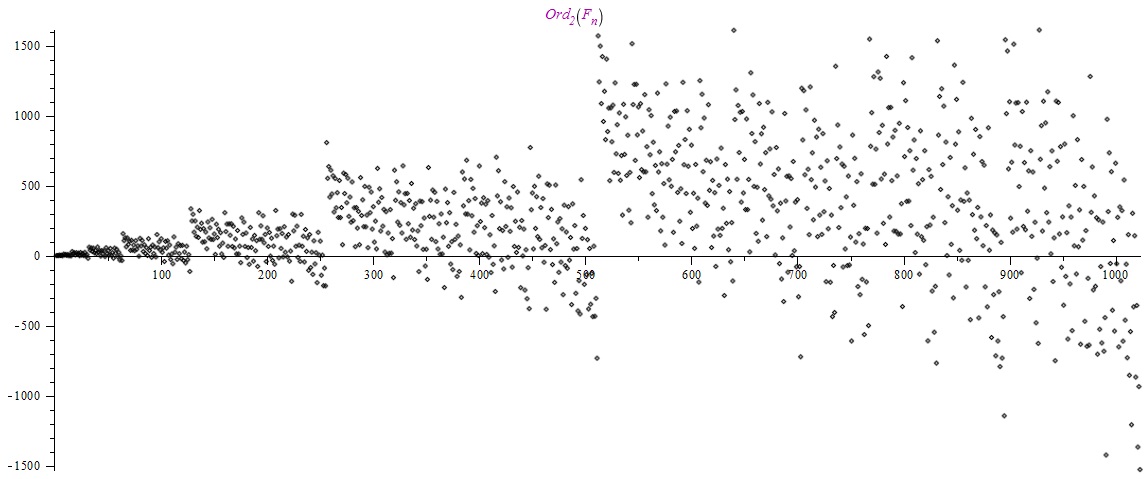
Figure 4.1. Values of ${\rm ord}_{2}(\overline{F}_{n})$, $1\leq n\leq 1023$.

We next consider the empirical distribution of the individual values of ${\rm ord}_{2}(\overline{F}_{n})$. Figure 4.2 plots a the rescaled values $\frac{1}{n}{\rm ord}_{2}(\overline{F}_{n})$ on the interval between $2^{k}\leq n<2^{k+1}$, ordered by size.

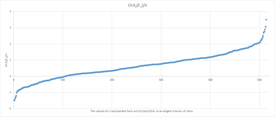
Figure 4.2. Sorted values of $\frac{1}{n}{\rm ord}_{2}(\overline{F}_{n})$, $512\leq n\leq 1024$.

This plot looks qualitatively similar to that for ${\rm ord}_{2}(\overline{G}_{n})$ in Figure 2.2, with the change that the median of the distribution is shifted downwards. The median of this empirical distribution is around $0.7$, suggesting that the average value of ${\rm ord}_{2}(\overline{F}_{n})$ is around $0.7n$ on this range $512\leq n\leq 1024$. In particular the median appears to be much smaller than $\frac{1}{2}n\log_{2}n$ for ${\rm ord}_{2}(\overline{G}_{n})$. The data is insufficient to guess at what rate the median of the distribution is growing: is it growing like $Cn$ or like $Cn\log_{2}n$?

Finally we study jumps of the function at $n=p^{r}-1$. Empirical data suggests that ${\rm ord}_{p}(F_{p^{r}-1})$ may be always non-positive, as shown for $p=2$ in Table 4.1 below. The last two columns suggest that these values seem to grow like a constant times $n\log_{2}n$. In Appendix A we present additional data for $p=3$, for $1\leq r\leq 10$, where we observe similar behavior occurs.

Power $r$	$N=2^{r}-1$	${\rm ord}_{2}(\overline{F}_{2^{r}-1})$	$-\frac{1}{N}{\rm ord}_{2}(F_{2^{r}-1})$	$-\frac{1}{N\log_{2}N}{\rm ord}_{2}(F_{2^{r}-1})$
$1$	$1$	$0$	$0.0000$	$0.0000$
$2$	$3$	$0$	$0.0000$	$0.0000$
$3$	$7$	$-1$	$0.1429$	$0.0509$
$4$	$15$	$-2$	$0.1333$	$0.0341$
$5$	$31$	$-19$	$0.6129$	$0.0586$
$6$	$63$	$-35$	$0.5555$	$0.0929$
$7$	$127$	$-113$	$0.8898$	$0.1273$
$8$	$255$	$-216$	$0.8471$	$0.1095$
$9$	$511$	$-733$	$1.4344$	$0.1594$
$10$	$1023$	$-1529$	$1.4946$	$0.1495$
$11$	$2047$	$-3830$	$1.8710$	$0.1701$
$12$	$4095$	$-7352$	$1.7953$	$0.1496$
$13$	$8191$	$-20348$	$2.4842$	$0.1910$
$14$	$16383$	$-41750$	$2.5484$	$0.1820$
$15$	$32767$	$-89956$	$2.7453$	$0.1830$

TABLE 4.1. Values at $N=2^{r}-1$ of ${\rm ord}_{2}(\overline{F}_{N})$.

4.3. Behavior of ${\rm ord}_{p}(\overline{F}_{n})$: hypothetical properties

The empirical data in Figures 4.1 and 4.2 together with Table 4.1 suggest that the following (unproved) hypothetical properties (P1)-(P4) might conceivably hold for all the functions $f_{p}(n):={\rm ord}_{p}(\overline{F}_{n})$ The first property concerns the sign of ${\rm ord}_{p}(\overline{F}_{n})$ at $n=p^{k}-1$.

Property (P1). For a given prime $p$ there holds

$$f_{p}({p^{k}-1})\leq 0\quad\mbox{ for all}\quad k\geq 1.$$

Furthermore $f_{p}(p^{k}-1)<0$ for all $k\geq 2$, with the exception $(p,k)=(2,2).$.

The second property concerns the sign of ${\rm ord}_{p}(\overline{F}_{n})$ at $n=p^{k}$.

Property (P2). For a given prime $p$ one has $f_{p}({p^{k}})>0$ for all all $k\geq 1$..

The third property concerns sign changes of ${\rm ord}_{p}(\overline{F}_{n})$.

Property (P3). For a given prime $p$ the inequalities $f_{p}(n)>0$ and $f_{p}(n)<0$ each occur infinitely often. Each may hold for a positive proportion of $n$, as $n\to\infty$.

The fourth property concerns the absolute magnitude of $|{\rm ord}_{p}(\overline{F}_{n})|$.

Property (P4). For a given prime $p$ there are are finite positive constants $C_{1,p},C_{2,p}$ such that, for all $n\geq 1$,

$$-C_{1,p}\,n\log_{p}n\leq f_{p}(n)\leq C_{2,p}\,n\log_{p}n.$$

We are far from establishing the validity of any of Properties (P1)-(P4) for $f_{p}(n)={\rm ord}_{p}(\overline{F}_{n})$. Because the fluctuations in Möbius function sums remain small for $n\leq 10000$, the computational evidence presented is a rather limited test of these properties. We are not completely convinced they are true. Perhaps Property (P1) holds for a given $p$ only for $k$ sufficiently large. In the next subsection we present limited theoretical evidence in their favor.

4.4. Evidence for hypothetical properties (P1)-(P4).

Properties (P1) and (P2) hold for the $k=1$ case of ${\rm ord}_{p}(\overline{F}_{n})$. We have verified computationally that Properties (P1), (P2) hold for all primes $p<1000$ when $k=2$. We have verified that Hypotheses (P1), (P2) hold for $p=2$ for exponents $1\leq k\leq 15$ and that for $p=3$ for exponents $1\leq k\leq 10$.

An interesting special case to consider is whether ${\rm ord}_{p}(\overline{F}_{p^{2}-1})<0$ holds for all $p\geq 3$. Note that this function of $p$ is complicated because it involves all values $\{\mu(k):1\leq k\leq p^{2}\}.$ To aid in its study, we give several formulas for this function.

Theorem 4.8.

Let $p\geq 3$ be prime.

(1) One has

$${\rm ord}_{p}(\overline{F}_{p^{2}-1})=\sum_{k=1}^{p-1}\mu(k)\,{\rm ord}_{p}(\overline{G}_{\lfloor\frac{p^{2}-1}{k}\rfloor})$$ (4.3)

(2) For $1\leq k\leq p-1$ write $\lfloor\frac{p^{2}-1}{k}\rfloor=a_{k}p+b_{k},~{}~{}~{}0\leq a_{k},b_{k}\leq p-1,$ then

$${\rm ord}_{p}(\overline{G}_{\lfloor\frac{p^{2}-1}{k}\rfloor})=a_{k}(p-1-b_{k}).$$ (4.4)

Here $a_{k}=\lfloor\frac{p-1}{k}\rfloor$ and $b_{k}=\lfloor\frac{p^{2}-1}{k}\rfloor-p\lfloor\frac{p-1}{k}\rfloor.$

(3) One has

$${\rm ord}_{p}(\overline{F}_{p^{2}-1})=(p-1)-\Big{(}\sum_{k=1}^{p-1}\mu(k)\lfloor\frac{p-1}{k}\rfloor b_{k}\Big{)}.$$ (4.5)

Remark 4.9.

In particular whenever $k|(p-1)$ one has $a_{k}=b_{k}=\frac{p-1}{k}$; these values include $k=1,2,\frac{p-1}{2},p-1$. One has ${\rm ord}_{p}(\overline{G}_{p^{2}-1})=0$ and ${\rm ord}_{p}(\overline{G}_{(p^{2}-1)/2})=\frac{(p-1)^{2}}{4},$ and the $k=2$ term makes a large negative contribution. This fact is sufficient to explain the negativity of ${\rm ord}_{p}(\overline{F}_{p^{2}-1})$ for small primes.

Proof.

(1) We have ${\rm ord}_{p}(\overline{G}_{n})=0$ for $1\leq n\leq p-1$, and $\lfloor\frac{p^{2}-1}{j}\rfloor\neq p$ for all integers $j$. The Möbius inversion formula (2.16) has all terms vanish for $\ell\geq p$, which yields (4.3).

(2) For $1\leq k\leq p-1$ we have

$$a_{k}=\lfloor\frac{p^{2}-1}{pk}\rfloor=\lfloor\frac{p-1}{k}\rfloor,$$

whence

$$b_{k}=\lfloor\frac{p^{2}-1}{k}\rfloor-p\lfloor\frac{p-1}{k}\rfloor$$

Using Theorem 2.3 we have

$${\rm ord}_{p}(\overline{G}_{n})=\frac{1}{p-1}(2{S}_{p}(n)-(n-1)d_{p}(n)).$$

Substituting $n=a_{k}p+b_{k}$ we find that

$$2{S}_{p}(n)=(a_{k}+b_{k})^{2}-(a_{k}+b_{k})+a_{k}(p-1)(a_{k}+p-1),$$

while

$$(n-1)d_{p}(n)=(a_{k}^{2}+a_{k}b_{k}-2a_{k})p+(b_{k}-1)(a_{k}+b_{k})+a_{k}.$$

A calculation yields (4.4).

(3) We have the identity, valid for all $n\geq 1$,

$$\sum_{k=1}^{n}\mu(k)\lfloor\frac{n}{k}\rfloor=1,$$ (4.6)

It is easily proved by induction on $n\geq 1$. Substituting the formula of (2) into that of (1) gives the result. ∎

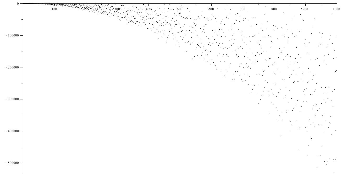
Figure 4.3. Values of ${\rm ord}_{p}(\overline{F}_{p^{2}-1})$ for prime $1\leq p\leq 1000$.

Figure 4.3 plots ${\rm ord}_{p}(F_{p^{2}-1})$ for $3\leq p\leq 1000$. The distribution of these values has a lower envelope which appears empirically to be of the form $-cN\log_{p}N$ with $c=0.25$, where $N=p^{2}-1.$ It has a pronounced scatter of points including some values rather close to $0$, but never crossing $0$. The observation suggests that there may be a barrier at $0$, and one may ask: Is there some arithmetic interpretation of the values ${\rm ord}_{p}(F_{p^{2}-1})$ that might justify their negativity, i.e. the truth of Property (P1) for $k=2$?

As an initial step in the direction of Property (P3), we show that ${\rm ord}_{p}(\overline{F}_{n})$ takes positive and negative values at least once, for each prime $p$.

Theorem 4.10.

For each prime $p$ the function ${\rm ord}_{p}(\overline{F}_{n})$ takes both positive and negative values.

1. For each $p\geq 2,$ ${\rm ord}_{p}(\overline{F}_{p})>0$ with ${\rm ord}_{p}(\overline{F}_{p})=p-1.$

2. For $p=2$, ${\rm ord}_{2}(\overline{F}_{7})=-1$. For odd primes $p$,

   $${\rm ord}_{p}(\overline{F}_{3p-1})=-(\frac{p-1}{2}),$$

   More generally, for $p\geq 3$,

   $${\rm ord}_{p}(\overline{F}_{n})<0\,\,\,\mbox{for}~{}~{}~{}\frac{8}{3}p\leq n\leq 3p-1.$$ (4.7)

Proof.

Write $F_{n}=\frac{N_{n}}{D_{n}}$ where $N_{n}$ is the product of the numerators of the positive Farey fractions $\frac{h}{k}$ of order $n$, and $D_{n}$ is the product of the denominators. (The quantities $N_{n}$ and $D_{n}$ will have a large common factor.) Now the reciprocal Farey product has

$${\rm ord}_{p}(\overline{F}_{n})={\rm ord}_{p}(D_{n})-{\rm ord}_{p}(N_{n}).$$

Choosing $n=p$, ${\rm ord}_{p}(N_{p})=0$ while ${\rm ord}_{p}(D_{p})=\varphi(p)=p-1$.

To find negative values, calculation gives ${\rm ord}_{2}(\overline{F}_{7})=-1$. Suppose now $p\geq 3$. For $2p\leq n\leq 3p-1$ we have ${\rm ord}_{p}(D_{n})=2(p-1)$, coming from the denominators $p$ and $2p$. For $p+1\leq n\leq 2p-1$ the Farey fraction $\frac{p}{n}$ contributes to ${\rm ord}_{p}(N_{m})$, for any $m\geq n$. For $2p+1\leq n\leq 3p-1$ the fraction $\frac{p}{n}$ similarly contributes one to ${\rm ord}_{p}(N_{m})$, as does $\frac{2p}{n}$ for odd values of $n$ in this interval. We conclude that for $2p+1\leq n\leq 3p-1$,

$${\rm ord}_{p}(N_{n})=(p-1)+\lfloor\frac{3}{2}(n-2p)\rfloor$$

This yields ${\rm ord}_{p}(N_{n})\geq 2p-1$ for $n\geq\frac{8}{3}p$, whence ${\rm ord}_{p}(\overline{F}_{n})<0$, giving (2). Finally, choosing $n=3p-1$ we obtain ${\rm ord}_{p}(\overline{F}_{3p-1})=-(\frac{p-1}{2}).$ ∎

In the direction of Property (P4), we have the weak bound

$$|{\rm ord}_{p}(\overline{F}_{n})|=O(n(\log n)^{2})$$

given in Theorem 4.6 above. We also have the Omega result

$${\rm ord}_{p}(\overline{F}_{n})=\Omega(n\log_{p}n),$$

because the individual jumps in the function ${\rm ord}_{p}(\overline{F}_{n})$ are at least as large as a constant times $n\log_{p}n$. Indeed, for $n=p^{k}$ we have

$${\rm ord}_{p}(\overline{F}_{p^{k}})-{\rm ord}_{p}(\overline{F}_{p^{k}-1})=k\varphi(p^{k})=kp^{k-1}(p-1)=(1-\frac{1}{p})n\log_{p}n.$$

This calculation implies that

$$\limsup_{n\to\infty}\frac{{\rm ord}_{p}(\overline{F}_{n})}{n\log_{p}n}-\liminf_{n\to\infty}\frac{{\rm ord}_{p}(\overline{F}_{n})}{n\log_{p}n}\geq 1-\frac{1}{p}.$$

Thus the assertion of Property (P4), if true, is qualitatively best possible.

4.5. When is the reciprocal Farey product $\overline{F}_{n}$ an integer?

This question was originally raised (and solved) in [3]. Their solution was obtained using (4.7) in Theorem 4.10, as follows.

Theorem 4.11.

Finitely many reciprocal Farey products $\overline{F}_{n}$ are integers. The largest such value is $n=58$.

Proof.

If $n$ has the property that there exists a prime $p$ satisfying

$$\frac{1}{3}(n+1)\leq p\leq\frac{3}{8}n,$$

then condition (4.7) of Theorem 4.10 will be satisfied and ${\rm ord}_{p}(\overline{F}_{n})<0$ certifies that $F_{n}$ is not an integer. The prime number theorem implies that for any $\epsilon>0$ and all sufficiently large $n$ the interval $(\frac{1}{3}n,\frac{3}{8}n]$ contains at least $\frac{1}{24}(1-\epsilon)\frac{n}{\log n}$ primes. In particular such a prime will exist for all sufficiently large $n$, whence there are only finitely many integer $\overline{F}_{n}$.

To obtain the numerical bound $n=58$ requires the use of prime counting estimates with explicit remainder terms, together with computer calculation for small $n$, described in the solution cited in [3]. ∎

4.6. Reciprocal Farey product $\overline{F}_{n}$ given in lowest terms

Now consider the reciprocal Farey product $\overline{F}_{n}$ as a rational fraction given in lowest terms, calling it $\overline{F}_{n}=\frac{\hat{D}_{n}}{\hat{N}_{n}}$, with

$$\hat{D}_{n}:=\frac{D_{n}}{(N_{n},D_{n})}\quad\mbox{and}\quad\hat{N}_{n}:=\frac{N_{n}}{(N_{n},D_{n})}.$$

We ask: What are the growth rates of $\hat{D}_{n}$ and $\hat{N}_{n}$?

We have no answer to this question and about it make the following remarks.

1. It is not clear whether $\log(\hat{N}_{n})$ and $\log(\hat{D}_{n})$ separately have smooth asymptotic behaviors as $n\to\infty$. However their difference does, since

   $$\log(\overline{F}_{n})=\log(\hat{D}_{n})-\log(\hat{N}_{n})=\frac{3}{\pi^{2}}n^{2}+O(n\log n),$$

   as follows using Theorem 3.19(1), (3.5) and the estimate $\psi(n)=O(n)$.

2. The function $\hat{N}_{n}$ initially grows much more slowly than $\hat{D}_{n}$. Theorem 4.11 gives $\hat{N}_{58}=1$, while $\hat{D}_{58}>10^{400}$. However Theorem 4.10(2) implies a nontrivial asymptotic lower bound for growth of $\log(\hat{N}_{n})$. It states that the product of all primes in the range $\frac{1}{3}n<p<\frac{3}{8}n$ divides $\hat{N}_{n}$, which since there are $\gg\frac{n}{\log n}$ prime numbers in this interval implies that there is a positive constant $c$ such that $\log(\hat{N}_{n})\gg n$ for all sufficiently large $n$.

3. We do not know what is the maximal order of growth of $\log(\hat{N}_{n})$. Properties (P3) and (P4), if true, allow the possibility that it could be close to the same order as the main term. That is, they suggest the possibility that there is a positive constant $c$ such that $\log(\hat{N}_{n})>cn^{2}$ infinitely often.

5. Farey product archimedean encoding of the Riemann hypothesis

We have already seen that results of Mikolás encode the Riemann hypothesis in terms of $\overline{F}_{n}$ via a formula

$${\nu}_{\infty}(\overline{F}_{n}):=\log(\overline{F}_{n})=\left(\Phi(n)-\frac{1}{2}\psi(n)\right)+R_{\overline{F}}(n),$$

which has the arithmetic main term $\Phi(n)-\frac{1}{2}\psi(n)$ on the right side, plus a remainder term $R_{\overline{F}}(n)$. The equivalence to the Riemann hypothesis is formulated as the remainder term bound $R_{\overline{F}}(n)=O(n^{1/2+\epsilon})$. The arithmetic main term has the feature that it has oscillations in lower-order terms of its asymptotics which are of size much bigger than the remainder term $R_{\overline{F}}(n)$; thus, this arithmetic main term is a complicated object, whose behavior is of interest in its own right.

In this section we will show that one can replace the arithmetic main term of Mikolás on the right side of his formula with a new arithmetic main term $\Phi_{\infty}(n)$ built entirely out of the quantities $\log(\overline{G}_{k})$ associated to unreduced Farey products $\overline{G}_{k}$. To do this we make use of the Möbius inversion formula in Theorem 2.5, and the splitting in (2.18) . The advantage of our reformulation is that with it one can define formal analogues for each finite prime $p$. On the left side, the quantity to approximate, $\log(\overline{F}_{n})$, has an analogue quantity defined for each prime, ${\rm ord}_{p}(\overline{F}_{n})$. On the right side, the new arithmetic main term $\Phi_{\infty}(n)$ we introduce has analogue quantities built out of replacing the quantities $\log(\overline{G}_{k})$ with ${\rm ord}_{p}(\overline{G}_{k})$ in suitable ways. This permits us to attempt reformulations of the Riemann hypothesis at each prime $p$ separately, as we describe in Section 6.

5.1. Farey product archimedean arithmetic main term

We introduce our new archimedean arithmetic term $\Phi_{\infty}(n)$ at the real place, and its associated remainder term $R_{\infty}(n)$ defined by

$$\overline{R}_{\infty}(n):=\log(\overline{F}_{n})-\Phi_{\infty}(n)$$ (5.1)

The archimedean arithmetic term $\Phi_{\infty}(n)$ is given by

$$\Phi_{\infty}(n):=\sum_{k=1+{K_{n}}}^{n}\mu(k)\Phi^{*}\Big{(}\left\lfloor\frac{n}{k}\right\rfloor\Big{)}+\sum_{k=1}^{{K_{n}}}\mu(k)\,\log(\overline{G}_{\lfloor n/k\rfloor}),$$ (5.2)

in which the function $\Phi^{*}(n)=n(n+1)/2$ counts the number of unreduced Farey products of order $n$, and we choose a cutoff $K_{n}\approx\sqrt{n}$. By collecting all terms with $\lfloor n/k\rfloor=\ell$ we may rewrite the archimedean arithmetic term above in the alternate form

$$\Phi_{\infty}(n)=\sum_{k=1}^{{K_{n}}}\mu(k)\,\log(\overline{G}_{\lfloor n/k\rfloor})+\sum_{\ell=1}^{{L_{n}}}\Big{(}M\left(\frac{n}{\ell}\right)-M\left(\frac{n}{\ell+1}\right)\Big{)}\frac{\ell(\ell+1)}{2},$$ (5.3)

in which ${L_{n}}\approx\sqrt{n}$ is determined by ${K_{n}}$, and vice versa. Using (2.16) and (2.18) we can express the remainder term $\overline{R}_{\infty}(n)$ as

$$\overline{R}_{\infty}(n)=\sum_{\ell=1}^{{L_{n}}}\left(M\left(\frac{n}{\ell}\right)-M\left(\frac{n}{\ell+1}\right)\right)\Big{(}\log(\overline{G}_{\ell})-\frac{\ell(\ell+1)}{2}\Big{)}.$$ (5.4)

For calculations reported below we chose

$${L_{n}}=\lfloor\sqrt{n}\rfloor=m,$$ (5.5)

in which case we have

$${K_{n}}=\begin{cases}\lfloor\sqrt{n}\rfloor-1&\quad\mbox{for}\quad m^{2}\leq n<m(m+1),\\ \lfloor\sqrt{n}\rfloor&\quad\mbox{for}\quad m(m+1)\leq n<(m+1)^{2}.\end{cases}$$ (5.6)

The definition (5.2) of the archimedean arithmetic term includes an initial sum that extends over the full range of summation $1\leq k\leq n$. This term is the contribution under Möbius inversion of the main term $\frac{1}{2}(\lfloor n/k\rfloor)(\lfloor n/k\rfloor+1)$ in the asymptotic formula for $\overline{G}_{\lfloor n/k\rfloor}$. The second sum in our archimedean main has the summation range from $1$ up to about $\sqrt{n}$. It is a “main term” obtained when using the Dirichlet hyperbola method for splitting sums

$$\sum_{k=1}^{n}F(\frac{n}{k})g(k)=\sum_{1\leq k\leq{K_{n}}}F(\frac{n}{k})g(k)+\sum_{{K_{n}}<k\leq n}F(\frac{n}{k})g(k).$$

into a “main term” and “remainder term”, compare [4, Lemma 2.1], [13, Sect. 3.4]. The two terms in the definition of $\Phi_{\infty}(n)$ account for the two parts of the Mikolás arithmetic main term, as explained below.

A justification for our definition of $\Phi_{\infty}(n)$ is the following result.

Theorem 5.1.

The Riemann hypothesis implies that for fixed $\epsilon>0$ as $n\to\infty$

$$\overline{R}_{\infty}(n)=O(n^{\frac{3}{4}+\epsilon}),$$ (5.7)

where the implied $O$-constant depends on $\epsilon$.

We defer the proof of Theorem 5.1 to Section 5.3. The proof shows that the initial sum on the right side of (5.2) is unconditionally of size $\Phi(x)+O(1)$ and shows that the second sum on the right side of (5.2) is, conditional on the Riemann Hypothesis, of size $-\frac{1}{2}\psi(x)+O(x^{\frac{3}{4}+\epsilon})$.

Based on Theorem 5.1 we propose:

Hypothesis $\overline{R}_{\infty}$. For each $\epsilon>0$ there holds, as $n\to\infty$,

$$\overline{R}_{\infty}(n)=O(n^{\frac{3}{4}+\epsilon}),$$ (5.8)

where the implied $O$-constant depends on $\epsilon$.

Theorem 5.1 seems weaker in appearance than the result of Mikolás in having a remainder term bounded by $O(x^{3/4+\epsilon})$ rather than $O(x^{1/2+\epsilon}),$ so it may seem that Hypothesis $\overline{R}_{\infty}$ might be weaker than the Riemann hypothesis. Subsequent work of the first author with R. C.Vaughan will show that the converse of Theorem 5.1 holds, and that Hypothesis $\overline{R}_{\infty}$ is actually equivalent to the Riemann hypothesis, In addition it will show the true magnitude of the error term is $\Omega(x^{\frac{3}{4}-\epsilon})$.

5.2. Remainder term $R_{\infty}(n)$: experimental data

Figure 5.1 presents empirical data on $\overline{R}_{\infty}(n)$. The function is bounded by $n^{3/4}$ over the given range, and its graph has a striking appearance exhibiting definite internal structure.

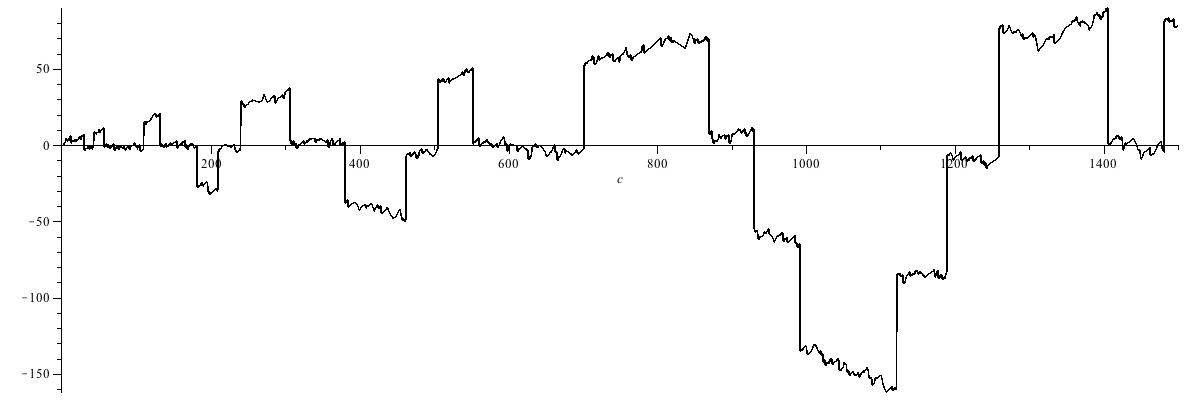
Figure 5.1. $\overline{R}_{\infty}(n)$, $1\leq n\leq 1500$.

The graph exhibits occasional large jumps of varying sign followed by slow variation of the function. It was noted by J. Arias de Reyna that the location of these jumps of the function visible in the graph in Theorem 5.1 are at a subset of the points $n=m(m+1)$. Subsequent work related these jumps to the hyperbola method splitting of the “main term” and “remainder term”. They occur only at values $m$ is squarefree, and the direction of each jump is that of $\mu(m)$.

5.3. Proof of Theorem 5.1

We partition the archimedean arithmetic term $\Phi_{\infty}(n)$ as

$$\Phi_{\infty}(n)=\Phi_{\infty,1}(n)+\Phi_{\infty,2}(n),$$

with initial sum $\Phi_{\infty,1}(n)$ defined by

$$\Phi_{\infty,1}(n)\,:=\quad\sum_{k=1}^{n}\mu(k)\Phi^{*}\Big{(}\left\lfloor\frac{n}{k}\right\rfloor\Big{)}=\frac{1}{2}\sum_{k=1}^{n}\mu(k)\left\lfloor\frac{n}{k}\right\rfloor\Big{(}\left\lfloor\frac{n}{k}\right\rfloor+1\Big{)}$$ (5.9)

and the second sum $\Phi_{\infty,2}(n)$ defined by

$$\Phi_{\infty,2}(n)\,:=\quad\sum_{k=1}^{{K_{n}}}\mu(k)\,\Big{(}\log(\overline{G}_{\lfloor n/k\rfloor})-\Phi^{*}\Big{(}\left\lfloor\frac{n}{k}\right\rfloor\Big{)}\Big{)},\quad\quad$$ (5.10)

with ${K_{n}}$ given by (5.6). We first derive an unconditional formula for the initial sum $\Phi_{\infty,1}(n)$.

Theorem 5.2.

Set $\Phi(n)=\sum_{k=1}^{n}\varphi(k)$. Then one has

$$\Phi(n)=\frac{1}{2}\sum_{k=1}^{n}\mu(k)\lfloor\frac{n}{k}\rfloor(\lfloor\frac{n}{k}\rfloor+1),$$ (5.11)

so that $\Phi(n)=\Phi_{\infty,1}(n)$.

Proof.

We first show that

$$\Phi(n)=\frac{1}{2}\Big{(}\sum_{k=1}^{n}\mu(k)(\lfloor\frac{n}{k}\rfloor)^{2}\Big{)}+\frac{1}{2}.$$ (5.12)

This equality is proved by induction on $n$; call its right side $S(n)$. The extra term $\frac{1}{2}$ on the right side is needed to establish the base case $n=1$. For the induction step, suppose $S(n)=\Phi(n)$ for a given $n$. Since $\lfloor\frac{n+1}{k}\rfloor=\lfloor\frac{n}{k}\rfloor$ unless $k\mid(n+1)$, we have

$$S(n+1)-S(n) = \frac{1}{2}\sum_{d|(n+1)}\mu(d)\Big{(}\lfloor\frac{n+1}{d}\rfloor^{2}-\lfloor\frac{n}{d}\rfloor^{2}\Big{)}$$

$$= \frac{1}{2}\sum_{d|(n+1)}\mu(d)\Big{(}2(\frac{n+1}{d})-1\Big{)}$$

$$= \sum_{d|(n+1)}\mu(d)\frac{n+1}{d}-\frac{1}{2}\left(\sum_{d|(n+1)}\mu(d)\right).$$

$$= \varphi(n+1),$$

This shows $S(n+1)=\Phi(n+1),$ completing the induction step, proving (5.12).

To establish (5.11), comparing the definition (5.9) of $\Phi_{\infty,1}(n)$ with the right side of (5.12), we obtain,

$$\Phi_{\infty,1}(n)=\Phi(n)-\frac{1}{2}+\frac{1}{2}\sum_{k=1}^{n}\mu(k)\lfloor\frac{n}{k}\rfloor=\Phi(n)$$

where the last equality used (4.6). ∎

Remark 5.3.

Combining (5.12) with the known asymptotic for $\Phi(n)$ yields

$$\frac{1}{2}\sum_{k=1}^{n}\mu(k)(\lfloor\frac{n}{k}\rfloor)^{2}=\frac{3}{\pi^{2}}n^{2}+O(n\log n).$$

Here the remainder term $E(n)=\Phi(n)-\frac{3}{\pi^{2}}n^{2}$ is known to have large oscillations of magnitude at least $\Omega(n\sqrt{\log\log n})$ (see Section 3.2). One can consider a similar sum which does not apply the fractional part function, and obtain a similar unconditional estimate

$$\frac{1}{2}\Big{(}\sum_{k=1}^{n}\mu(k)(\frac{n}{k})^{2}\Big{)}=\frac{3}{\pi^{2}}n^{2}+O(n).$$ (5.13)

Under the assumption of the Riemann hypothesis, one can establish a much smaller error term

$$\frac{1}{2}\Big{(}\sum_{k=1}^{n}\mu(k)(\frac{n}{k})^{2}\Big{)}=\frac{3}{\pi^{2}}n^{2}+O(n^{\frac{1}{2}+\epsilon}).$$

Comparing the right side of (5.12) with (5.13) reveals that the oscillations in the remainder term $E(n)$ are coming from the application of the floor function in the sum (5.12).

We next derive estimates for $\Phi_{\infty,2}(n)$.

Theorem 5.4.

(1) There holds unconditionally

$$\Phi_{\infty,2}(n)=\frac{n}{2}\sum_{1\leq k\leq\sqrt{n}}\frac{\mu(k)}{k}\log k-\frac{n}{2}\log\left(\frac{2\pi n}{e}\right)\sum_{1\leq k\leq\sqrt{n}}\frac{\mu(k)}{k}+O\left(\sqrt{n}\log n\right).$$ (5.14)

(2) Assuming the Riemann hypothesis, for each $\epsilon>0$ there holds

$$\Phi_{\infty,2}(n)=-\frac{1}{2}\psi(n)+O\big{(}n^{3/4+\epsilon}\big{)}.$$ (5.15)

where $\psi(x):=\sum_{n\leq x}\Lambda(n)$.

Proof.

(1) To prove (1) from Theorem 2.1 we have

$$\log(\overline{G}_{\lfloor n/k\rfloor})=\Phi^{\ast}\left(\left\lfloor\frac{n}{k}\right\rfloor\right)-\frac{1}{2}\left\lfloor\frac{n}{k}\right\rfloor\log\left(\left\lfloor\frac{n}{k}\right\rfloor\right)+\Big{(}\frac{1}{2}-\log(\sqrt{2\pi})\Big{)}\left\lfloor\frac{n}{k}\right\rfloor+O\Big{(}\log\Big{(}\left\lfloor\frac{n}{k}\right\rfloor\Big{)}\Big{)}.$$

We write $\lfloor n/k\rfloor=n/k-\{n/k\}$ and obtain that

$$\log(\overline{G}_{\lfloor n/k\rfloor})-\Phi^{\ast}\left(\left\lfloor\frac{n}{k}\right\rfloor\right)$$

can be written as

$$-\frac{1}{2}\left(\frac{n}{k}-\Big{\{}\frac{n}{k}\Big{\}}\right)\left(\log\frac{n}{k}+\log\left(1-\frac{k}{n}\Big{\{}\frac{n}{k}\Big{\}}\right)+2\log\left(\frac{2\pi}{e}\right)\right)+O\left(\log\left(\frac{n}{k}\right)\right).$$

Using the estimate $\log(1-\frac{k}{n}\{\frac{n}{k}\})=O(\frac{k}{n})$ valid for $1\leq k\leq\lfloor\sqrt{n}\rfloor$, and noting that in all cases $\lfloor\sqrt{n}\rfloor-1\leq{K_{n}}\leq\lfloor\sqrt{n}\rfloor$, we obtain unconditionally

$$\Phi_{\infty,2}(n)=-\frac{n}{2}\sum_{1\leq k\leq\sqrt{n}}\frac{\mu(k)}{k}\log\frac{n}{k}-\log\left(\sqrt{\frac{2\pi}{e}}\right)\sum_{1\leq k\leq\sqrt{n}}\mu(k)\,\frac{n}{k}+O\Big{(}\sqrt{n}\log n\Big{)}.$$ (5.16)

Using $\log\frac{n}{k}=\log n-\log k$ in the first term, simplifying and collecting terms yields (5.14).

(2) To prove (2), first, assuming the Riemann hypothesis, we have the estimate

$$\sum_{1\leq k\leq\sqrt{n}}\frac{\mu(k)}{k}=O(n^{-1/4+\epsilon}).$$ (5.17)

To show this, we start from the conditionally convergent sum

$$\sum_{k=1}^{\infty}\frac{\mu(k)}{k}=0,$$

a statement known to be equivalent to the Prime Number Theorem. We then have

$$\sum_{k=1}^{N}\frac{\mu(k)}{k}=-\sum_{k=N+1}^{\infty}\frac{\mu(k)}{k}.$$

By partial summation, assuming RH, we obtain

$$\sum_{k=N+1}^{\infty}\frac{\mu(k)}{k} = \sum_{k=N+1}^{\infty}(M(k)-M(k-1))\frac{1}{k}$$

$$= \frac{M(N)}{N+1}+\sum_{k=N+1}^{\infty}M(k)\big{(}\frac{1}{k}-\frac{1}{k+1}\big{)}$$

$$= O\Big{(}N^{-1/2+\epsilon}+\sum_{k=N+1}^{\infty}\frac{\,k^{1/2+\epsilon}}{k(k+1)}\Big{)}=O\Big{(}N^{-1/2+\epsilon}\Big{)}.$$

Choosing $N=\sqrt{n}$ yields (5.17).

Second, assuming the Riemann hypothesis, we have the estimate

$$\sum_{1\leq k\leq\sqrt{n}}\frac{\mu(k)}{k}\log k=-1+O(n^{-\frac{1}{4}+\epsilon}\log n).$$ (5.18)

To show that, we start from the conditionally convergent sum

$$\sum_{k=1}^{\infty}\frac{\mu(k)}{k}\log k=\frac{d}{ds}(\frac{1}{\zeta(s)})|_{s=1}=-1,$$

again a result at the depth of the Prime Number Theorem. The result (5.18) is proved by a similar partial summation argument to the above.

The estimate (5.17) allows us to bound the second sum on the right in (5.14) by $O(n^{3/4+\epsilon})$. The estimate (5.18) allows us to estimate the first sum on the right in (5.14) by $-\frac{1}{2}n+O(n^{3/4+\epsilon})$. In consequence, the RH yields

$$\Phi_{\infty,2}(n)=-\frac{1}{2}n+O(n^{3/4+\epsilon}).$$

Third, the Riemann hypothesis is well known to be equivalent to the assertion

$$\psi(n)=n+O\Big{(}n^{1/2}(\log n)^{2}\Big{)}.$$

This fact proves (2). ∎

Proof of Theorem 5.1..

We assume that the Riemann hypothesis holds. On combining Theorem 5.2 with Theorem 5.4 (2), we obtain

$$\Phi_{\infty}(n)=\Phi_{\infty,1}(n)+\Phi_{\infty,2}(n)=\Phi(n)-\frac{1}{2}\psi(n)+O(n^{\frac{3}{4}+\epsilon}).$$

Combining this estimate with Mikolas’s Theorem 3.1 gives the estimate

$$\log(\overline{F}_{n})=\Phi_{\infty}(n)+O(n^{3/4+\epsilon}),$$

as desired. ∎

6. Is there an ${\rm ord}_{p}(\overline{F}_{n})$ analogue of the Riemann hypothesis?

The problem of determining the behavior of the functions ${\rm ord}_{p}(\overline{F}_{n})$ for a fixed prime $p$ may be a difficult one, because the analogous problem at the real place encodes the Riemann hypothesis, in the form Theorem 3.1 (2). One may ask more: Is it possible to encode the Riemann hypothesis itself at a single prime $p$, in terms of the behavior of ${\nu}_{p}(\overline{F}_{n})={\rm ord}_{p}(\overline{F}_{n})$ as $n\to\infty$?

In Section 5 we reformulated the Riemann hypothesis entirely in terms of the sizes $\log(\overline{F}_{n})$ and $\log(\overline{G}_{n})$ of Farey products and unreduced Farey products, respectively. The advantage of this reformulation is that has formal analogues defined for each finite prime $p$. On the left side, the quantity to approximate, $\log(\overline{F}_{n})$, has an analogue quantity defined for each prime, ${\rm ord}_{p}(\overline{F}_{n})$. On the right side, the new arithmetic main term $\Phi_{\infty}(n)$ we introduced has analogue quantities built out of replacing the quantities $\log(\overline{G}_{k})$ with ${\rm ord}_{p}(\overline{G}_{k})$ in suitable ways.

The new arithmetic main terms that we introduce this way are necessarily arithmetic functions exhibiting oscillations, because ${\rm ord}_{p}(\overline{F}_{n})$ exhibits oscillations and sign changes. These terms contain new kinds of arithmetic information which may be of interest in their own right, encoded as new sorts of arithmetic sums mixing the Möbius function with base $p$ radix expansion data. We will see there is more than one possible choice to consider for these “main terms” for a finite prime $p$. With each choice we have an associated remainder term, and we study these remainder terms experimentally.

In parallel with the archimedean case we expect the Riemann hypothesis to manifest itself in bounds on the size of remainder terms. We present below computational results that suggest such a formulation may be possible.

6.1. Arithmetic main terms and remainder terms for finite primes $p$

We now formulate “arithmetic main terms” for ${\rm ord}_{p}(\overline{F}_{n})$. For each prime $p$ we can define by analogy a decomposition

$${\nu}_{p}(\overline{F}_{n})=\Phi_{p}(n)+\overline{R}_{p}(n).$$ (6.1)

by making a suitable choice of a $p$-adic arithmetic term. It is not clear a priori whether there should be included an analogue of the first term on the right side of (5.2) or not. We therefore experimentally investigate three plausible choices for the arithmetic term, denoting them $\Phi_{p,j}(n)$ for $0\leq j\leq 2$, in which we may or may not choose to include a correction term of quantities summed over the whole interval $1\leq k\leq n$. We recall the formula

$${\rm ord}_{p}(\overline{G}_{n})=\frac{2}{p+1}S_{p}(n)-\frac{n-1}{p+1}d_{p}(n)$$

given in Theorem 2.3, which splits ${\rm ord}_{p}(\overline{G}_{n})$ into a smooth term and an oscillatory term, respectively. We consider the options whether to remove none or one of the two sums on the right side over the whole interval $1\leq k\leq n$.

The three options are first, to have no correction term,

$$\Phi_{p,0}(n):=\sum_{k=1}^{{K_{n}}}{}\mu(k)\,\Big{(}{\rm ord}_{p}(\overline{G}_{\lfloor n/k\rfloor})\Big{)},$$ (6.2)

or second, to add a correction term that removes the contribution of the $d_{p}(n)$,

$$\Phi_{p,1}(n):=\Phi_{p,0}(n)-\frac{n-1}{p-1}\left(\sum_{k=1+{K_{n}}}^{n}\mu(k)d_{p}\left(\Big{\lfloor}\frac{n}{k}\Big{\rfloor}\right)\right),$$ (6.3)

or third, to have a correction term that removes the contribution of the $S_{p}(n)$,

$$\Phi_{p,2}(n):=\Phi_{p,0}(n)-\frac{2}{p-1}\Big{(}\sum_{k={K_{n}}+1}^{n}\mu(k)S_{p}(\lfloor\frac{n}{k}\rfloor)\Big{)}.$$ (6.4)

In each case the remainder term $\overline{R}_{p,j}(n)$ is defined by (6.1) for $j=0,1,2$ with the $K_{n}$ is as defined in (5.6). The remainder terms $\overline{R}_{p,j}(n)$in the three cases are explicitly given by

$$\overline{R}_{p,0}(n)\quad=\quad\sum_{\ell=1}^{{L_{n}}}\Big{(}M\left(\frac{n}{\ell}\right)-M(n/(\ell+1)\Big{)}\,\big{(}{\rm ord}_{p}(G_{\ell})\big{)},\quad\quad\quad\quad$$

$$\overline{R}_{p,1}(n) = \sum_{\ell=1}^{{L_{n}}}\Big{(}M\left(\frac{n}{\ell}\right)-M\Big{(}\frac{n}{\ell+1}\Big{)}\Big{)}\,\big{(}{\rm ord}_{p}(G_{\ell})+\frac{\ell-1}{p-1}d_{p}(\ell)\big{)}$$

$$= \sum_{\ell=1}^{{L_{n}}}\Big{(}M\left(\frac{n}{\ell}\right)-M\Big{(}\frac{n}{\ell+1}\Big{)}\Big{)}\,\Big{(}\frac{2}{p-1}S_{p}(\ell)\Big{)},$$

$$\overline{R}_{p,2}(n) = \sum_{\ell=1}^{{L_{n}}}\Big{(}M\left(\frac{n}{\ell}\right)-M\Big{(}\frac{n}{\ell+1}\Big{)}\Big{)}\,\big{(}{\rm ord}_{p}(G_{\ell})-\frac{2}{p-1}S_{p}(\ell)\big{)}$$

$$= -\sum_{\ell=1}^{{L_{n}}}\Big{(}M\left(\frac{n}{\ell}\right)-M\Big{(}\frac{n}{\ell+1}\Big{)}\,\Big{(}\frac{\ell-1}{p-1}d_{p}(\ell)\Big{)}.$$

With these definitions we have the identity

$$\overline{R}_{p,0}(n)=\overline{R}_{p,1}(n)+\overline{R}_{p,2}(n).$$ (6.5)

For our calculations we choose ${L_{n}}=\lfloor\sqrt{n}\rfloor$ as above.

The formulas for $\Phi_{p,j}(n)$ embody arithmetic sums of new types, which involve Möbius function values multiplied against base $p$ radix expansion data of $k$ with $1\leq k\leq n$.

6.2. Remainder terms for $p=3$: experimental data

The following figures give data for $p=3$ for these three choices of remainder terms $\overline{R}_{p,j}(n).$

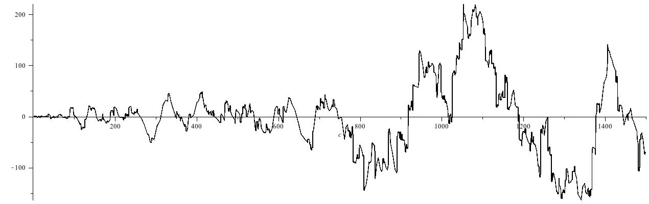
Figure 6.1. $\overline{R}_{3,0}(n)$, $1\leq n\leq 1500$.

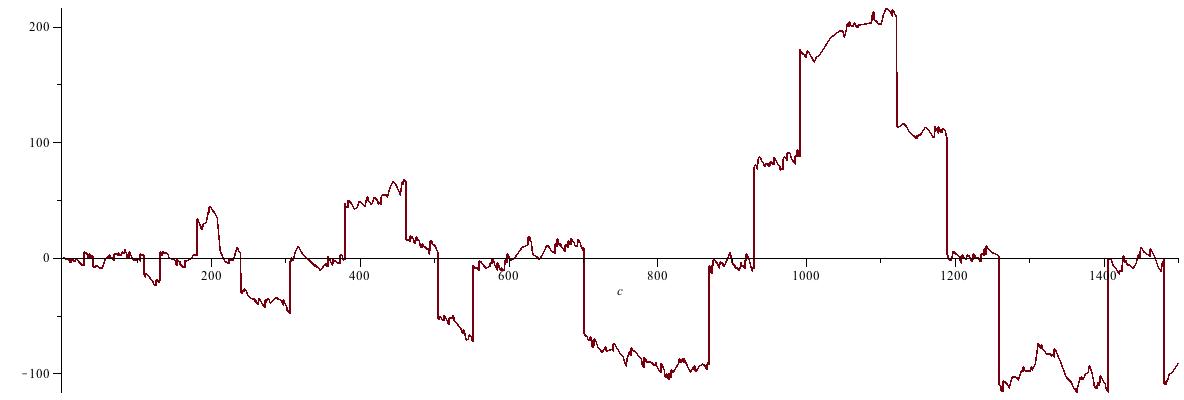
Figure 6.2. $\overline{R}_{3,1}(n)$, $1\leq n\leq 1500$.

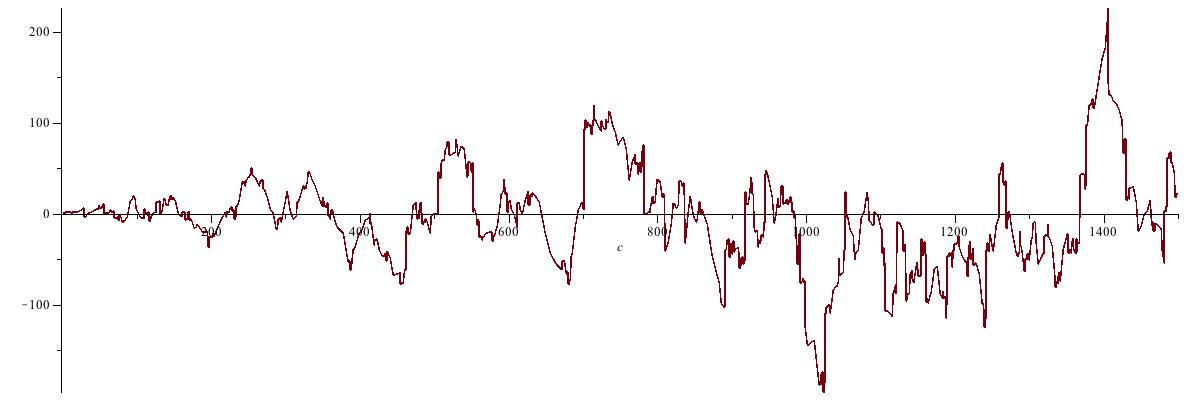
Figure 6.3. $\overline{R}_{3,2}(n)$, $1\leq n\leq 1500$.

In these plots all three remainder terms seem roughly the same size; this size however is slightly larger in magnitude than that seen for $\overline{R}_{\infty}(n)$. The identity (6.5) implies that either all three sums are of the same order of magnitude, or else one sum is significantly smaller than the other two.

We observe the surprising feature that the graph of $\overline{R}_{3,1}(n)$ in Figure 6.2 (more precisely of its negative $-\overline{R}_{3,1}(n)$) has a striking qualitative resemblance to the remainder term $\overline{R}_{\infty}(n)$. It has large abrupt jumps and some relatively flat spots, with jumps at exactly the same points as for $\overline{R}_{\infty}(n)$; the jumps appear to be larger than that of $R_{\infty}(n)$ by a factor of roughly $\frac{5}{3}$. We found that similar qualitative behavior occurs for $-\overline{R}_{2}(n)$ and $-\overline{R}_{5}(n)$ over the same range, with identical jump locations and multiplicative scaling factors of jump sizes roughly $3$ and $\frac{5}{4}$, respectively.

6.3. Remainder term growth rates: hypotheses

On the strength of the empirical observations above , we formulate for consideration the following hypotheses.

Hypothesis $\overline{R}_{p,1}$. For each fixed $\epsilon>0$ there holds, as $n\to\infty$,

$$\overline{R}_{p,1}(n)=O(n^{\frac{3}{4}+\epsilon}).$$ (6.6)

The similarity of the shape and magnitude of the plot of the remainder term $\overline{R}_{3,1}(n)$ to that of $\overline{R}_{\infty}(n)$, including the jump sizes, is striking. The structure and location of the jumps is explainable as an artifact the hyperbola method; the jumps are at $n=m(m+1)$ with $m$ squarefree and the jump directions are $-\mu(m)$. The hypothesis above concerns the growth rate of the reminder term and not its appearance, and one may ask whether this growth rate might be related to the Riemann hypothesis.

Since the plots of all three of the $\overline{R}_{3,j}(n)$ above empirically appear to be about the same size, we also propose for consideration:

Hypothesis $\overline{R}_{p,2}$. For each fixed $\epsilon>0$ there holds, as $n\to\infty$,

$$\overline{R}_{p,2}(n)=O(n^{\frac{3}{4}+\epsilon}).$$ (6.7)

We have no theoretical evidence supporting Hypothesis $\overline{R}_{p,2}$, but we have checked it empirically for other small primes, on limited data sets. We speculate that Hypothesis $\overline{R}_{p,2}$, if true, might encode arithmetic data specific to the prime $p$, directly relating the Möbius function and the base $p$ expansions of integers, not necessarily related to the Riemann hypothesis.

Besides Hypothesis $\overline{R}_{p,1}$ and $\overline{R}_{p,2}$, one may formulate in parallel a third hypothesis.

Hypothesis $\overline{R}_{p,0}$, For each fixed $\epsilon>0$ there holds, as $n\to\infty$,

$$\overline{R}_{p,0}(n)=O(n^{\frac{3}{4}+\epsilon}).$$ (6.8)

The additive identity (6.5) relating the $\overline{R}_{p,j}$ for $0\leq j\leq 2$ above shows that the truth of any two of these hypotheses would imply the truth of the third. We have no independent theoretical evidence supporting Hypothesis $R_{p,0}$.

7. Concluding Remarks: Arithmetic encodings of the Riemann hypothesis

To summarize our experimental work in Section 5 and 6 , we have found:

1. The remainder term $\overline{R}_{\infty}(n)$ plotted in Figure 5.1 is provably related to the Riemann hypothesis (via Theorem 5.1) and its plots reveal a striking internal structure of jumps worthy of further investigation.

2. The plot for $p=3$ of $\overline{R}_{3,1}(n)$ pictured in Figure 6.2 exhibits a similar internal structure to $\overline{R}_{\infty}(n)$, which implies nearly perfect correlation of the statistic $\overline{R}_{3,1}(n)$ with $\overline{R}_{\infty}(n).$ Similar internal structure was found in plots for $p=2$ and $p=5$ (not pictured).

The observation (2) was surprising, in that the quantities defining the statistic $\overline{R}_{p,1}(n)$ seemed very different from those defining $\overline{R}_{\infty}(n)$. Subsequent investigation revealed that the main features in these plots, with their pattern of large jumps followed by slow variation, can be explained as being an artifact of the “hyperbola method” truncation. The jumps are located at points $n=m(m+1)$ where $m$ is squarefree, and the sign of the jumps is related to $\mu(m)$. This direct connection of the error term with the Möbius function indicates that the zeta zeros influence at least part of its behavior. The Riemann hypothesis may possibly be encoded in the growth rates of the remainder terms; this topic is left for further investigation. Our data are insufficient to give a reliable guess on this growth rate. The data obtained is at least consistent with the possibility that the Riemann hypothesis may be directly visible in the growth rate of the remainder term statistics of ${\rm ord}_{p}(F_{n})$ at a fixed finite prime $p$. Larger scale computations are needed to confirm or disconfirm the possible $O(n^{\frac{3}{4}+\epsilon})$ behavior of this remainder term.

Acknowledgments

We thank J. Arias de Reyna, R. C. Vaughan and the two reviewers for helpful comments on this paper. The first author thanks Harm Derksen for bringing up questions on Farey products, resulting in [2], [3]. Work of H. Mehta on this project started as part of an REU program at the University of Michigan, with the first author as mentor.

Appendix A: Empirical Results for $p=3$

This Appendix presents plots and tables for ${\rm ord}_{p}(\overline{F}_{n})$ for $p=3$, supplementing the data for $p=2$ given in graphs and tables in Section 4.3.

Figure A.1 plots the values of ${\rm ord}_{4}(\overline{F}_{n})$ for $1\leq n<1214$. The cutoff value for this table is not a power of $3$, since $3^{6}=729$ and $3^{7}=2187$. It was chosen to be roughly $1/23^{7}$, the same size as the cutoff value for powers of $2$ for the graph in Section 4.3.

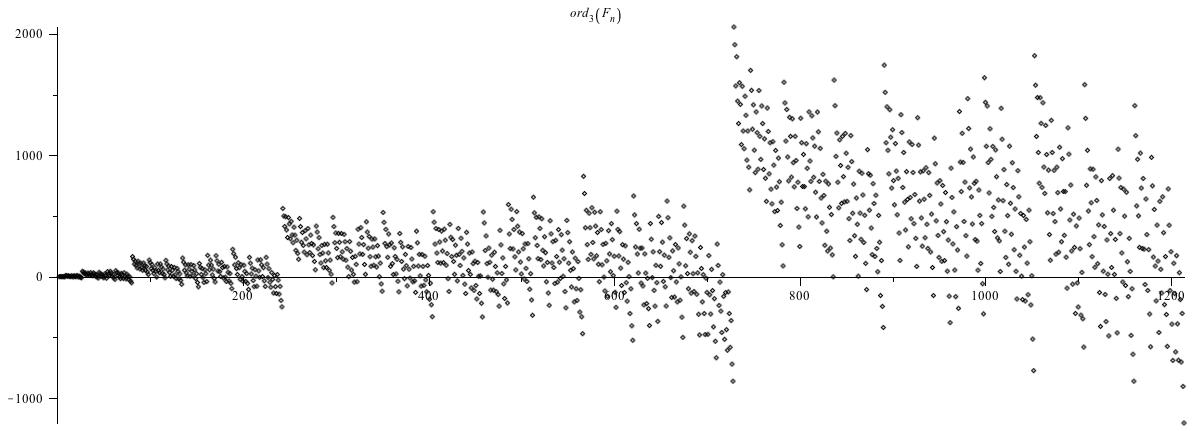
Figure A.1. ${\rm ord}_{3}(\overline{F}_{n})$, $1\leq n\leq 1214$.

Table A.1 presents data on the jump for ${\rm ord}_{p}(\overline{F}_{p^{k}-1})$ to ${\rm ord}_{p}(\overline{F}_{p^{k}})$ for the prime $p=3$. This data may be compared with Table 4.1 for $p=2$.

Power $r$	$N=3^{r}-1$	${\rm ord}_{3}(\overline{F}_{3^{r}-1})$	$-\frac{1}{N}{\rm ord}_{3}(F_{3^{r}-1})$	$-\frac{1}{N\log_{3}N}{\rm ord}_{3}(F_{3^{r}-1})$
$1$	$2$	$0$	$0.0000$	$0.0000$
$2$	$8$	$-1$	$0.1250$	$0.0538$
$3$	$26$	$-9$	$0.3461$	$0.1167$
$4$	$80$	$-50$	$0.6250$	$0.1567$
$5$	$242$	$-248$	$1.0248$	$0.2051$
$6$	$728$	$-860$	$1.1813$	$0.1969$
$7$	$2186$	$-3333$	$1.5247$	$0.2178$
$8$	$6560$	$-12380$	$1.8872$	$0.2359$
$9$	$19682$	$-45773$	$2.3256$	$0.2584$
$10$	$59048$	$-148338$	$2.5122$	$0.2512$

TABLE A.1. Values at $N=3^{r}-1$ of ${\rm ord}_{3}(\overline{F}_{N})$.

References

- [1] H. Delange, Sur la fonction sommatoire de la fonction Somme des chiffres . L’Enseign. Math. 21 (1975), no. 1, 31–47.
- [2] H. Derksen and J. C. Lagarias, Problem 11594. An Integral Product. Amer. Math. Monthly 118 (2011), no. 8, 747. [Solution 120 (2013), 856–857.]
- [3] H. Derksen and J. C. Lagarias, Problem 11601. The product of Farey series. Amer. Math. Monthly 118 (2011), no. 9, 846. [Solution 120 (2013), 857–858.]
- [4] H. Diamond, Elementary methods in the study of the distribution of prime numbers, Bull. Amer. Math. Soc., N. S. 7 1982), no. 3, 553–589.
- [5] J. Franel, Les suites de Farey et les problèmes des nombres premiers. Nachr. Ges. Wiss. Göttingen. Math-Phys,. Kl. 1924 (1924), 198–201.
- [6] A. Granville, Arithmetic properties of binomial coefficients. I. Binomial coefficients modulo prime powers. Organic mathematics (Burnaby, BC, 1995), 253–276, CMS Conf. Proc. 20, Amer. Math. Soc. : Providence, RI 1997.
- [7] G. H. Hardy, and E. M. Wright, An Introduction to the Theory of Numbers (Fifth Edition). Oxford University Press: Oxford 1979.
- [8] M. N. Huxley, The Distribution of Prime Numbers. Large sieves and zero-density theorems. Oxford Univ. Press: Oxford 1972.
- [9] J. Kaczorowski and K. Wiertelak, Smoothing arithmetic error terms: the case of the Euler -function, Math. Nachr. 283 (2010), no. 11, 1637–1645.
- [10] J. Kaczorowski and K. Wiertelak, Oscillations of the remainder term associated to the Euler totient function, J. Number Theory 130 (2010), 2683–2700.
- [11] S. Kanemitsu and M. Yoshimoto, Farey series and the Riemann hypothesis. Acta Arithmetica 75 (1996), No. 4, 351–374.
- [12] S. Kanemitsu and M. Yoshimoto, Euler products, Farey series and the Riemann hypothesis. Publ. Math. Debrecen 56 (2000), no. 3-4, 431–449.
- [13] J. C. Lagarias, Euler’s constant: Euler’s work and modern developments. Bull. Amer. Math. Soc. (N. S.) 50 (2013), no. 4, 527–628.
-
[14]
J. C. Lagarias and H. Mehta,
Products of binomial coefficients and unreduced Farey fractions,
International J. Number Theory, 12:1 (2016), 57?91
DOI:10.1142/S1793042116500044 eprint: arXiv:1409.4145 - [15] E. Landau, Bemerkungen zu der vorshehenden Abhandlung von Herrn Franel, Nachr. Ges. Wiss. Göttingen, Math-Phys,. Kl. 1924 (1924), 202–206.
- [16] E. Landau, Vorlesungen über Zahlentheorie. Teil II. Teubner: Leipzig 1927. (Reprint: Chelsea).
- [17] F. Mertens, Ueber einige asymptotische Gesetze der Zahlentheorie, J. reine angew. Math. 77 (1874), 289–338.
- [18] M. Mikolás, Farey series and their connection with the prime number problem I. Acta Sci. Math. (Szeged) 13 (1949), 93–117.
- [19] M. Mikolás, Farey series and their connection with the prime number problem II. Acta Sci. Math. (Szeged) 14 (1951), 5–21.
- [20] H. L. Montgomery, Fluctuations in the mean of Euler’s phi function. Proc. Indian Acad. Sci. (Math. Sci.) 97 (1987), no. 1–3, 239–245.
- [21] G. Tenenbaum, Introduction to Analytic and Probabilistic Number Theory, Cambridge Univ. Press: Cambridge 1995.
- [22] G. Tenenbaum, Sur la non-dérivabilité de fonctions périodiques associaiées à certaines formules sommatoires. In: The Mathematics of Paul Erdős, I. Berlin: Springer-Verlag 1997, pp. 117–128.
- [23] E. C. Titchmarsh, The Theory of the Riemann Zeta Function, Second Edition. Revised by D. R. Heath-Brown. Oxford U. Press: Oxford 1986.
- [24] A. Walfisz, Weylsche exponentialsummen in der neuren Zahlentheorie. VEB Deutscher Verlag Wiss. No. 16. Altenberg, GDR 1962.