The discontinuity of the specific heat for the 5D Ising model

Abstract

In this paper we investigate the behaviour of the specific heat around the critical point of the Ising model in dimension 5 to 7. We find a specific heat discontinuity, like that for the mean field Ising model, and provide estimates for the left and right hand limits of the specific heat at the critical point. We also estimate the singular exponents, describing how the specific heat approaches those limits. Additionally, we make a smaller scale investigation of the same properties in dimension 6 and 7, and provide strongly improved estimates for the critical termperature $K_{c}$ in $d=5,6,7$ which bring the best MC-estimate closer to those obtained by long high temperature series expanions.

I Introduction

The Ising model in dimension $d=5$, being strictly larger than the upper critical dimension $d_{c}=4$ of the model, has been studied by many authors, and has been the focus of a long running debate regarding its finite size scaling behaviour. We refer the reader to Lundow and Markström (2014) for a discussion of that topic. However, even regarding the infinite size limit of the model there are still interesting open questions. For $d>d_{c}$ it is rigorously known that on the $d$-dimensional hypercubic lattice the critical exponents of model takes their mean field values. This was first proven in Sokal (1979); Aizenman (1981, 1982); Aizenman and Fernández (1986) and more recently the newly developed rigorous lace expansion for the Ising model Sakai (2007) made it possible to give a unified proof of these results by a single method Heydenreich et al. (2008). For the specific heat the critical exponent $\alpha=0$ and the results of Sokal (1979) also show a stronger result, namely that the specific heat is bounded at the critical point. However, the values of the critical exponents are not the only properties which are characteristic for the phase transition in the mean field version of the model, there is also a discontinuity in the value of the specific heat at the critical point. In fact, historically this discontinuity was once noted as one of the first signs showing that mean field theory does not give a correct description of phase transitions in dimension 2 and 3. Hence it is natural to ask if there is a similar discontinuity in the specific heat for the Ising model above the upper critical dimension.

This question is also natural from another point of view. One way of realizing the mean field version of the Ising model is to view it as the thermodynamic limit of the Ising model on finite complete graphs. The model on complete graphs has been studied rigorously in great detail by mathematicians, both in the usual Ising form and the equivalent Fortuin-Kateleyn random cluster representation, Bollobás et al. (1996); Luczak and Luczak (2006). Numerically it has been observed Lundow and Markström that for $d=5$ the model on finite lattices with periodic boundary conditions displays the same scaling behaviour inside the critical scaling window as the Ising model on a complete graph. Hence it is also natural to ask if the behaviour of the thermodynamic limit of the model on the complete graph and the hypercubic lattice will also show the same type of behaviour at the critical point, in particular if both have a discontinuous specific heat and how large the jump at that discontinuity is.

In order to study this question we have done Monte Carlo simulation of the Ising model on hypercubic lattices with periodic boundary conditions, with the main effort for $d=5$ but with some data for $d=6,7$ as well. Using these data we first give improved estimates for the critical temperatures in these dimensions. Next we find that there is a jump in the specific heat and give estimates for the left and right hand limits of the specific heat at the critical temperature $K_{c}$. We also estimate the singular critical exponents, describing how the specific heat approaches the limit values. As mentioned in Fernández et al. (1992) the singular exponents, unlike the critical ones, are not expected to necessarily have the same value on the low and high-temperature sides of the critical point, and we find that their values are quite distinct. Finally we also note that as $d$ increases the behaviour at the critical points seems to be approaching that of the mean field limit, as expected.

The structure of the paper is as follows. After some definitions we first give a derivation of the specific heat for the complete graphs, and use it to give a description of the specific heat for the mean field limit which is more detailed than the usual one. Next we present our numerical data for $d=5$, first for the critical temperature $K_{c}$ and then for the specific heat near $K_{c}$. After that we give a brief description of the corresponding results for $d=6,7$, and finally we give some discussion of the observed results.

II Definitions and details

For a given graph $G$ on $N$ vertices the Hamiltonian with interactions of unit strength along the edges is $\mathcal{H}=-\sum_{ij}S_{i}S_{j}$ where the sum is taken over the edges $ij$. As usual the coupling $K=1/k_{B}T$ is the dimensionless inverse temperature and we denote the thermal equilibrium mean by $\left\langle\cdots\right\rangle$.

The we call the critical coupling $K_{c}$, and denote its normalised form by $\varepsilon=(K-K_{c})/K_{c}$ and the rescaled version $\kappa=\sqrt{N}(K-K_{c})/K_{c}$. As usual the magnetisation is $M=\sum_{i}S_{i}$ (summing over the vertices $i$) and the energy is $E=\sum_{ij}S_{i}S_{j}$ (summing over the edges $ij$). We let $m=M/N$, $U=E/N$ and $\mathcal{U}=\left\langle U\right\rangle$. The specific heat is defined as

$$\mathcal{C}=\frac{-\partial^{2}}{\partial T\partial K}\frac{\log Z}{N}=\frac{K^{2}}{N}\left(\left\langle E^{2}\right\rangle-\left\langle E\right\rangle^{2}\right)$$ (1)

When the underlying graph is a $d$-dimensional grid graph of linear order $L$ with periodic boundary conditions we mean it simply to be the cartesian product of $d$ cycles on $L$ vertices, so that $N=L^{d}$. When we refer to the complete graph we mean the graph where all pairs of vertices are connected by an edge, thus having $\binom{N}{2}=N(N-1)/2$ edges. For $d=5$ we have collected data using Wolff-cluster updating for $L=16$, $20$, $24$, $32$, $40$, $48$, $56$ and $64$. The number of measurements at each temperature near $K_{c}$ ranges from ca $15000$ for $L=64$ to more than $100000$ for $L=16,20,24,32$. We will also re-use some extremely detailed data from Lundow and Markström (2011) for $L=6$, $8$, $10$ and $12$.

III The Ising model on the complete graph

Recall that the complete graph $G_{N}$ on $N$ vertices is the graph with $N$ vertices in which every pair of of distinct vertices is joined by an edge. The limit as $N\rightarrow\infty$ of the Ising model on $G_{N}$ corresponds to the usual mean field Ising model. In order to be able to make a detailed comparison with the $d$-dimensional Ising model we will now derive an expression for the specific heat of the mean field model in a neighbourhood of the critical point, instead of the more common textbook version which only gives the jump exactly at the critical point.

First note that it is an exercise to show that $\left\langle E\right\rangle=(1/2)\left\langle M^{2}\right\rangle-N/2$ and, more importantly,

$$\mathrm{var}\!\left(E\right)=\frac{1}{4}\mathrm{var}\!\left(M^{2}\right)=\frac{1}{4}\left(\left\langle M^{4}\right\rangle-\left\langle M^{2}\right\rangle^{2}\right)$$ (2)

This will come in handy when we compute $\mathcal{C}(K)=\lim_{N\to\infty}\mathcal{C}(K,N)$ where $\mathcal{C}(K,N)=K^{2}\mathrm{var}\!\left(E\right)/N$.

It is shown in Ref. Lundow and Rosengren (2010) that the magnetisation distribution at coupling $K$ for a complete graph is

$$\Pr(M=N-2k)=\frac{1}{\psi}q^{k(N-k)}\binom{N}{k},\quad 0\leq k\leq N$$ (3)

where $q=\exp(-2K)$. Since $\sum_{k}\Pr(M=N-2k)=1$ this implicitly defines $\psi$. When $q=N/(N+2)$ the distribution is precisely flat in the middle, i.e. with $\Pr(M=-2)=\Pr(M=0)=\Pr(M=+2)$ (for even $N$) and thus

$$K_{c}=\frac{1}{N}-\frac{1}{N^{2}}+\frac{4}{3N^{3}}+\cdots$$ (4)

constitutes an effective $K_{c}$. The appendix of Ref. Lundow and Rosengren (2010) provides detailed information on the moments of this magnetisation distribution and we will apply this to get information on the energy moments. We begin with the case of $q=N/(N+2)-2\kappa/N^{3/2}$. With $q=\exp(-2K)$ this corresponds to $\kappa=\sqrt{N}(K-K_{c})/K_{c}+O(1/N)$, i.e. we move around inside the scaling window with the temperature parameter $\kappa$. Using Lemma A6 of Ref. Lundow and Rosengren (2010) (after setting $a=-2\kappa$) we can now easily obtain the asymptotic form of the $\ell$th moment as

$$\left\langle|M|^{\ell}\right\rangle\sim\frac{N^{3\ell/4}2^{\ell}\int\limits_{-\infty}^{\infty}|x|^{\ell}R(\kappa,x)\mathrm{d}x}{\int\limits_{-\infty}^{\infty}R(\kappa,x)\mathrm{d}x}$$ (5)

where $R(\kappa,x)=\exp(2\kappa x^{2}-4x^{4}/3)$. Plugging this into Equation (2) and evaluating the integrals we can obtain a formula for $\mathcal{C}$. However, in the special case $\kappa=0$, we get the very simple

$$\mathcal{C}=\frac{3}{4}-\frac{6\pi^{2}}{\Gamma(1/4)^{4}}\approx 0.4072901$$ (6)

The local maximum of $\mathcal{C}$ can now be computed numerically to lie at $\kappa^{*}=2.2568473919660\ldots$ and the value at this point is $\mathcal{C}_{\max}=1.6572974585496\ldots$. We note also the limits $\lim_{\kappa\to\infty}\mathcal{C}(\kappa)=3/2$ and $\lim_{\kappa\to-\infty}\mathcal{C}(\kappa)=0$.

To continue with the case outside the scaling window we set $q=(n-2\varepsilon)/(n+2)$ which, since $q=\exp(-2K)$, gives us $\varepsilon=(K-K_{c})/K_{c}+O(1/N)$, our normalised temperature. In the high-temperature case, i.e. for $\varepsilon<0$, we get from Lemma A9 (setting $a=-2\varepsilon$) of Ref. Lundow and Rosengren (2010) that

$$\left\langle|M|^{\ell}\right\rangle=\frac{N^{\ell/2}2^{\ell}\int\limits_{-\infty}^{\infty}|x|^{\ell}\exp(2\varepsilon x^{2})\mathrm{d}x}{\int\limits_{-\infty}^{\infty}\exp(2\varepsilon x^{2})\mathrm{d}x}$$ (7)

so that $\mathcal{C}(\varepsilon,N)=O(1/N)$ and thus $\mathcal{C}(\varepsilon,\infty)=0$. This could be interpreted as $\theta^{-}=1$. The case $\varepsilon=0$ was treated above as $\kappa=0$.

The low-temperature case $\varepsilon>0$ is a little more tricky. Let $\mu=\left\langle|m|\right\rangle$, where $0<\mu<1$, denote the normalised (spontaneous) magnetisation and note that the magnetisation distribution has a peak at $M_{\mathrm{peak}}=\pm\mu N$ having width $O(\sqrt{N})$. Moving $x\sqrt{N}$ magnetisation steps away from $M_{\mathrm{peak}}$ we are at the new magnetisation $M_{x}$ where $|M_{x}|=2\sqrt{N}|x+\mu\sqrt{N}/2|$. Lemma A13 says that the ratio $\Pr(M_{x})/\Pr(M_{\mathrm{peak}})$ is asymptotically

$$R(\mu,x)=\exp\left\{2x^{2}\left(\frac{1}{\mu^{2}-1}+\frac{\operatorname{atanh}(\mu)}{\mu}\right)\right\}$$ (8)

and the $\ell$th moment then becomes

$$\left\langle|M|^{\ell}\right\rangle\sim\frac{N^{\ell/2}2^{\ell}\int\limits_{-\infty}^{\infty}\left|x+\frac{\mu\sqrt{N}}{2}\right|^{\ell}R(\mu,x)\mathrm{d}x}{\int\limits_{-\infty}^{\infty}R(\mu,x)\mathrm{d}x}$$ (9)

Using Equation (2) the specific heat limit, expressed in $\mu$, collapses into the simple form

$$\mathcal{C}(\mu)=\frac{\mu^{3}-\mu^{5}}{\mu+(\mu^{2}-1)\operatorname{atanh}(\mu)}$$ (10)

Next, Lemma A11 Lundow and Rosengren (2010), after setting $a=-2\varepsilon$, says that $\mu$ depends on $\varepsilon$ as asymptotically

$$\varepsilon=\frac{\operatorname{atanh}(\mu)}{\mu}-1$$ (11)

In combination with Equation (10) this defines implicitly the limit specific heat in terms of $\varepsilon$. Taking the composition of the series expansion of Equation (10) and the inverse series expansion of Equation (11) we obtain at last

$$\mathcal{C}(\varepsilon)\sim\frac{3}{2}-\frac{12}{5}\varepsilon+\frac{438}{175}\varepsilon^{2}-\frac{432}{175}\varepsilon^{3}+\frac{166104}{67375}\varepsilon^{4}+\cdots$$ (12)

Plotting the numerical evaluation of (11) and (10) we get the Figure 1 where the limit and some finite cases are shown.

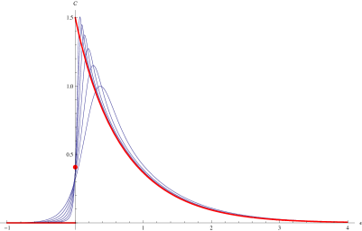
Figure 1: (Colour on-line) $\mathcal{C}(\varepsilon,N)$ versus $\varepsilon$, with $\varepsilon=(K-K_{c})/K_{c}$ for finite $N=32$, $64$, $128$ $256$, $512$, $1024$ (increasing blue curves) and the complete graph limit case $N\to\infty$ (red thick curve). The red dot is the limit at $\varepsilon=0$.

IV The 5-dimensional case

We now come to our Monte Carlo results for $d=5$. As noted in Lundow and Markström (2011) some of the indicators used by other authors to study the critical behaviour for $d=5$ are very sensitive to the exact value of the critical temperature $K_{c}$. With this in mind we will first present a new way of obtaining highly precise estimates for $K_{c}$ and use it to derive the estimate which we will use in our later analysis.

IV.1 An improved method for estimating $K_{c}$

Our improved estimate of $K_{c}$, suitable for $d\geq 4$, is based on a careful study of the magnetisation distribution, i.e. $\Pr(M)$. The approach is simple but assumes that all measurements of $M$ were stored for each temperature during the sampling process. After normalising these values as $x=M/N^{3/4}$ we put them in bins of reasonable width, in our case $0.20$, thus giving us a histogram. There are of course several different binning methods to choose from, but for simplicity we have chosen to use a fixed bin width which is roughly what the Freedman-Diaconis method (twice the interquartile range divided by the cube root of the number of measurements) prescribes when the distribution is near $K_{c}(L)$ (see below) for the weakest data set (i.e. for $L=64$).

The simple distribution density function $f(x)=\phi_{0}\,\exp(\phi_{2}x^{2}+\phi_{4}x^{4})$ is then fitted to this histogram. Since $\phi_{2}$ for all intents and purposes depends linearly on $K$ inside the scaling window (see Fig. 3 of Lundow and Rosengren (2013)), we fit a straight line to the data points (at least seven) on the interval corresponding to $-0.7<\phi_{2}<0.7$ and solve $\phi_{2}(K)=0$. This point constitutes an effective critical temperature $K_{c}(L)$ scaling as $K_{c}(L)-K_{c}\propto L^{2-d}$, see Brezin and Zinn-Justin (1985).

Ideally the density function $f(x)$ should also contain a correction factor $(1+\lambda_{2}x^{2}+\lambda_{4}x^{4}+\lambda_{6}x^{6}+\ldots)$ but the coefficients $\lambda_{i}$ will vanish with increasing $L$. For $L\geq 16$, especially near $K_{c}(L)$, they will not contribute significantly to $f(x)$ and can in any case not be discerned with the data we rely on here. See Lundow and Rosengren (2010, 2013) for a considerably more detailed study of the scaling behaviour of the magnetisation distribution.

In Figure 2 we show $K_{c}(L)$ versus $1/L^{3}$ together with an inset showing the $M/N^{3/4}$-distribution for $L=32$ at different values of $K$ and another inset showing how $\phi_{2}$ depends on $K$ for the different system sizes. A line fit gives that $K_{c}(L)=0.11391498(2)-0.0654(2)\,L^{-3}$. The coefficients and their error estimates are here based on the median and interquartile range of the fitted coefficients when deleting each data point in turn from the line fit. The estimate $K_{c}=0.11391498(2)$ is within the error bars of earlier estimates Luijten et al. (1999); Blöte and Luijten (1997) but adds another digit to the accuracy. This technique for estimating $K_{c}$ is quite robust to variations in the various parameters. For example, changing the distribution bin widths to $0.15$ or using $\phi_{2}$ data for $-0.6<\phi_{2}<0.6$ keeps the resulting $K_{c}$ within the stated error bars.

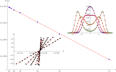
Figure 2: (Colour on-line) $K_{c}(L)$ versus $1/L^{3}$ for $L=16$, $20$, $24$, $32$, $40$, $48$, $56$ and $64$. The fitted line is $0.11391498-0.0654x$. The lower inset shows the fitted parameter $\phi_{2}$ versus $K$ for the same $L$. The upper inset shows the normalised magnetisation distribution $\Pr(M/N^{3/4})$ for $L=32$ at $K=0.1139$, $0.113915$, $0.11393$ and $0.113945$ resulting in $\phi_{2}=-0.251$, $0.036$, $0.323$ and $0.621$ respectively of the fitted $f(x)$ (red curves).

IV.2 Specific heat discontinuity

Consider Figure 3 where we plot the specific heat for $4\leq L\leq 64$ for a wide temperature range. Clearly there is an envelope curve containing the limit specific heat. From the individual $\mathcal{C}(K,L)$ functions we extract the limit function $\mathcal{C}(K,\infty)=\lim_{L\to\infty}\mathcal{C}(K,L)$ from points where the function for increasing $L$ agree. We thus assume that there is a $K_{\min}(L)$ such that if $L^{\prime}\geq L$ and $K>K_{\min}(L)>K_{c}$ then $\mathcal{C}(K,L^{\prime})=\mathcal{C}(K,\infty)$. Analogously we assume there is a $K_{\max}(L)$ such that $\mathcal{C}(K,L^{\prime})=\mathcal{C}(K,\infty)$ when $0<K<K_{\max}(L)<K_{c}$ and $L^{\prime}\geq L$.

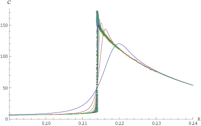
Figure 3: (Colour on-line) $\mathcal{C}(K,L)$ for $L=4$, $6$, $8$, $10$, $12$, $16$, $20$, $24$, $32$, $40$, $48$, $56$ and $64$.

As an example, taking for example $L_{1}=16$ and $L_{2}=20$ we note that $\mathcal{C}(K,16)=\mathcal{C}(K,20)$ when $K>K_{\min}=0.1148$, where $K_{\min}$ of course depends on the chosen $L_{1}$ and $L_{2}$. On the high-temperature side of $K_{c}$ we find that $\mathcal{C}(K,16)=\mathcal{C}(K,20)$ when $K<K_{\max}(16)=0.1120$. Thus we treat the measured data for $\mathcal{C}(K,L)$ as the asymptotic $\mathcal{C}(K,\infty)$ when $L\geq 16$ and $K<0.1120$ or $K>0.1148$. An increasing sequence of pairs of $L_{1},L_{2}$ gives a sequence of $K_{\min}$ and $K_{\max}$ that both approach $K_{c}$. The individual $K_{\min}$ and $K_{\max}$ were found by simply comparing pairwise plots of $\mathcal{C}(K,L)$.

In Figure 4 we show the individual $\mathcal{C}(K,L)$ for $K<K_{\max}(L)$ pieced together into one plot for a range of $L$ and Figure 5 shows the coresponding data for $K>K_{\min}(L)$. Their insets shows the data without removing the finite size behaviour and clearly demonstrate the presence of a limit enveloping curve. Having removed any finite size effects, such as the local maximum for each $L$, the remaining points are in effect estimates of the asymptotic $\mathcal{C}(K,\infty)$ for $0<K<K_{\max}(64)=0.11388$ and $K>K_{\min}(64)=0.11394$.

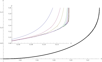
Figure 4: (Colour on-line) $\mathcal{C}(K,L)$ versus $K$ for $K<K_{\max}(L)$ for $L=6$, $8$, $10$, $16$, $20$, $24$, $32$, $40$, $48$, $56$ and $64$. The curve consists of more than 500 points and error bars are not shown. The inset shows a zoomed-in version with 3rd order interpolations through all data points. Data for increasing $L$ start to deviate from envelope curve as we move closer to $K_{c}$.

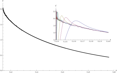
Figure 5: (Colour on-line) $\mathcal{C}(K,L)$ versus $K$ for $K>K_{\min}(L)$ for $L=6$, $8$, $10$, $16$, $20$, $24$, $32$, $40$, $48$, $56$ and $64$.The curve consists of more than 500 points and error bars are not shown. The inset shows a zoomed-in version of 3rd order interpolations through all data points. Data for increasing $L$ deviate from envelope curve as we move closer to $K_{c}$.

In order to estimate the left- and right-limit we take the limit curves and fit a simple expression of the form

$$A_{0}+A_{1}x^{\theta}(1+B_{1}x+B_{2}x^{2}+\ldots)$$ (13)

to $\mathcal{C}(K,\infty)$ where $x=|K-K_{c}|/K_{c}$. We will use $\pm$-superscripts to denote the left- and right-limit as $x\to 0$. This provides left- and right-limits ($A_{0}^{-}$ and $A_{0}^{+}$), the dominating correction term exponents ($\theta^{-}$ and $\theta^{+}$) and a sequence of correction terms. Following Fernández et al. (1992) we call $\theta^{-}$ and $\theta^{+}$ the singular exponents of the specific heat, since they describe the behaviour of the singular part of the specific heat. We are not aware of any prescribed form of the correction terms from earlier studies so these will simply be the effective terms.

Using Mathematica’s built-in FindFit-function we fit the high-temperature limit curve to (13) using both one, two and three correction terms and find excellent agreement in the resulting values of the singular exponent $\theta^{-}$, measuring $\theta^{-}=0.40(1)$. The first two coefficients $A_{0}^{-}$ and $A_{1}^{-}$ also strongly agree when adding more correction terms. However, having first established a strong candidate exponent we now simply fix this to $\theta^{-}=0.4$ and use (13), again trying one, two and three correction terms. Based on this we find an effective fit

$$\mathcal{C}^{-}(x)=0.1697(2)-0.231(1)x^{0.40}(1-0.26(1)x)$$ (14)

where $x=-\varepsilon=(K_{c}-K)/K$ and $0<K<K_{c}$. Adding more correction terms does not improve the fit. The error bars reflect how the coefficients change when adding one or two more terms.

Repeating this exercise for the low-temperature side the FindFit-function suggests $\theta^{+}=0.60(2)$ and again the leading coefficients agree using one, two and three correction terms. Setting $\theta^{+}=0.60$ gives us the effective fit

$$\mathcal{C}^{+}(x)=2.040(1)-2.58(1)x^{0.60}(1-0.36(2)x)$$ (15)

where $x=\varepsilon=(K-K_{c})/K$ and $K>K_{c}$. As before, the error bars reflect how the coefficients change when adding correction terms. We now put (14) and (15) to the test by taking log-log plots of the measured $\mathcal{C}(K,\infty)$ when subtracting the respective limit $A_{0}^{\pm}$.

Beginning with the high-temperature case, in Figure 6 we show $\log(0.1697-\mathcal{C}(K,\infty))$ versus $\log(x)$, where $x=(K_{c}-K)/K_{c}$, together with $\mathcal{C}^{-}(x)$ of (14) (black curve) and the asymptote $0.1697-0.231x^{0.40}$ (red line). The rather small error bars suggest a good quality of the fit. Analogously, on the low-temperature side, we show in Figure 7 $\log(2.04-\mathcal{C}(K,\infty))$ versus $\log(x)$, where $x=(K-K_{c})/K_{c}$, together with $\mathcal{C}^{+}(x)$ of (15) (black curve) and the asymptote $2.04-2.58x^{0.60}$ (red line). For $L=56,64$ the error bars are now quite pronounced. For the smaller $L$ the error bars are considerably more benign.

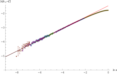
Figure 6: (Colour on-line) $\log(0.1697-\mathcal{C}(K,\infty))$ versus $\log(x)$, with $x=(K_{c}-K)/K_{c}$, for $L=6$, $8$, $10$, $16$, $20$, $24$, $32$, $40$, $48$, $56$ and $64$ (larger $L$ to the left in the figure) together with the fitted $\mathcal{C}^{-}(x)$ (black curve, hard to see) of Eq. (14) and the asymptote $0.1697-0.231x^{0.4}$ (red line with slope $0.40$).

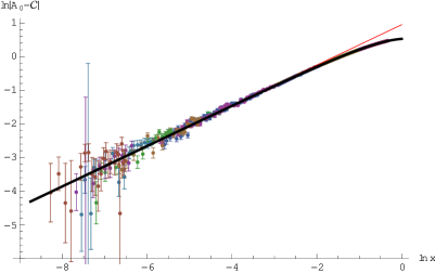
Figure 7: (Colour on-line) $\log(2.04-\mathcal{C}(K,\infty))$ versus $\log(x)$, with $x=(K-K_{c})/K_{c}$, for $L=6$, $8$, $10$, $16$, $20$, $24$, $32$, $40$, $48$, $56$ and $64$ (larger $L$ to the left in the figure) together with the fitted $\mathcal{C}^{+}(x)$ (black curve, hard to see) of Eq. (15) and the asymptote $2.04-2.58x^{0.60}$ (red line with slope $0.60$.

Finally we estimate the value of $\mathcal{C}(K_{c},\infty)$, which, of course, does not have to coincide with any of the $A_{0}^{\pm}$. As it turns out this value is quite distinct from both limits. In Figure 8 we show a zoomed-in plot of $\mathcal{C}(K,L)$ over a range of $L$ for three fixed $K$-values, $K=0.11391498$ (i.e. the estimated $K_{c}$), $K=0.1139148$ and $K=0.1139152$. The $\mathcal{C}(K,L)$ were found by interpolating the data points. As the plot demonstrates, there is a clear upwards trend in the values for $K=0.1139152$ and a clear downwards trend for $K=0.1139148$, whereas the middle value shows no clear trend. A fitted line on the points for $L\geq 16$ suggests $\mathcal{C}(K_{c},\infty)=0.724(3)$. The error bar of this value is obtained by allowing the value of $K$ to vary inside the error bar of $K_{c}$ (2 steps in the 8th digit) and repeat the line fit to the new points.

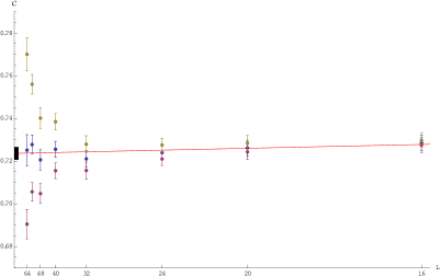
Figure 8: (Colour on-line) $\mathcal{C}(K,L)$ versus $1/L^{5/2}$, for $L=16$, $20$, $24$, $32$, $40$, $48$, $56$ and $64$ together with the fitted red line $0.724+4.19x$, where $x=1/L^{5/2}$. The points trending upwards are for $K=0.1139152$, the points trending downwards are for $K=0.1139148$ and the middle set of points are for $K_{c}=0.11391498$. The rectangle on the $y$-axis indicates the estimate $\mathcal{C}(K_{c},\infty)=0.724(3)$.

The local maximum of $\mathcal{C}(K,L)$, see Figure 5, also takes its own limit value, i.e. $\mathcal{C}_{\max}=\lim_{L\to\infty}\max_{K}\mathcal{C}(K,L)$ does not coincide with the right-hand limit $\mathcal{C}^{-}$. In Figure 9 we show the estimated maximum for each $L$ and the right-hand limit $2.04$ found above (15). It appears very unlikely that they should coincide for large $L$. The fitted line, based on $L\geq 16$, suggests a limit $\mathcal{C}_{\max}=2.225(6)$ where the error bar is based on the variability of the constant term of fitted lines (with $x=1/L^{5/2}$) with one point removed from the data set $L\geq 16$. We estimate that the maximum is located at $K_{\max}=K_{c}+1.860(2)K_{c}/L^{5/2}$, i.e., at $\kappa=1.860(3)$, with the error bar obtained as before by removing individual points for $L\geq 16$ when fitting a line through the origin (since we know $K_{\max}\to K_{c}$). We will plot $\mathcal{C}$ versus $\kappa$ later.

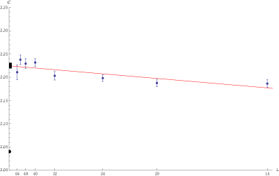
Figure 9: (Colour on-line) $\max_{K}\mathcal{C}(K,L)$ versus $1/L^{5/2}$, for $L=16$, $20$, $24$, $32$, $40$, $48$, $56$ and $64$ together with the fitted red curve $2.225-48.6x$, where $x=1/L^{5/2}$. The rectangle on the $y$-axis indicates the limit estimate $\mathcal{C}_{\max}=2.225(6)$. The point at $y=2.04$ is the right-limit $\mathcal{C}^{+}(0)=2.04$ of Eq. (15).

We can now make a comparison of the behaviour of the 5-dimensional model and that of the mean field case, as derived in the previous section. We first consider the scaling window, in Figure 10 we show a plot of $\mathcal{C}(\kappa)$ for a range of $N$ and the limit case, together with our data for $d=5$. As we can see that maximum specific heat for the mean field limit is lower than the values for $d=5$, but the general shape of the curves are nonetheless quite similar.

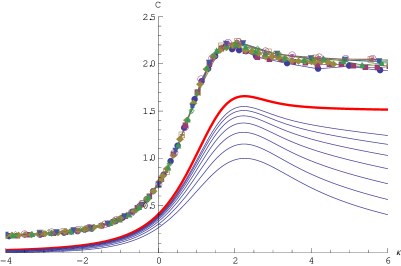
Figure 10: (Colour on-line) $\mathcal{C}$ versus $\kappa$, with $\kappa=\sqrt{N}(K-K_{c})/K_{c}$ for finite $N=32$, $64$, $128$ $256$, $512$, $1024$, $2048$ (increasing blue curves) and the complete graph limit case $N\to\infty$ (red thick curve). The upper set of points shows the same for 5D sampled data points for $L=16$, $20$, $24$, $32$, $40$, $48$, $56$ and $64$. Error bars are shown but of the same size as the points.

Next we look at the thermodynamic limit. In Figure 11 we show the specific heat limit for both the complete graph and $d=5$ in the same plot. As we just noted, the value for the mean field are lower than those for $d=5$ when we are sufficiently close to $\epsilon=0$. We can also see the difference in the singular exponents between the two models, with the mean field case approaching the line $\epsilon=0$ at an angle and the $d=5$ case instead approaching it tangentially.

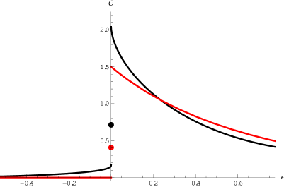
Figure 11: (Colour on-line) The limit specific heat $\mathcal{C}(\varepsilon$ with $\varepsilon=(K-K_{c})/K_{c}$ for the complete graph (red, $y=1.5$, $y=0.407$ and $y=0$ at $y$-axis) and the 5D case (black, $y=2.04$, $y=0.72$ and $y=0.17$ at $y$-axis).

V The model in dimensions 6 and 7

As the dimension $d$ increases we should see the specific heat approach that of the complete graph. We also collected data for $d=6$ and $d=7$ and tried to estimate the singular exponents $\theta^{+}$ and $\theta^{-}$. However, these data rely on considerably smaller systems; $L=4,6,8,10,12,16,20$ for $d=6$ and only $L=4,6,8,10$ for $d=7$. The process is the same as we used above for $d=5$ and we will simply state the resulting estimates of the various parameters.

For $d=6$ we estimate $K_{c}=0.0922982(3)$ and $\mathcal{C}(K_{c},\infty)=0.58(1)$. This value of $K_{c}$ deviates somewhat from the older Monte Carlo estimates, as surveyed in Berche et al. (2008), which have tended to be close to 0.09229, but agrees well with the more recent estimate $0.092298(1)$ Butera and Pernici (2012), coming from the longest series expansion results to date. The limit specific heat is

$$\mathcal{C}=\begin{cases}1.833-2.61\varepsilon^{0.75}(1-0.57\varepsilon)&\varepsilon>0\\ 0.58&\varepsilon=0\\ 0.0927-0.148(-\varepsilon)^{0.60}(1+0.37\varepsilon)&\varepsilon<0\end{cases}$$ (16)

For $d=7$ we estimate $K_{c}=0.0777086(8)$, this is again closer to the series based estimate from Butera and Pernici (2012) than the MC-estimates from Berche et al. (2008), and $\mathcal{C}(K_{c},\infty)=0.53(2)$. The limit specific heat is

$$\mathcal{C}=\begin{cases}1.75-2.47\varepsilon^{0.80}(1-0.56\varepsilon+0.14\varepsilon^{2})&\varepsilon>0\\ 0.53&\varepsilon=0\\ 0.064-0.12(-\varepsilon)^{0.75}(1+0.45\varepsilon)&\varepsilon<0\end{cases}$$ (17)

In both cases the uncertainty in the coefficients is in the last stated digit. Combining $d=5,6,7$ and the complete graph case we plot them all in Figure 12. Inside the scaling window, that is, with respect to $\kappa=\sqrt{N}(K-K_{c})/K_{c}$, we can also clearly see how the specific heat for finite-dimensional systems approach the complete graph limit case. In Figure 13 we plot $\mathcal{C}(\kappa,L)$ for several linear orders $L$ for $d=5,6,7$ and the complete graph.

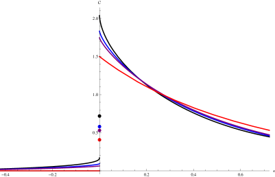
Figure 12: (Colour on-line) The limit specific heat $\mathcal{C}(\varepsilon)$ with $\varepsilon=(K-K_{c})/K_{c}$ for $d=5$ (black), $d=6$ (blue) and $d=7$ (purple) and the complete graph case (red), trending downwards at the $y$-axis, as do the points at $\varepsilon=0$.

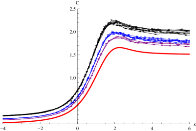
Figure 13: (Colour on-line) The specific heat $\mathcal{C}(\kappa)$ with $\kappa=\sqrt{N}(K-K_{c})/K_{c}$. Trending downwards we see $d=5$ (black, $L\geq 16$), $d=6$ (blue, $L\geq 8$) and $d=7$ (purple, $L\geq 6$) and the complete graph limit (red).

VI Discussion

We have estimated the critical behaviour of the specific heat of the 5-dimensional case and derived the limit curve for the complete graph. The singular exponents for $d=5$ were found to differ for the high- and low-temperature case. To summarise, for $\varepsilon=(K-K_{c})/K_{c}$ we estimate in the 5d case that for $L\to\infty$ the specific heat behaves as

$$\mathcal{C}=\begin{cases}2.040-2.58\varepsilon^{0.60}(1-0.36\varepsilon)&\varepsilon>0\\ 0.724&\varepsilon=0\\ 0.1697-0.231(-\varepsilon)^{0.40}(1+0.26\varepsilon)&\varepsilon<0\end{cases}$$ (18)

The singular exponents are thus $\theta^{+}=0.60$ and $\theta^{-}=0.40$ for $d=5$. As $d\to\infty$ we expect these exponents to approach those of the complete graph where we find $\theta^{+}=\theta^{-}=1$. The exact series expansion of the limit specific heat for the complete graph is

$$\mathcal{C}=\begin{cases}\frac{3}{2}-\frac{12}{5}\varepsilon(1-\frac{73}{70}\varepsilon+\frac{36}{35}\varepsilon^{2}+\cdots)&\varepsilon>0\\ 0.40729006421665228\ldots&\varepsilon=0\\ 0&\varepsilon<0\end{cases}$$ (19)

An open question which would be interesting to settle is how the left and right hand limits of the specific heat for the $d$-dimensional Ising model scales. We expect the limits to approach those of the mean field model as $d\rightarrow\infty$ but we do not yet know how it approaches those values. That the $d\rightarrow\infty$ limit of the value exactly at $K_{c}$ should be the same as the mean field value is far from obvious and would also be worth further investigation. Similarly we would like to know the scaling with $d$ of the left and right singular exponents. We expect both of them to approach 1, but in which way?

VII Acknowledgements

The simulations were performed on resources provided by the Swedish National Infrastructure for Computing (SNIC) at High Performance Computing Center North (HPC2N) and at Chalmers Centre for Computational Science and Engineering (C3SE).

References

- Lundow and Markström (2014) P. Lundow and K. Markström, Nucl. Phys. B 889, 249 (2014).
- Sokal (1979) A. D. Sokal, Phys. Lett. A 71, 451 (1979).
- Aizenman (1981) M. Aizenman, Phys. Rev. Lett. 47, 1 (1981).
- Aizenman (1982) M. Aizenman, Comm. Math. Phys. 86, 1 (1982).
- Aizenman and Fernández (1986) M. Aizenman and R. Fernández, J. Statist. Phys. 44, 393 (1986).
- Sakai (2007) A. Sakai, Comm. Math. Phys. 272, 283 (2007).
- Heydenreich et al. (2008) M. Heydenreich, R. van der Hofstad, and A. Sakai, J. Stat. Phys. 132, 1001 (2008).
- Bollobás et al. (1996) B. Bollobás, G. Grimmett, and S. Janson, Probab. Theory Related Fields 104, 283 (1996).
- Luczak and Luczak (2006) M. J. Luczak and T. Luczak, Random Struct. Algorithms 28, 215 (2006).
- (10) P. H. Lundow and K. Markström, arXiv:1408.2155.
- Fernández et al. (1992) R. Fernández, J. Fröhlich, and A. D. Sokal, Random walks, critical phenomena, and triviality in quantum field theory, Texts and Monographs in Physics (Springer-Verlag, Berlin, 1992), ISBN 3-540-54358-9.
- Lundow and Markström (2011) P. H. Lundow and K. Markström, Nucl. Phys. B 845, 120 (2011).
- Lundow and Rosengren (2010) P. H. Lundow and A. Rosengren, Phil. Mag. 90, 3313 (2010).
- Lundow and Rosengren (2013) P. H. Lundow and A. Rosengren, Phil. Mag. 93, 1755 (2013).
- Brezin and Zinn-Justin (1985) E. Brezin and J. Zinn-Justin, Nucl. Phys. B 257, 867 (1985).
- Luijten et al. (1999) E. Luijten, K. Binder, and H. Blöte, Eur. Phys. J. B 9, 289 (1999).
- Blöte and Luijten (1997) H. W. J. Blöte and E. Luijten, EPL (Europhysics Letters) 38, 565 (1997).
- Berche et al. (2008) B. Berche, C. Chatelain, C. Dhall, R. Kenna, R. Low, and J.-C. Walter, J. Stat. Mech. 2008, P11010 (2008).
- Butera and Pernici (2012) P. Butera and M. Pernici, Phys. Rev. E 86, 011139 (2012).