Self-propelled hard disks: implicit alignment and transition to collective motion

Abstract

We show that low density homogeneous phases of self propelled hard disks exhibit a transition from isotropic to polar collective motion, albeit of a qualitatively distinct class from the Vicsek one. In the absence of noise, an abrupt discontinuous transition takes place between the isotropic phase and a fully polar absorbing state. Increasing the noise, the transition becomes continuous at a tri-critical point. We explain all our numerical findings in the framework of Boltzmann theory, on the basis of the binary scattering properties. We show that the qualitative differences observed between the present and the Vicsek model at the level of their phase behavior, take their origin in the complete opposite physics taking place during scattering events. We argue that such differences will generically hold for systems of self-propelled particles with repulsive short range interactions.

Self-propelled particles borrow energy from their environment and convert it to translational motion. Depending on their density and interaction details, energy taken up on the microscopic scale can be converted into macroscopic, collective motion. A transition from an isotropic phase to a polar, collective phase is observed. Most theoretical knowledge about such active matter and its transitions has been developed for Vicsek-like models: point particles travel at constant speed, to represent self-propulsion, and their interaction rules comprise both explicit alignment and noise, to account for external or internal perturbations. In addition, self-diffusion noise may be incorporated in the individual motion. Typically, the alignment strength and noise intensity control the transition between the isotropic and the polar phases [1, 2, 3, 4, 5, 6].

In order to describe more closely experiments with bacteria [7, 8, 9] or with self-propelled actin filaments [10], other models incorporates the alignment mechanism through the steric interaction of elongated objects [11, 12, 13]. The interaction accounts for the body-fixed axis of these particles, which is in some sense more microscopic than the purely effective (mesoscopic) alignment rules in Vicsek-like models. Steric interaction is not the only microscopic interaction that can lead to collective behaviour. An alternative way to use dynamics for aligning (hard or soft) circular disks is to incorporate inelasticity or softness in the interaction rules [14, 15, 16, 17]. Not surprisingly, also these models exhibit a transition to a globally aligned phase.

A model experimental system of self-propelled disks has been realized by vertically vibrating millimeter-sized circular metal disks with two different “feet” [18, 19]. When isolated, such particles advance in the direction of their body axis, with a reasonably high persistence length. When sufficiently crowded, they start to align to each other and move along in dense clusters. Successful modelling of this experiment, in the form of Newton’s equations for rigid disks with a force acting on the center and a torque turning it around, plus slightly inelastic collisions and some active noise included, have demonstrated that purely repulsive mechanical interaction with no explicit alignment, were sufficient ingredients to observe a transition to collective motion [20]. The nature of this effective alignment remains however mysterious. Is inelasticity a required ingredient? Or, as suggested in [18, 19, 20], does it come from repeated recollisions of particle pairs, during which the velocity vector repeatedly converges against the body axis, but also the body axis has time to relax towards the time-average of the velocity axis. Given that the experiment is very much the one closest to a simple hard-disk liquid and lends itself to a description in terms of statistical physics, understanding precisely its phase transitions, the effective alignment mechanism, and the role of the noise would be a major step towards a theoretical description of active liquids in general.

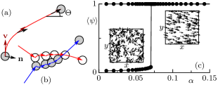
Figure 1: (a) An isolated self-propelled particle converges to its stationary state where velocity ${\mathbf{v}}$ and polarity ${\mathbf{\hat{n}}}$ are parallel. (b) A single binary “scattering event” can consist of many hard-disk elastic collisions. (c) Stable phases in the absence of noise. Between isotropic ($\langle\psi\rangle\approx 0$) and polar ($\langle\psi\rangle=1$) phase is a discontinuous transition.

In this letter we provide such an understanding, restricting ourselves to the analysis of spatially homogeneous phases in the low density limit. To do so we proceed in three steps. (i) We perform molecular dynamics of the model equations for purely elastic interactions, with and without noise: In the absence of noise, the system exhibits a strongly first order transition from the isotropic to the collective motion phase (see Fig. 1c). Above a finite level of noise, the transition becomes second order – a tricritical point exists. This establishes the phase behaviour which we will explain from theoretical considerations. (ii) We analyze the model equations on the grounds of the Boltzmann equation, by making use of a recently proposed observable $\langle{\mathbf{p}\cdot\delta\mathbf{p}}\rangle$ which quantifies the non-conservation of momentum [21]. This observable allows to span the bridge from the microscopic dynamics, in particular binary collisions such as depicted in Fig. 1b, to macroscopic order parameters. From a direct sampling of all possible binary scattering events, we obtain an excellent quantitative prediction of our numerical findings. (iii) We scrutinize the very peculiar dynamics of a collision between two self propelled disks and explain the specific shape of the scattering function that was obtained numerically in (ii). We further find that recollisions are not necessary for the observed alignment, contrary to our previous belief.

0.1 Model of self-propelled hard disks

The model consists of $N$ hard disks in a square box of size $L\times L$, with periodic boundary conditions. The density is $\rho=N/L^{2}$. Particles, being self-propelled, relax to a stationary speed $v_{0}$. As units of length and time we choose the diameter $d_{0}$ of the particles and $d_{0}/v_{0}$, respectively. A particle $i$ has coordinates ${\mathbf{r}}_{i}$, velocity ${\mathbf{v}}_{i}$, and a body axis given by the unit vector ${\mathbf{\hat{n}}}_{i}$ (see Fig. 1a). Between collisions, it evolves according to the equations

$$\tfrac{\text{d}}{\text{d}t}{\mathbf{r}}_{i} ={\mathbf{v}}_{i},$$ (1a)

$$\tau_{v}\tfrac{\text{d}}{\text{d}t}{\mathbf{v}}_{i} ={\mathbf{\hat{n}}}_{i}-{\mathbf{v}}_{i},$$ (1b)

$$\tau_{n}\tfrac{\text{d}}{\text{d}t}{\mathbf{\hat{n}}}_{i} =({\mathbf{\hat{n}}}_{i}\times\hat{\mathbf{v}}_{i})\times{\mathbf{\hat{n}}}_{i}.$$ (1c)

The competition between the self-propulsion ${\mathbf{\hat{n}}}$ and the viscous damping $-{\mathbf{v}}$ in Eq. (1b) lets the velocity relax to ${\mathbf{\hat{n}}}$ on a timescale $\tau_{v}$. Similarly, in Eq. (1c), the polarity ${\mathbf{\hat{n}}}$ undergoes an overdamped torque that orients it toward ${\mathbf{v}}$ on a timescale $\tau_{n}$. Interactions between particles are elastic hard-disk collisions which change ${\mathbf{v}}$ but not ${\mathbf{\hat{n}}}$. After such a collision, ${\mathbf{v}}$ and ${\mathbf{\hat{n}}}$ are not collinear, and the particles undergo curved trajectories which are either interrupted by another collision (Fig. 1b), or the particles reach their stationary state, where ${\mathbf{v}}={\mathbf{\hat{n}}}$ and the trajectory is straight at a speed $v_{0}=1$ (Fig. 1a). The final direction of ${\mathbf{v}}$ (equal to that of ${\mathbf{\hat{n}}}$) depends on the parameter

$$\alpha=\tau_{n}/\tau_{v},$$ (2)

which can be understood as the persistence of the polarity ${\mathbf{\hat{n}}}$. Linearizing the evolution equations around the stationary state, one can show that the final polar angle is given by the weighted average of the initial angles, $(\theta_{n}+\alpha\theta_{v})/(1+\alpha)$. When $\alpha\ll 1$, ${\mathbf{\hat{n}}}$ is practically always directed along ${\mathbf{v}}$.

On top of the deterministic trajectories given by the Eqs. (1), we add some angular noise by the following procedure. Given a time step $\delta t\to 0$, we rotate ${\mathbf{v}}_{i}$ and ${\mathbf{\hat{n}}}_{i}$ by the same angle $\eta_{i}(t)$, distributed normally with zero mean and variance $2D\delta t$, where the constant $D\geq 0$ fixes the level of the angular noise. Noises of different particles are statistically independent. We choose $\delta t$ much smaller than all other timescales in the dynamics. The relevant parameter to characterize the angular noise is then $D/\lambda$, where $\lambda=4\rho/\pi$ is the characteristic scattering rate of the system, which is proportional to the density [21].

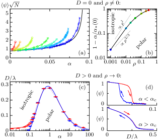
Figure 2: (a) Order parameter in the isotropic phase, without angular noise. $N=1000$ (circles) and $4000$ (crosses). From right to left: theory at $\rho\to 0$, $\rho=10^{-3}$, $0.01$, $0.02$, $0.05$, $0.1$, $0.2$, $0.3$. (b) Dependence of the isotropic–polar transition on the density, with no angular noise. (c) Transition lines in the $(\alpha,D/\lambda)$-plane, at fixed density $\rho=0.01$. Solid lines are theoretical results at $\tau_{v}=\infty$. Upward triangles (red) and downward triangles (blue) are transitions measured numerically by respectively increasing and decreasing $D/\lambda$ quasi-statically. (d) Order parameter obtained by increasing (red) and decreasing (blue) the angular noise.

0.2 Molecular dynamics (MD) simulations

We now establish the phase behaviour of the model for $N$ particles. MD simulations were performed at $\tau_{v}=4$ with $N=1000$ or $N=4000$, focusing on the dilute regime $\rho\ll 1$ (see below for a discussion of the effect of $\tau_{v}$). We are thus left with two microscopic parameters, namely $\alpha$ and $D/\lambda$. Also, the system size is chosen not too large, in order to keep the system spatially homogeneous, which we have checked by visual inspection. We measured the order parameter $\psi(t)=\bigl{|}\sum_{i}{\mathbf{v}}_{i}(t)\bigr{|}/N$, which is of order $1/\sqrt{N}$ for the isotropic state and of order one for the polar state.

Let us first look at the case without angular noise, $D/\lambda=0$. We initialized simulations from random isotropic conditions and waited for the isotropic state to eventually destabilize. When a stationary state was reached, we started to average the order parameter over time, $\langle\psi\rangle$. As shown in Fig. 1c, we found the isotropic state to be stable at low values of $\alpha$, whereas it becomes unstable at larger values, in favour of a polar state. Between the two phases, an abrupt discontinuous transition takes place at $\alpha_{*}$. Quite remarkably, in the whole polar phase the dynamics converges to $\psi=1$, where particles are all strictly parallel. Further, choosing some random state with $\psi\approx 1$ as initial condition, we found that the polar state $\psi=1$ is stable for all $\alpha>0$, in particular also when $\alpha<\alpha_{*}$.

In Fig. 2a, we show again the (now rescaled) order parameter in the isotropic state, this time for different densities. For a given density, the data for different values of $N$ collapse, showing that finite-size effects are under control. In all cases we observed convergence to the fully polar state beyond the points shown. The theoretical framework used below adds the line for $\rho\to 0$, drawn in black. Increasing density here clearly favours the polar state. The departure of the transition due to density effects, $1-\alpha_{*}(\rho)/\alpha_{*}(0)$, is plotted in Fig. 2b.

Adding angular noise to the trajectories quite changes the picture. During simulations we first increased $D/\lambda$ quasi-statically and then decreased it again. The transition was measured by looking at the maximum of the fluctuations of the order parameter among many realizations of the dynamics. The resulting phase diagram at density $\rho=10^{-2}$ is shown in Fig. 2c. In agreement with intuition,the isotropic state is always stable at strong enough angular noise. When decreasing the noise we pass into the polar phase, but the nature of this transition can be either discontinuous or continuous. For values $\alpha<\alpha_{c}\approx 0.157$ the transition has some hysteresis, as indicated in the upper panel of Fig. 2d. The discontinuous nature of the transition is thus robust when adding angular noise, and the phase areas in Fig. 2c overlap, presenting an area which we could call coexistence region if the system were not homogeneous. For $\alpha>\alpha_{c}$, the hysteresis is no longer observed at our level of numerical precision, as can be seen in the lower panel of Fig. 2d. At $\alpha_{c}$, the coexistence zone vanishes into a single line of transition (tricritical point [22, 23, 24]). Interestingly, once in the polar phase, further increasing $\alpha$ leads to a re-entrant transition towards the isotropic phase.

0.3 Kinetic theory framework

We now rationalize these numerical observations in the context of kinetic theory, using the properties of the binary scattering, following Refs. [17, 21]. We summarize here the procedure described in Ref. [21]. In the dilute regime, the mean free-flight time $\lambda^{-1}$ is long enough so that particles have mostly reached their stationary velocity $v_{0}$ before interacting with another particle ($\tau_{v},\tau_{n}\ll\lambda^{-1}$). The binary scattering of self-propelled particles does not conserve momentum, and that is why a polar state can emerge from an isotropic initial condition. Assuming molecular chaos and choosing the von Mises distribution as an ansatz for the angular distribution of the velocities, one can write down an evolution equation for the order parameter $\psi$. This equation can then be expanded, up to order $\psi^{3}$ to study the stability of the isotropic phase [21]:

$$\frac{1}{\lambda}\frac{\text{d}\psi}{\text{d}t}\simeq\bigl{(}\mu-D/\lambda\bigr{)}\psi-\xi\psi^{3},$$ (3)

where the coefficients are given by

$$\mu :=\bigl{\langle}{\mathbf{p}\cdot\delta\mathbf{p}}\bigr{\rangle}_{0},$$ (4)

$$\xi :=\bigl{\langle}(\tfrac{1}{2}-\cos\Delta)\>{\mathbf{p}\cdot\delta\mathbf{p}}\bigr{\rangle}_{0},$$ (5)

$$\langle f\rangle_{0} :=\frac{1}{4}\int_{-1}^{1}\text{d}b\int_{0}^{\pi}\text{d}\Delta\>\Bigl{|}\sin\frac{\Delta}{2}\Bigr{|}f(b,\Delta).$$ (6)

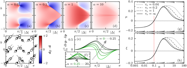
Figure 3: Top: Colour maps of the full scattering function ${\mathbf{p}\cdot\delta\mathbf{p}}(b,\Delta)$. The geometry of the collisions and the colour scale are shown in the bottom-left panel. Bottom–middle: the partially integrated scattering function as a function of the incoming angle $\Delta$, for different values $\alpha$, $\tau_{v}=4$. Right: Fully integrated scattering functions $\mu$ and $\xi$, defined in Eqs. (4) and (5) plotted as a function of $\alpha$ for different $\tau_{v}$. The red vertical line indicates the transition in the absence of noise.

In the stationary state, the left-hand size of Eq. (3) vanishes. The transition line is obtained by solving the equation $\mu(\alpha_{*})=D/\lambda$ for $\alpha_{*}$, while the sign of $\xi(\alpha_{*})$ at the transition tells whether it is continuous or discontinuous. The coefficient $\mu$ is exact within the assumptions of kinetic theory, while $\xi$ should depend on the ansatz used for the angular distribution. Both coefficients are an average over all pre-scattering parameters, as given in Eq. (6), where $b$ is the impact parameter and $\Delta$ is the angle between the incoming particles’ velocities. The averaging needs not be done over the norms of the velocities, since those are fixed to $v_{0}=1$. We have checked explicitly that this assumption holds very well in the numerical simulations in the dilute regime. In Eqs. (4) and (5), ${\mathbf{p}}$ is the pre-scattering momentum of the two colliding particles, and $\delta{\mathbf{p}}$ is the change of their momentum by the scattering event. In contrast with Ref. [17], the above equations explicitly identify the forward component of the momentum change ${\mathbf{p}\cdot\delta\mathbf{p}}$, as the proper quantity to describe the alignment in a binary scattering event. The predictions thus depend only on the microscopic details of the deterministic dynamics through the scattering function ${\mathbf{p}\cdot\delta\mathbf{p}}(b,\Delta)$, which we now explore for the model (1).

0.4 Binary scattering

Remind that a scattering event can consist of several, if not many, hard-disk collisions, such as depicted in Fig. 1b. Before the first collision, both particles are taken to be in the stationary state, i.e. ${\mathbf{v}}={\mathbf{\hat{n}}}$. After the collision, we integrate Eqs. (1) numerically until another collision possibly occurs. The binary scattering is considered over when both particles have again reached their stationary state and are heading away from each other. Repeating the procedure in the whole range of initial parameters $(b,\Delta)$ yields the scattering function ${\mathbf{p}\cdot\delta\mathbf{p}}(b,\Delta)$. Figure 3 shows this function for several $\alpha$, as well as its integral over $b$ and the full integrals yielding the coefficients $\mu$ and $\xi$.

Let us stress that ${\mathbf{p}\cdot\delta\mathbf{p}}$ is not changed by the collision itself, which conserves momentum. All (dis)alignment must here come from the relaxation of the post-collisional value of $|{\mathbf{v}}|$ to unity. Fig. 3a–d shows that scattering at low angular separation, small $\Delta$, always creates forward momentum. In other words, two nearly parallel particles that interact become even more parallel, which gives rise to an effective alignment, ${\mathbf{p}\cdot\delta\mathbf{p}}>0$. On the other hand, for small enough $\alpha$, particles that enter in interaction frontally ($\Delta\approx\pi$) tend to disalign, except for special symmetry such as $b\approx 0$. Increasing $\alpha$ favours aligning scattering events until eventually only aligning events remain. This is best summarized by integrating out all parameter dependence except the incoming angle, as is plotted in Fig. 3e,f.

The coefficients $\mu$ and $\xi$ are then obtained by integrating over $\Delta$, with weights prescribed by Eqs. (4) and (5). Their dependences on the microscopic parameters of the dynamics, $\alpha$ and $\tau_{v}$, are shown in Fig. 3g,h. In the absence of noise, the transition occurs for $\alpha=\alpha_{*}$ such that $\mu(\alpha_{*})=0$; $\xi(\alpha_{*})$ is negative, hence the discontinuous transition. When angular noise is added, the transition is obtained by solving the equation $\mu(\alpha_{*})=D/\lambda$. From the shape of the curve $\mu(\alpha)$, one obtains two values $\alpha_{\pm}$, with $\alpha_{-}\to\alpha_{*}$ and $\alpha_{+}\to\infty$ when $D\to 0$. As $D/\lambda$ is increased, $\xi(\alpha_{-})$ eventually becomes positive and the transition turns continuous at a tricritical point $(\alpha_{c},D_{c}/\lambda)$. Note that $\xi(\alpha_{+})>0$: the re-entrant transition is always continuous. Regarding the role of $\tau_{v}$, $\alpha_{-}$ is practically independant on $\tau_{v}$, while $\alpha_{+}$ increases when $\tau_{v}$ decreases. The theoretical predictions are shown as solid lines in Fig. 2c. The agreement with the MD simulations data for density $\rho=10^{-2}$ is excellent. The small shift of the measured transition lines to the left with respect to the theoretical one comes from finite-density effects.

Finally, we also learn from the examination of the scattering maps that, in the absence of noise, the polar phase $\psi=1$ is actually an absorbing phase [25]: this is because all binary scattering events at small $\Delta$ have ${\mathbf{p}\cdot\delta\mathbf{p}}>0$. When all particles in a system are sufficiently parallel, binary scattering events can only align the system more. This is true for all $\alpha$, and most remarkably for $\alpha\to 0$.

Altogether, our kinetic theory description, using the von Mises ansatz for the angular distribution, captures quantitatively all the phenomenology reported in the numerical simulations at low enough density. It however relies on the numerical evaluation of the scattering maps. In the last part of the paper, we would like to provide some intuition on the origin of the peculiar form of these maps. Also, we will elucidate the role of the multiple collisions which can take place during a scattering event.

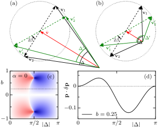
Figure 4: (a,b) Elastic collisions are rotations by an angle $2\beta=2\operatorname{asin}(b)$ in the reference frame of the center-of-mass velocity $\bar{\mathbf{v}}$. Primed quantities (green) are post-collisional, black ones are pre-collisional. (c) The scattering function ${\mathbf{p}\cdot\delta\mathbf{p}}$ resulting from a single collision. (d) A cut through (c) for the value of $b$ used in (a,b).

0.5 Analytical limits

When we take the limit $\tau_{n}\to 0$, the vector ${\mathbf{\hat{n}}}$ has no persistence at all. After two particles collide elastically, the ${\mathbf{\hat{n}}}$ rotate to their respective ${\mathbf{v}}$ instantaneously, the two particles cannot collide a second time and the post-collisional relaxation of $|{\mathbf{v}}|$ to unity occurs on a straight trajectory. We take advantage of this simplification to compute the scattering map in the case $\alpha=0$. Because velocities have equal modulus, we can use the nice visualisation of an elastic collision as a rotation in the center-of-mass frame (Fig. 4a,b). One can then find an analytic expression for ${\mathbf{p}\cdot\delta\mathbf{p}}(b,\Delta)$, which is plotted in Fig. 4c. This plot nicely completes the series of varying $\alpha$ from Fig. 3a-d. The essential structure of the scattering maps can be accounted for by the sole ingredients present in the case $\alpha=0$. Inelastic collisions and persistence of ${\mathbf{\hat{n}}}$ are not essential. Conversely, non-conservation of momentum due to the relaxation of the particle speeds to unity is crucial.

At values $\alpha>0$, the vector ${\mathbf{\hat{n}}}$ has non-vanishing persistence, which results in curved trajectories and possible recollisions. This could lead to the effective alignment mechanism which was proposed to be at the root of the collective motion in the experiment of vibrated polar disks [18, 19, 20]. Concerning the influence of recollisions in the scattering, we ask whether they contribute significantly to $\mu$ and $\xi$. In particular, how numerous are they depending on the scattering geometry $(b,\Delta)$, what is their statistical weight and how much do they affect the scattering map ${\mathbf{p}\cdot\delta\mathbf{p}}(b,\Delta)$? One can get an intuitive picture of the recollision mechanism looking at a simple case, the symmetric ($b=0$) binary scatterings in Fig. 5a. A first collision makes ${\mathbf{v}}$ rotate from being equal to ${\mathbf{\hat{n}}}$ to pointing away from the other particle. On the following trajectory, ${\mathbf{v}}$ and ${\mathbf{\hat{n}}}$ relax towards each other, on their respective timescales $\tau_{v}$ and $\tau_{n}$. For small enough $\tau_{v}$, the persistence of ${\mathbf{\hat{n}}}$ allows for a recollision to take place, and both vectors get closer to each other from one collision to the next.

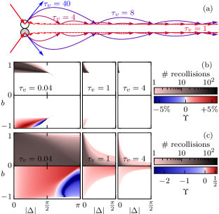
Figure 5: Recollisions. (a) Symmetric binary scatterings for $\alpha=5$. (b, c) Number of recollisions in each scattering (top rows) and their relative contribution to ${\mathbf{p}\cdot\delta\mathbf{p}}$ (bottom rows). $\alpha=0.1$ for (b), $\alpha=10$ for (c).

The highly symmetric case depicted in Fig. 5a is however so degenerate that it has either one or infinite collisions. Unfortunately, the analytic treatment of asymmetric collisions is much too technical to gain physical insight from it and we prefer coming back to the numerical sampling of the scattering events.

For $\alpha=\alpha_{-}$, as shown in Fig. 5b (top row), recollisions can be numerous, but take place only in a small region of the parameter space $(b,\Delta)$, the smaller the larger $\tau_{v}$. We measure their relative contribution to ${\mathbf{p}\cdot\delta\mathbf{p}}$ by $\Upsilon=\tfrac{1}{2}\sin(\Delta/2)({\mathbf{p}\cdot\delta\mathbf{p}}-{\mathbf{p}\cdot\delta\mathbf{p}}|_{1})/|{\mathbf{p}\cdot\delta\mathbf{p}}|$, where ${\mathbf{p}\cdot\delta\mathbf{p}}|_{1}$ is the contribution of the first collision only. As shown in Fig. 5b (bottom row), even for the smallest value $\tau_{v}=0.04$, this contribution is locally less than 5 %. For larger $\tau_{v}$, the contribution is vanishingly smaller. Thus, recollisions has no practical influence on the transition at $\alpha=\alpha_{-}$. Conversely, as shown in Fig. 5c (top row), for $\alpha=\alpha_{+}$, the number of recollisions is not so large, but they occur for wider ranges of scattering parameters and their relative contribution to ${\mathbf{p}\cdot\delta\mathbf{p}}$ is significant, see Fig. 5c (bottom row). This is all the more true for smaller $\tau_{v}$ and is responsible for the dependance of $\mu$ and $\xi$ on $\tau_{v}$ in this regime.

0.6 Discussion

Let us recast our main findings and the understanding we obtained from the above analysis. A homogeneous system of self propelled hard disks, obeying the minimal deterministic Eqs. (1), exhibits a sharp discontinuous transition from an isotropic to an absorbing polar collective motion state, when increasing the persistence of the body axis vector ${\mathbf{\hat{n}}}$. Adding angular noise, the transition becomes continuous via a tricritical point. At fixed noise level, increasing further the persistence of the body axis vector, a re-entrant continuous transition from the polar state to the isotropic state occurs.

All these macroscopic behaviours can be understood by the study of the scattering maps ${\mathbf{p}\cdot\delta\mathbf{p}}$, which describe the level of alignment of all possible scattering events. The most striking feature of these maps is that scattering at low angular separation always creates forward momentum. This is even true for $\alpha=0$, for which, we could prove it explicitly from a mechanical analysis of the collisions. This feature explains the stability of the polar phase in the absence of noise. For small $\alpha$, the dis-alignment, present in the frontal collisions is strong enough to stabilize the isotropic state. For $\alpha>\alpha_{*}$, this does not hold anymore, and the isotropic state becomes unstable. The coexistence of stability of the two states for $\alpha<\alpha_{*}$ guarantees the transition to be discontinuous.

The effect of noise is most easily understood from the shape of the curves $\mu(\alpha)$ and $\xi(\alpha)$. The key point here is that in the present scheme of approximation – Boltzmann equation plus von Mises Ansatz – the computation of $\xi$ is identical to that of $\mu$, apart from the additional asymmetric factor $(1/2-\cos\Delta)$. This does not rely on the specificity of the microscopic model. As a result, the curve $\xi(\alpha)$ is similar to the curve $\mu(\alpha)$, with a shift towards larger $\alpha$. Adding noise simply shifts the transition towards larger $\alpha$: at some point $\xi$ changes signs at the transition, which becomes continuous, hence the tricritical point.

Finally, the re-entrant transition from polar back to isotropic at large $\alpha$ (while increasing $\alpha$) is a direct consequence of the non-monotonous shape of $\mu(\alpha)$. At moderate $\alpha$, the effective alignment $\mu$ increases with the persistence of ${\mathbf{\hat{n}}}$. However, a too large persistence reduces the alignment, because the scattering event does not reorient ${\mathbf{\hat{n}}}$ significantly, and no memory of the collision is kept: ${\mathbf{v}}$ relaxes to practically the same ${\mathbf{\hat{n}}}$ as before the scattering. Some alignment still takes place but is most easily destroyed by small amounts of noise. Interestingly, while the recollisions play no role at the first transition from the isotropic to the polar state, they here increase the effective alignement and thereby postpone the re-entrant transition to larger $\alpha$.

As can be seen from the above discussion, the results do not depend on the details of the scattering maps, as long as binary scattering at low angles produces effective alignment. The partially integrated scattering function (Fig. 3e,f) is then positive for small angles. Models which fall into this class are (i) the here described hard disks with ${\mathbf{v}}$ and ${\mathbf{\hat{n}}}$, (ii) the inelastically colliding hard disks with only ${\mathbf{v}}$ [21], and (iii) the soft disks described in Ref. [17]. All three are self-propelled in the sense that their free-flight speed relaxes to $v_{0}$.

It is important to note that the distinctive behaviour of the above class of system is markedly different from the original Vicsek model, in which binary scattering at low angle effectively disaligns. In the Vicsek model, the partially integrated scattering function [21, Fig. 2a] behaves precisely in the opposite way of the one here. It is therefore unlikely that a coarse-graining of self-propelled hard disks (or any of the above three models) would yield the Vicsek model. Altogether, the present new class of models, including the self-propelled hard particles, could well play for the theory of “simple active liquids” the role that hard spheres play for the statistical mechanics of gases.

References

- [1] \NameVicsek T., Czirók A., Ben-Jacob E., Cohen I. Shochet O. \REVIEWPhys. Rev. Lett.7519951226.
- [2] \NameToner J. Tu Y. \REVIEWPhys. Rev. Lett.7519954326.
- [3] \NameBertin E., Droz M. Grégoire G. \REVIEWPhys. Rev. E74200622101.
- [4] \NameChaté H., Ginelli F., Grégoire G. Raynaud F. \REVIEWPhys. Rev. E772008046113.
- [5] \NameIhle T. \REVIEWPhys. Rev. E832011030901.
- [6] \NamePeshkov A., Bertin E., Ginelli F. Chaté H. \REVIEWEur. Phys. J. Special Topics22320141315.
- [7] \NameZhang H. P., Be’er A., Smith R. S., Florin E. L. Swinney H. L. \REVIEWEPL (Europhysics Letters)87200948011.
- [8] \NameZhang H. P., Be’er A., Florin E. L. Swinney H. L. \REVIEWProceedings of the National Academy of Sciences of the United States of America107201013626.
- [9] \NameChen X., Dong X., Be’er A., Swinney H. L. Zhang H. P. \REVIEWPhys. Rev. Lett.1082012148101.
- [10] \NameSchaller V., Weber C., Semmrich C., Frey E. Bausch A. R. \REVIEWNature467201073.
- [11] \NamePeruani F., Deutsch A. Bär M. \REVIEWPhys. Rev. E74200630904.
- [12] \NameBaskaran A. Marchetti M. C. \REVIEWPhys. Rev. E772008.
- [13] \NameGinelli F., Peruani F., Bär M. Chaté H. \REVIEWPhys. Rev. Lett.1042010.
- [14] \NameAranson I. S. Tsimring L. S. \REVIEWPhys. Rev. E712005050901.
- [15] \NameGrossman D., Aranson I. S. Ben-Jacob E. \REVIEWNew Journal of Physics102008023036.
- [16] \NameHenkes S., Fily Y. Marchetti M. C. \REVIEWPhys. Rev. E842011040301(R).
- [17] \NameHanke T., Weber C. A. Frey E. \REVIEWPhys. Rev. E882013052309.
- [18] \NameDeseigne J., Dauchot O. Chaté H. \REVIEWPhys. Rev. Lett.1052010098001.
- [19] \NameDeseigne J., Léonard S., Dauchot O. Chaté H. \REVIEWSoft Matter820125629.
- [20] \NameWeber C. A., Hanke T., Deseigne J., Léonard S., Dauchot O., Frey E. Chaté H. \REVIEWPhys. Rev. Lett.1102013208001.
- [21] \NameNguyen Thu Lam K.-D., Schindler M. Dauchot O. \REVIEWarXiv:1410.45202014.
- [22] \NameChaikin P. M. Lubensky T. C. \BookPrinciples of condensed matter physics (Cambride University Press, Cambride, U.K.) 1995.
- [23] \NameBaglietto G., Albano E. V. Candia J. \REVIEWPhysica A39220133240.
- [24] \NameRomenskyy M., Lobaskin V. Ihle T. \REVIEWarXiv:1406.69212014.
- [25] \NameHinrichsen H. \REVIEWAdv. Phys.492000815.