The Rotation Period and Magnetic Field of the T Dwarf 2MASSI J1047539+212423
Measured From Periodic Radio Bursts

Abstract

Periodic radio bursts from very low mass stars and brown dwarfs simultaneously probe their magnetic and rotational properties. The brown dwarf 2MASSI J1047539+212423 (2M 1047+21) is currently the only T dwarf (T6.5) detected at radio wavelengths. Previous observations of this source with the Arecibo observatory revealed intermittent, 100%-polarized radio pulses similar to those detected from other brown dwarfs, but were unable to constrain a pulse periodicity; previous VLA observations detected quiescent emission a factor of $\sim$100 times fainter than the Arecibo pulses but no additional events. Here we present 14 hours of Very Large Array observations of this object that reveal a series of pulses at $\sim$6 GHz with highly variable profiles, showing that the pulsing behavior evolves on time scales that are both long and short compared to the rotation period. We measure a periodicity of $\sim$1.77 hr and identify it with the rotation period. This is just the sixth rotation period measurement in a late T dwarf, and the first obtained in the radio. We detect a pulse at 10 GHz as well, suggesting that the magnetic field strength of 2M 1047+21 reaches at least 3.6 kG. Although this object is the coolest and most rapidly-rotating radio-detected brown dwarf to date, its properties appear continuous with those of other such objects, suggesting that the generation of strong magnetic fields and radio emission may continue to even cooler objects. Further studies of this kind will help to clarify the relationships between mass, age, rotation, and magnetic activity at and beyond the end of the main sequence, where both theories and observational data are currently scarce.

1. Introduction

The rotation rates of stars and brown dwarfs span a wide range at birth and evolve with age. In Sun-like stars the dominant process controlling this evolution is the loss of angular momentum through magnetized winds (Weber & Davis, 1967), leading to regulated spin-down over time since the stellar dynamo is rotationally driven (Kraft, 1967; Skumanich, 1972; Noyes et al., 1984). At masses well below that of the Sun, however, the spin-down mechanism appears to be both quantitatively and qualitatively different. While cool stars and brown dwarfs generally have spin-down timescales much longer than Sun-like stars, some mid-to-late M dwarfs have extremely long ($\gtrsim$100 d) rotation periods, suggesting that magnetic braking eventually becomes very effective (Irwin et al., 2011; Bouvier et al., 2013, and references therein).

The “ultracool dwarfs” — stars and brown dwarfs with spectral types M7 and later (Kirkpatrick et al., 1999; Martín et al., 1999) — have a magnetic phenomenology that differs dramatically from that of warmer stars (e.g., Morin et al., 2010; McLean et al., 2012; Stelzer et al., 2012; Williams et al., 2014). This difference may be intimately connected with their non-solar spin-down behavior, so it is valuable to investigate the relationship between magnetic activity, rotation, and other stellar parameters in these objects. However, diagnosing magnetic activity in the coolest dwarfs is difficult due to their intrinsic faintness. This is true not only of their photospheric emission but also of their emission in the $\text{H}\alpha$ and X-ray bands that are often used to trace magnetic activity (Gizis et al., 2000; West et al., 2004; Stelzer et al., 2006; Berger et al., 2010). Radio observations offer a solution: while radio emission is not consistently detected in ultracool dwarfs ($\sim$10% detection rate, McLean et al. 2012), when found its luminosity is relatively high, and is seemingly independent of photospheric temperature (Berger et al., 2001; Berger, 2006; Hallinan et al., 2008; Williams et al., 2014). Furthermore, radio-active ultracool dwarfs often emit bright pulses at the rotation period (Hallinan et al., 2006, 2007, 2008; Berger et al., 2009), potentially allowing simultaneous measurement of both magnetic activity and rotation. This is especially important because brown dwarf rotation measurements based on optical/infrared variability are made challenging due to sensitivity limitations and the evolution of cloud structures on timescales comparable to the rotation period (e.g., Metchev et al., 2014).

The brown dwarf 2MASSI J1047539$+$212423 (hereafter 2M 1047$+$21) is the only T dwarf to have been detected in the radio to date. While early radio observations obtained only a flux density upper limit of 45 $\mu$Jy at 8.46 GHz (Berger, 2006), Route & Wolszczan (2012) detected three bright ($\sim$1.5 mJy), left-circularly-polarized radio bursts at 4.3–5.1 GHz over the course of 15 observations with Arecibo spanning 13 months. With the burst detections spread over the whole 13-month campaign, they were unable to determine a periodicity, leaving the rotation rate of this object unconstrained. A subsequent 3-hour VLA observation by Williams et al. (2013) detected quasi-quiescent emission at $\sim$5.8 GHz at a flux density of $16.5\pm 5.1$ $\mu$Jy but did not find any pulses, although the observations were sensitive to ones similar to the Arecibo events.

In this work we present new radio observations of 2M 1047$+$21 (Section 2) that confirm its quiescent detection but also reveal regularly-spaced, polarized radio bursts similar to those observed with Arecibo (Section 3). We interpret the burst periodicity as the object’s rotation period, thereby allowing it to be placed on a rotation/radio-activity diagram, and interpret the properties of the radio emission in a magnetic loop model (Section 4). We conclude that despite the extremely low temperature of 2M 1047$+$21, its magnetic activity shows continuity with that of other ultracool dwarfs, and that radio observations may be a key tool for tracing the relationship between age, rotation, and magnetic activity at and beyond the end of the main sequence (Section 5).

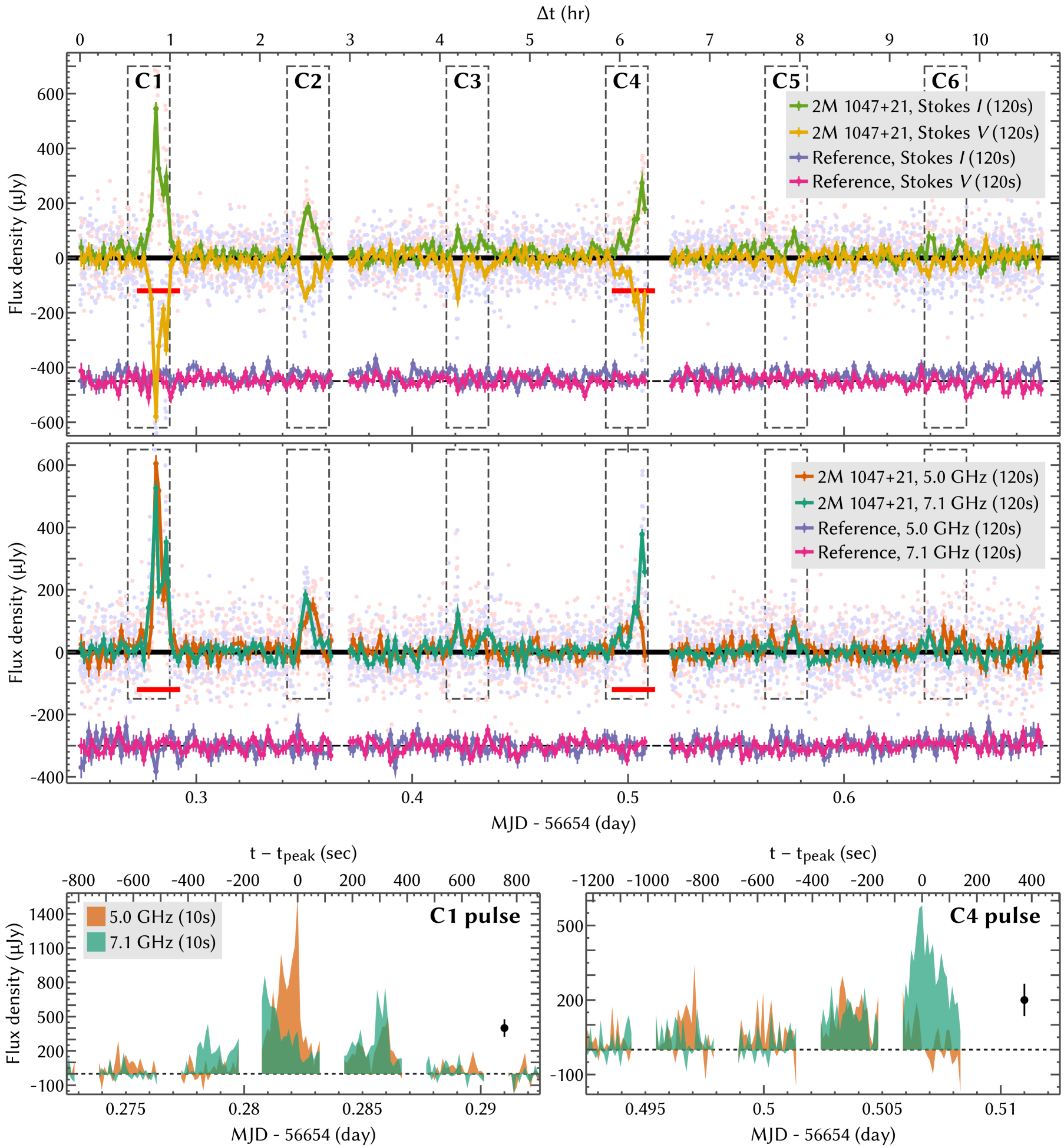
Figure 1.— Top panel: Stokes $I$ and $V$ radio light curves of 2M 1047$+$21 and a reference source (offset for legibility) at 6 GHz. The two 1-GHz-wide spectral windows centered at 5.0 and 7.1 GHz have been averaged together. The faint points show the calibrated data with 10-s sampling, while the heavier points with lines show the data after averaging into 120-s bins. The dashed boxes repeat at the best-fit PDM periodicity of 1.77 hr (Section 3.3) and are 28 minutes wide. Middle panel: Light curves of the two sources with the two spectral windows kept separate, but Stokes parameters averaged to form $\overline{I-V}$. Lower panels: Alternate representation of the unbinned (10-s cadence) $\overline{I-V}$ light curves of 2M 1047$+$21 at the times of the C1 and C4 pulses. The black points show the typical uncertainty of an individual measurement. Horizontal red lines in the upper two panels indicate the time ranges covered by the lower panels.

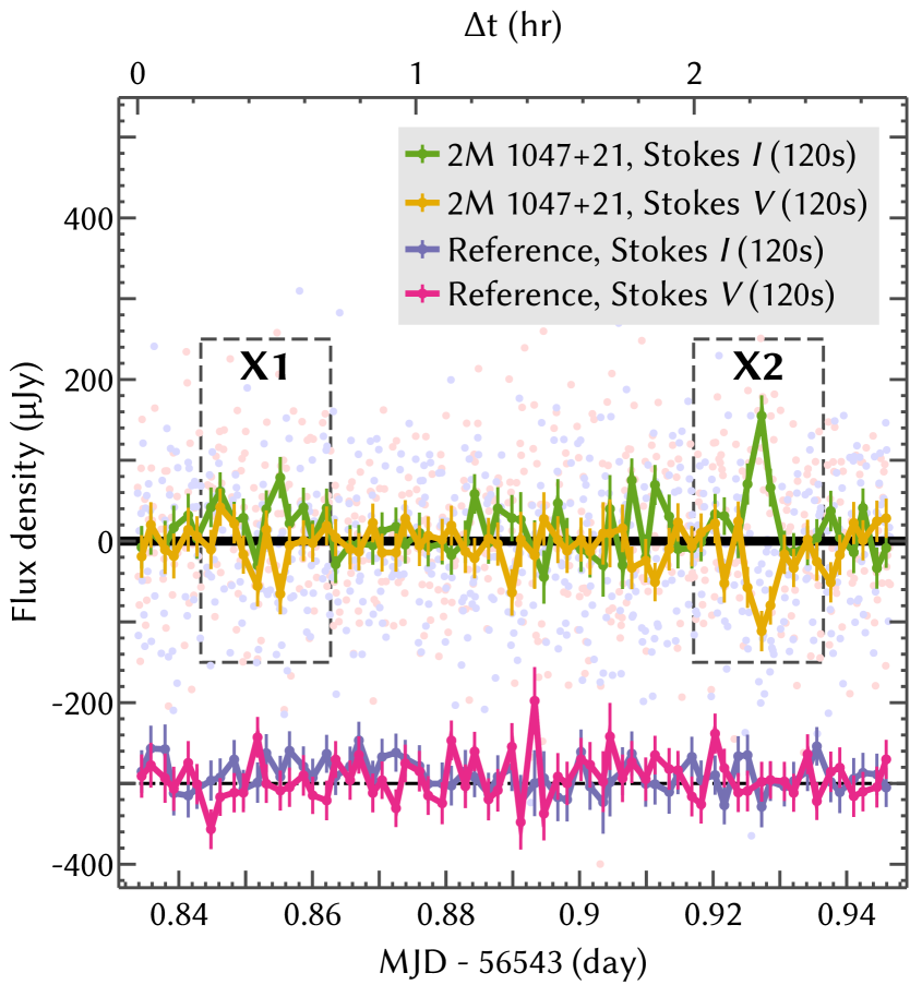
Figure 2.— Stokes $I$ and $V$ radio light curves of 2M 1047$+$21 and a reference source (offset for legibility) in the 9–11 GHz spectral window. Symbols and colors are as in the top panel of Figure 1. Uncalibrated polarimetric leakage terms introduce additional $\lesssim$10% systematic uncertainties into the flux measurements.

2. Observations and Data Reduction

2M 1047$+$21 is a brown dwarf originally identified by Burgasser et al. (1999) with a near-infrared spectral type of T6.5 (Burgasser et al., 2006). Trigonometric parallax measurements reveal a distance of $10.6\pm 0.4$ pc, leading to an estimated $T_{\text{eff}}\sim 900$ K if the radius is assumed to be 0.9 R_J (Vrba et al., 2004). It is one of a few T dwarfs with potential $\text{H}\alpha$ emission, although the detection is marginal at 2.2$\sigma$ (Burgasser et al., 2003a). There is no evidence for 2M 1047$+$21 being a binary system, with high-resolution imaging ruling out companions at separations $\gtrsim$4 AU with mass ratios $\gtrsim$0.4 (Burgasser et al., 2003b).

We observed 2M 1047$+$21 with the Karl G. Jansky Very Large Array (VLA) on 2013 September 8 (UT) for three hours, using the X-band receivers to record data in 1024 spectral channels spanning 9.0–11.0 GHz. We refer to this as the “10-GHz” data set. The flux density and bandpass calibrator was 3C 286 and the complex gain calibrator was the quasar 4C 21.28 (QSO J1051$+$2119). We calibrated the data using standard procedures in the CASA software system (McMullin et al., 2007), automatically flagging radio-frequency interference with the aoflagger tool (Offringa et al., 2010, 2012) using custom VLA-specific settings, and setting the flux density scale to the models of Perley & Butler (2013).

We also observed 2M 1047$+$21 with the VLA on 2013 December 28 (UT) for 11 hours, using the C-band receivers with two spectral windows of 512 channels (1 GHz bandwidth each) centered at 5.0 and 7.1 GHz. We refer to this as the “6-GHz” data set. The same calibrators and analysis methods were used. The calibrator 3C 286 was visited three times over the course of the observation, allowing full polarimetric calibration of the data.

3. The Radio Properties of 2M 1047$+$21

3.1. Images

We image the calibrated visibilities from the 11-hour 6-GHz observation using the CASA imager with multi-frequency synthesis (Sault & Wieringa, 1994) with two Taylor terms and CASA’s multi-frequency CLEAN algorithm. The deep Stokes $I$ image of the field is 2048$\times$2048 pixels with a pixel scale of 0.8^′′ $\times$ 0.8^′′, an effective frequency of 6.05 GHz, and a background rms of 2 $\mu$Jy. We detect a $\sim$12$\sigma$ unresolved source at RA = 10:47:51.95, decl. = $+$21:24:15.7 (ICRS J2000) with a positional uncertainty of 0.2 arcsec in each coordinate and a flux density of $24\pm 3$ $\mu$Jy, where the uncertainty in the flux density is determined from non-linear least squares modeling of the image data. The position is coincident with predictions based on the parallax and proper motion of 2M 1047$+$21 (Vrba et al., 2004), confirming the detection of Williams et al. (2013). Imaging the Stokes $V$ data yields a significant detection with a flux density of $-16\pm 3$ $\mu$Jy, where the negative value indicates left-handed circular polarization (LCP). The spectral index in Stokes $I$ is indistinguishable from zero, $\alpha=0.0\pm 0.3$, where $S_{\nu}\propto\nu^{\alpha}$.

We imaged the calibrated 10-GHz data using the same techniques. We detect a 4.7$\sigma$ source with a flux density of $14\pm 4$ $\mu$Jy at RA = 10:47:51.99, decl. = $+$21:24:15.8 (ICRS J2000), consistent with the C-band detection and astrometric predictions. The Stokes $V$ image exhibits a significant detection with a flux density of $-13\pm 4$ $\mu$Jy, although the lack of polarimetric calibration in this data set decreases the reliability of the measured flux. The Stokes $I$ spectral index is $\alpha=-0.7\pm 0.7$.

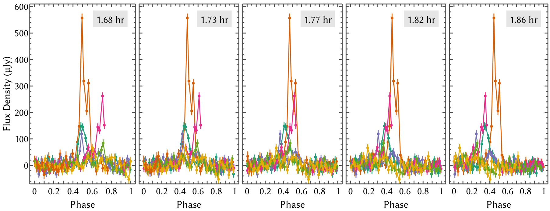
Figure 3.— Frequency-averaged $\overline{I-V}$ light curve of 2M 1047$+$21, phased with different periodicities (labeled within each panel). The central panel phases at the best PDM periodicity of 1.77 hr.

3.2. Light Curves

We extract light curves using the technique described in Williams et al. (2013). The results at 6 and 10 GHz are shown in Figure 1 and Figure 2, respectively. These figures also show the extracted light curve of a nearby, non-variable radio source at RA = 10:47:50.49, decl. = $+$21:24:32.8 for comparison. We detect multiple bright pulses from 2M 1047$+$21 in the 6-GHz observation, and at least one pulse in the 10-GHz observation. Although the profiles of the individual 6-GHz pulses vary, they appear to occur periodically; in Section 3.3, we derive a periodicity of $\sim$1.77 hr. Using this periodicity and the timing of the brightest pulses, we identified eight temporal “windows” of interest in the two data sets shown in Figure 1 and Figure 2. We denote them C1–C6 for the 6-GHz (C-band) data and X1–X2 for the 10-GHz (X-band) data. Their width (28 minutes) and phasing were chosen manually to emphasize the time periods where the radio emission appears most variable. The uncertainty in the periodicity is such that the relative phasing of the windows from the two observations is unconstrained.

Windows C1, C2, C4, and X2 clearly contain radio pulses, but it is less obvious whether the remaining windows do. In the Appendix, we describe our method for evaluating the significance of the source variability in the other windows. We find that the pulses in windows C3 and C5 are significant at the 7.2$\sigma$ and 3.2$\sigma$ levels, respectively. On the other hand, the variations in windows C6 and X1 have significances of 0.8$\sigma$ and 1.0$\sigma$, respectively. While the timing of the events in the last two windows is suggestively close to where the periodic pulses should occur, we cannot reject the null hypothesis that they are noise fluctuations.

Review of Figure 1 reveals some basic characteristics of the 6-GHz pulses. Their amplitudes, temporal profiles, and frequency structure all vary. The variations during the brightest (C1) pulse indicate that the pulse intensity can modulate on timescales shorter than the 10 s integration time of the underlying data (Figure 1, bottom-left panel), as supported by prior Arecibo observations (Route & Wolszczan, 2012). Considering longer timescales, both double-peaked and single-peaked pulse profiles are seen; the variation in pulse profile is more abrupt than that seen in other ultracool dwarfs with periodic radio bursts (Hallinan et al., 2006, 2007, 2008; Berger et al., 2009). In the 5.0 GHz frequency window, the peak observed pulse flux density reaches $1550\pm 90$ $\mu$Jy, comparable to the events reported by Route & Wolszczan (2012). The most well-constrained pulse durations are those of the brightest parts of pulses C1 and C4, which are 500–800 s.

The frequency structure of the pulses also varies. In most cases, the amplitudes of the 5.0 and 7.1 GHz profiles are approximately equal, but the high-frequency component of pulse C4 is $\sim$3 times as bright as the low-frequency component. The timing between the two frequency windows varies as well. In pulse C1, the 7.1 GHz portion peaks $\sim$130 s before the 5.0 GHz portion. Treating this separation as a frequency drift in a single underlying pulse implies a drift rate of 16 MHz s^-1, more than an order of magnitude lower than that inferred by Route & Wolszczan (2012). However, in other windows (e.g., C3) there is no discernable lag between the low and high frequency windows, and in C4 the first low-frequency peak (MJD 56654.497) leads the high-frequency emission ($56654.502<\text{MJD}<56654.508$; Figure 1, bottom-right panel). Based on the more sensitive observations of Route & Wolszczan (2012), which resolve the radio bursts of 2M 1047$+$21 into individual pulses lasting tens of seconds, the frequency-dependent variations seen on the $\sim$120-s timescales over which we average should probably not be taken to trace the evolution of single pulse.

In most cases the pulses are $\sim$100% LCP, although there is some variation in the fractional circular polarization down to $\sim$50% LCP. In the subsequent analysis of the pulse intensities we consider the weighted average of $I$ and $-V$, denoted $\overline{I-V}$, which averages the LCP component and any unpolarized contribution.

We computed the quiescent flux density of 2M 1047$+$21 by time averaging the light curve outside of the boxed regions shown in Figure 1. We find Stokes $I$ and $V$ flux densities of $9.3\pm 1.5$ and $1.1\pm 1.5$ $\mu$Jy, respectively. The quiescent circular polarization level is $-6\%\lesssim p\lesssim 28\%$, where negative values imply LCP and positive values RCP.

3.3. Periodicity

We derive a periodicity for the frequency-averaged $\overline{I-V}$ component of the 6-GHz light curve data using the phase dispersion minimization technique (PDM; Stellingwerf, 1978), in which the data are placed into phase bins and the overall scatter within each bin is summarized with a statistic denoted $\Theta$. The best-fit periodicity, namely the one that minimizes $\Theta$, is $P\sim 1.77$ hr (with $\Theta=0.79$).

A standard method for assessing the significance of a PDM result is to compare the value of $\Theta$ obtained from the actual data to the distribution of $\Theta$ values obtained from random permutations of the data. Applied here, this approach suggests that the significance is high; in 10,000 trials with randomly-permuted copies of the data, none achieved a $\Theta$ statistic as low as the one actually obtained. However, it is not obvious that this metric is appropriate for these data, where the pulse profile must be highly variable for the PDM periodicity to hold. We investigated the significance of the periodicity using an additional Monte Carlo method. Consider a sequence of periodic events with their timing defined by a periodicity $P$ and a dimensionless phase $\phi$. The dimensionless separation between a time $t$ and the nearest event is

$$\delta(t)=\left[\left(\frac{t}{P}-\phi\right)\bmod 1\right]-\frac{1}{2},$$ (1)

where by definition $-1/2\leq\delta<1/2$. We can leverage this definition to define a total “distance” between a set of times $t_{i}$ and a given periodic sequence:

$$\Delta^{2}=\sum_{i}\delta(t_{i})^{2}.$$ (2)

Using a Levenberg-Marquardt algorithm to minimize $\Delta^{2}$ as a function of $P$ and $\phi$, we found $\Delta^{2}=0.016$ for pulses C1–C5. The algorithm was initialized with $P$ approximately equal to the mean interpulse spacing, avoiding convergence to arbitrarily small values of $\Delta^{2}$ with $P\to 0$. We performed the same kind of minimization with 50,000 sets of five pulses occurring at times chosen uniformly randomly in the range $56654.2468<\text{MJD}<56654.6300$, representing the time range in which the five significant 6-GHz pulses are observed. Only 1.8% of these Monte Carlo realizations had $\Delta^{2}<0.016$, strengthening the case that the periodic appearance of the pulses is not due to random chance.

A Monte Carlo assessment of the PDM period uncertainty based on adding noise to the data results in a measured periodicity of $1.771\pm 0.001$ hr, but the true uncertainty on this value is higher because the of the variable pulse profile. In Figure 3 we show the light curve data phased to several periods close to the PDM result. From visual inspection of these phasings, we estimate that the uncertainty in the period is $\sim$0.04 hr. The low-significance X1 peak in the 10-GHz data at MJD 56543.855 occurs $\sim$1.73 hr before the prominent peak at MJD 56543.927, providing tentative evidence that the periodic pulsing behavior may extend to higher frequencies.

4. Discussion

Although our previous observations of 2M 1047$+$21 were equally sensitive to radio pulses and lasted for $\sim$1.6 pulse periods (Williams et al., 2013), no pulses were detected. Route & Wolszczan (2012) detected pulses only intermittently in their observations as well, and similar intermittency has been also observed in multi-rotation observations of the M8.5 dwarf TVLM 513 separated by about a year (Hallinan et al., 2007; Berger et al., 2008). Order-of-magnitude variations in the quiescent radio emission of the L2.5 dwarf 2MASS J05233822$-$1403022 has also been reported to occur on month-to-year timescales (Antonova et al., 2007). Overall, there is evidence for significant variability in ultracool dwarf radio emission on both short time scales and long ones. The available data are insufficient, however, to provide even a basic quantitative characterization of the nature of the long-term variability. While insight into the long-timescale evolution of related processes can be gained through monitoring of flares and spot evolution in optical/IR campaigns (e.g., Gizis et al., 2013), sustained radio monitoring is essential. The magnitude and prevalence of this variability further implies that out of the ultracool dwarfs (including T dwarfs) that were not detected in prior radio surveys (Berger, 2006; McLean et al., 2012) a substantial fraction may in fact be intermittent radio emitters.

It is apparent from Figures 1–2 that the pulse amplitudes and profiles vary from one event to the next and also vary with radio frequency within a single event. It is also apparent that the observed 6-GHz pulse peaks do not occur in a strictly periodic fashion. Based on the overall regular timing of the pulses and the significant variability in their profiles (Figure 1), we interpret the lack of a consistent periodicity as being due to variations in the pulse structure from one event to the next, rather than reflecting a genuine aperiodicity in the physical process that drives the overall pulse timing. If commonplace, these variations could significantly complicate attempts to measure the pulse periods of ultracool dwarfs at high precision (e.g., Wolszczan & Route, 2014).

Periodic radio pulses in ultracool dwarfs have been attributed to beamed auroral emission modulated at the rotation period (Hallinan et al., 2006, 2007, 2008; Berger et al., 2009). The characteristics of the pulses in our data — $\sim$100% polarization, frequency drifts, varying pulse amplitude, and double-peaked pulse structures — are fully consistent with those seen in other ultracool radio emitters, and we likewise interpret the pulse periodicity of $\sim$1.77 hr as the rotation period of 2M 1047$+$21. Assuming a radius of $0.9\pm 0.15$ R_J (Vrba et al., 2004) and solid-body rotation, this corresponds to an equatorial rotational velocity of $63\pm 10$ km s^-1. This is just the sixth rotation period measured in a late T dwarf (Koen et al., 2004; Clarke et al., 2008; Buenzli et al., 2012; Radigan et al., 2014; Metchev et al., 2014), and the first to be obtained from radio observations.

In Figure 4, we use this measurement to place 2M 1047$+$21 on a rotation/radio-activity diagram (McLean et al., 2012). In these analyses rotation is typically parametrized with $v\sin i$, for which more measurements are available, so we do this as well, setting $\sin i=1$. We quantify radio activity with both the radio spectral luminosity, $L_{\nu,\text{R}}$, and its ratio to the bolometric luminosity, $L_{\nu,\text{R}}/L_{\text{bol}}$. Although 2M 1047$+$21 is an outlier in the sample of radio-detected ultracool dwarfs for both its low temperature and rapid rotation, its radio activity does not appear to deviate substantially from the trends identified in warmer objects. In particular, $L_{\nu,\text{R}}/L_{\text{bol}}$ in those rapidly-rotating ultracool dwarfs with radio detections appears to increase with rotation, exhibiting no “saturation” or “super-saturation” effects seen in other activity tracers such as $L_{\text{X}}/L_{\text{bol}}$ or $L_{\text{H}\alpha}/L_{\text{bol}}$ (Vilhu, 1984; Randich et al., 1996; McLean et al., 2012; Cook et al., 2014). On the other hand, this effect seems to be almost entirely driven by evolution in $L_{\text{bol}}$; the quiescent radio luminosity of active ultracool dwarfs is generally found to lie in the range $10^{12.5}<L_{\nu,\text{R}}<10^{13.5}$. It has been argued that this effect is due to the emergence of coherent auroral processes as the source of seemingly quiescent radio emission in the ultracool regime (Hallinan et al., 2008), but standard coronal gyrosynchrotron emission can also explain this result (Williams et al., 2014).

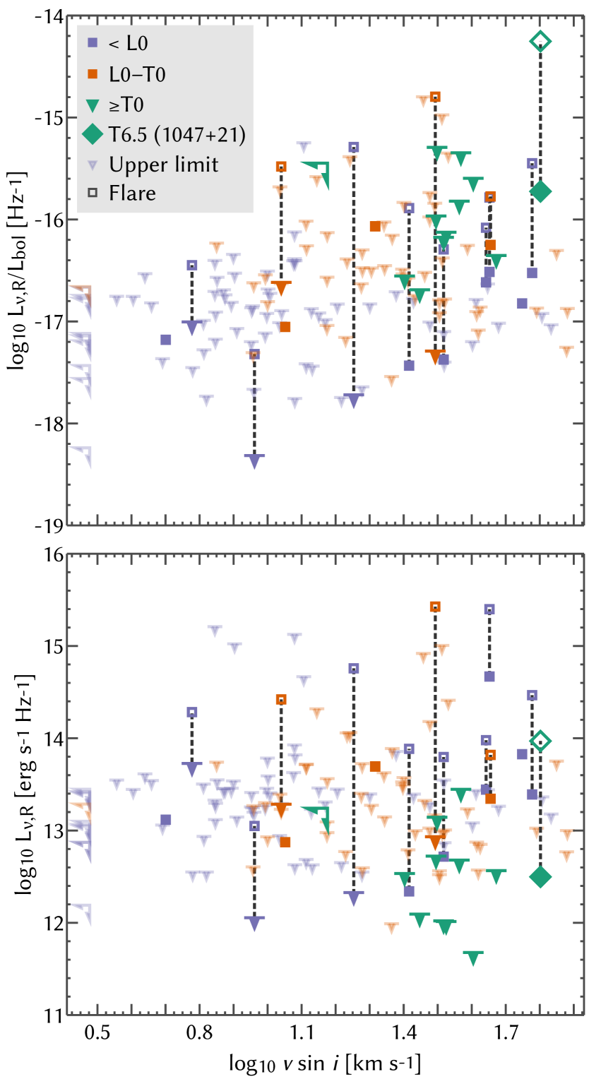
Figure 4.— Relationship between radio emission and rotation in ultracool dwarfs. Rotation is quantified with $v\sin i$. In the upper panel, radio activity is normalized by bolometric luminosity, computed as described in Williams et al. (2014). In the lower panel, un-normalized $L_{\nu,\text{R}}$ is shown. 2M 1047$+$21 is the only T dwarf to be detected in the radio. We have converted its rotation period to $v\sin i$ using $\sin i=1$, so that its true horizontal position may lie to the left of that shown. Assuming a randomly-oriented rotation axis, the most probable offset is $\log_{10}\pi/4\approx 0.1$.

Pulsed (rather than quiescent) radio emission in ultracool dwarfs reaches brightness temperatures that likely require a coherent emission mechanism (Hallinan et al., 2006, 2008; Route & Wolszczan, 2012), and the electron cyclotron maser instability (ECMI; Wu & Lee, 1979; Treumann, 2006) has generally been the best explanation for the data (e.g., Lynch et al., 2014). ECMI emission is dominated by the first harmonic of the cyclotron frequency $\nu_{c}=eB/2\pi m_{e}c$, so that the ECMI spectrum provides a direct measurement of the magnetic field strength at the emission site, which is probably near the surface at the magnetic poles (in analogy with solar system auroral emitters). While there is insufficient evidence to conclude that periodic pulsed emission extends to the 10-GHz data, there is at least one highly-polarized pulse present at these frequencies, and thus we argue that the surface field strength reaches at least $\sim$3.6 kG. There is no evidence for a high-frequency cutoff in the pulse spectrum in the 10-GHz data, so the magnetic field strength may be even larger.

Although our observations are consistent with the model of discrete ECMI-emitting magnetic loops recently investigated by Lynch et al. (2014), they lack some of the features that distinguish this model. In particular, the pulses we observe are consistently LCP, while the discrete loop model provides a natural explanation for pulses with both LCP and RCP peaks, as sometimes observed (Hallinan et al., 2006, 2007). The discrete loop model also provides a natural explanation for observations of multiple pulses per rotation, which do not appear to occur in our data (although we cannot exclude the unlikely possibility that the true rotation period is a multiple of the one that we determine and the pulses arrive evenly spaced in time within each rotation). While our observations are not inconsistent with the discrete loop model, they could also be explained as arising from beamed emission in an auroral oval associated with a global dipolar field (Trigilio et al., 2011; Williams et al., 2015).

A more ambitious interpretation of the 7.1-GHz pulse phasing, however, might lend support to the discrete loop model. The 7.1-GHz maxima of pulses C1–C3 and C4–C5 in Figure 1 are consistently spaced by $\sim$1.68 hr, to be compared to our adopted periodicity of 1.77 hr (Figure 3). Meanwhile the 7.1-GHz maxima of pulses C3 and C4 are separated by 2.05 hr. If the 1.68 hr separation is adopted as the rotation period, an interpretation for this offset could be that the emission in pulses C1–C3 and C4–C5 originates from different loops found at longitudes differing by $\sim$80°. In this scenario a particle acceleration event would have occurred along the second loop some time between pulses C3 and C4, and the decrease in pulse amplitude over time (in windows C1–C3 and C4–C6) suggests that the accelerated particles dissipate their energy over timescales comparable to the rotation period. However, this interpretation requires somewhat implausible timing of events: although it suggests that multiple discrete magnetic loops capable of sourcing observable ECMI emission are present, only one of them is “lit up” at a time, and a new one “lights up” as soon as the the old one fades. Furthermore, the timing of the 5 GHz peaks does not provide as much support for the model of a shorter rotation period and phase jump.

5. Conclusions

Our VLA observations of 2M 1047$+$21 confirm our previous quiescent detection (Williams et al., 2013) and demonstrate that its emission extends up to at least $\sim$10 GHz. The prominent polarized radio bursts in our data confirm the results of Route & Wolszczan (2012); the lack of such pulses in our prior observations, which would have detected them, provides further evidence that the radio emission of ultracool dwarfs is variable on time scales long compared to the rotation period (Antonova et al., 2007; Hallinan et al., 2007; Berger et al., 2008), in addition to the apparent short-timescale variation. We use the pulses to measure a rotation period of 1.77 hr with an uncertainty of about 0.04 hr (Figure 3). These findings highlight the advantages of the VLA over Arecibo for these studies: as a high resolution interferometer it is much more sensitive to faint quiescent emission, and its ability to point all over the sky allows long observations that can detect multiple pulses in sequence, yielding rotation period measurements.

The coherent, periodic radio bursts we observe are consistent in many ways with the emission from other ultracool dwarfs. In particular, despite the extremely low temperature ($\sim$900 K) of this brown dwarf, we infer that its surface magnetic field strength is at least 3.6 kG. Magnetic fields appear to be generated and dissipated in a consistent way in ultracool dwarfs in spectral types ranging from $\sim$M7 through at least T6.5, at least in the population of radio-detected objects, which consists of $\sim$10% of the general sample (McLean et al., 2012). This result is promising in the context of future radio studies of exoplanets.

Our findings demonstrate the potential of radio observations to reveal how (sub)stellar rotational evolution proceeds at the bottom of the main sequence. Studies of the relationships between mass, rotation, age, and magnetic activity disagree as to the underlying processes (e.g., Reiners & Mohanty, 2012; Gallet & Bouvier, 2013; Matt et al., 2014) and have thus far provided only weak constraints in the brown dwarf regime (Bouvier et al., 2013, and references therein). Radio observations offer two advantages at the lowest masses. First, they can simultaneously probe both rotation and magnetic activity, and in fact are one of the few effective means of probing magnetism in the brown dwarf regime at all (McLean et al., 2012). Second, radio measurements of rotation periods are relatively precise, while measurements from variability in the optical and infrared are made ambiguous by sensitivity limitations and the evolution of cloud structures on timescales comparable to the rotation period (e.g., Metchev et al., 2014). In order to realize the potential of radio studies, however, systematic efforts are needed to discover more radio-emitting ultracool dwarfs and understand the origins of their radio activity.

References

- Antonova et al. (2007) Antonova, A., Doyle, J. G., Hallinan, G., Golden, A., & Koen, C. 2007, A&A, 472, 257
- Astropy Collaboration et al. (2013) Astropy Collaboration, Robitaille, T. P., Tollerud, E. J., et al. 2013, A&A, 558, 33
- Berger (2006) Berger, E. 2006, ApJ, 648, 629
- Berger et al. (2001) Berger, E., Ball, S., Becker, K. M., et al. 2001, Natur, 410, 338
- Berger et al. (2008) Berger, E., Gizis, J. E., Giampapa, M. S., et al. 2008, ApJ, 673, 1080
- Berger et al. (2009) Berger, E., Rutledge, R. E., Phan-Bao, N., et al. 2009, ApJ, 695, 310
- Berger et al. (2010) Berger, E., Basri, G., Fleming, T. A., et al. 2010, ApJ, 709, 332
- Bouvier et al. (2013) Bouvier, J., Matt, S. P., Mohanty, S., et al. 2013, to appear in proceedings of Protostars & Planets VI, arxiv:1309.7851
- Buenzli et al. (2012) Buenzli, E., Apai, D., Morley, C. V., et al. 2012, ApJL, 760, L31
- Burgasser et al. (2006) Burgasser, A. J., Geballe, T. R., Leggett, S. K., Kirkpatrick, J. D., & Golimowski, D. A. 2006, ApJ, 637, 1067
- Burgasser et al. (2003a) Burgasser, A. J., Kirkpatrick, J. D., Liebert, J., & Burrows, A. 2003a, ApJ, 594, 510
- Burgasser et al. (2003b) Burgasser, A. J., Kirkpatrick, J. D., Reid, I. N., et al. 2003b, ApJ, 586, 512
- Burgasser et al. (1999) Burgasser, A. J., Kirkpatrick, J. D., Brown, M. E., et al. 1999, ApJL, 522, L65
- Clarke et al. (2008) Clarke, F. J., Hodgkin, S. T., Oppenheimer, B. R., Robertson, J., & Haubois, X. 2008, MNRAS, 385, 2009
- Cook et al. (2014) Cook, B. A., Williams, P. K. G., & Berger, E. 2014, ApJ, 785, 10
- Gallet & Bouvier (2013) Gallet, F., & Bouvier, J. 2013, A&A, 556, 36
- Gizis et al. (2013) Gizis, J. E., Burgasser, A. J., Berger, E., et al. 2013, ApJ, 779, 172
- Gizis et al. (2000) Gizis, J. E., Monet, D. G., Reid, I. N., et al. 2000, AJ, 120, 1085
- Hallinan et al. (2006) Hallinan, G., Antonova, A., Doyle, J. G., et al. 2006, ApJ, 653, 690
- Hallinan et al. (2008) —. 2008, ApJ, 684, 644
- Hallinan et al. (2007) Hallinan, G., Bourke, S., Lane, C., et al. 2007, ApJL, 663, L25
- Irwin et al. (2011) Irwin, J., Berta, Z., Burke, C., et al. 2011, ApJ, 727, 56
- Kirkpatrick et al. (1999) Kirkpatrick, J. D., Reid, I. N., Liebert, J., et al. 1999, ApJ, 519, 802
- Koen et al. (2004) Koen, C., Matsunaga, N., & Menzies, J. 2004, MNRAS, 354, 466
- Kraft (1967) Kraft, R. P. 1967, ApJ, 150, 551
- Lynch et al. (2014) Lynch, C., Mutel, R. L., & Güdel, M. 2014, ApJ submitted, arxiv:1405.3516
- Martín et al. (1999) Martín, E. L., Delfosse, X., Basri, G., et al. 1999, AJ, 118, 2466
- Matt et al. (2014) Matt, S. P., Brun, A. S., Baraffe, I., Bouvier, J., & Chabrier, G. 2014, ApJL in press, arxiv:1412.4786
- McLean et al. (2012) McLean, M., Berger, E., & Reiners, A. 2012, ApJ, 746, 23
- McMullin et al. (2007) McMullin, J. P., Waters, B., Schiebel, D., Young, W., & Golap, K. 2007, in Astronomical Society of the Pacific Conference Series, Vol. 376, Astronomical Data Analysis Software and Systems XVI, ed. R. A. Shaw, F. Hill, & D. J. Bell, 127
- Metchev et al. (2014) Metchev, S., Heinze, A., Apai, D., et al. 2014, ApJ in press, arxiv:1411.3051
- Morin et al. (2010) Morin, J., Donati, J. F., Petit, P., et al. 2010, MNRAS, 407, 2269
- Noyes et al. (1984) Noyes, R. W., Hartmann, L. W., Baliunas, S. L., Duncan, D. K., & Vaughan, A. H. 1984, ApJ, 279, 763
- Offringa et al. (2010) Offringa, A. R., de Bruyn, A. G., Biehl, M., et al. 2010, MNRAS, 405, 155
- Offringa et al. (2012) Offringa, A. R., van de Gronde, J. J., & Roerdink, J. B. T. M. 2012, A&A, 539, A95
- Pedregosa et al. (2011) Pedregosa, F., Varoquaux, G., Gramfort, A., et al. 2011, Journal of Machine Learning Research, 12, 2825
- Perley & Butler (2013) Perley, R. A., & Butler, B. J. 2013, ApJS, 204, 19
- Radigan et al. (2014) Radigan, J., Lafrenière, D., Jayawardhana, R., & Artigau, E. 2014, ApJ, 793, 75
- Randich et al. (1996) Randich, S., Schmitt, J. H. M. M., Prosser, C. F., & Stauffer, J. R. 1996, A&A, 305, 785
- Reiners & Mohanty (2012) Reiners, A., & Mohanty, S. 2012, ApJ, 746, 43
- Route & Wolszczan (2012) Route, M., & Wolszczan, A. 2012, ApJL, 747, L22
- Sault & Wieringa (1994) Sault, R. J., & Wieringa, M. H. 1994, A&AS, 108, 585
- Skumanich (1972) Skumanich, A. 1972, ApJ, 171, 565
- Stellingwerf (1978) Stellingwerf, R. F. 1978, ApJ, 224, 953
- Stelzer et al. (2006) Stelzer, B., Micela, G., Flaccomio, E., Neuhäuser, R., & Jayawardhana, R. 2006, A&A, 448, 293
- Stelzer et al. (2012) Stelzer, B., Alcalá, J., Biazzo, K., et al. 2012, A&A, 537, A94
- Treumann (2006) Treumann, R. 2006, A&ARv, 13, 229
- Trigilio et al. (2011) Trigilio, C., Leto, P., Umana, G., Buemi, C. S., & Leone, F. 2011, ApJL, 739, L10
- Vilhu (1984) Vilhu, O. 1984, A&A, 133, 117
- Vrba et al. (2004) Vrba, F. J., Henden, A. A., Luginbuhl, C. B., et al. 2004, AJ, 127, 2948
- Weber & Davis (1967) Weber, E., & Davis, L. 1967, ApJ, 148, 217
- West et al. (2004) West, A. A., Hawley, S. L., Walkowicz, L. M., et al. 2004, AJ, 128, 426
- Williams et al. (2015) Williams, P. K. G., Berger, E., Irwin, J., Berta-Thompson, Z. K., & Charbonneau, D. 2015, ApJ, 799, 192
- Williams et al. (2013) Williams, P. K. G., Berger, E., & Zauderer, B. A. 2013, ApJL, 767, L30
- Williams et al. (2014) Williams, P. K. G., Cook, B. A., & Berger, E. 2014, ApJ, 785, 9
- Wolszczan & Route (2014) Wolszczan, A., & Route, M. 2014, ApJ, 788, 23
- Wu & Lee (1979) Wu, C. S., & Lee, L. C. 1979, ApJ, 230, 621