Can we use Weak Lensing to Measure Total Mass Profiles of Galaxies on 20 Kiloparsec Scales?

Abstract

Current constraints on dark matter density profiles from weak lensing are typically limited to radial scales greater than $50$–$100$ kpc. In this paper, we explore the possibility of probing the very inner regions of galaxy/halo density profiles by measuring stacked weak lensing on scales of only a few tens of kpc. Our forecasts focus on scales smaller than the “equality radius” ($R_{\rm eq}$) where the stellar component and the dark matter component contribute equally to the lensing signal. We compute the evolution of $R_{\rm eq}$ as a function of lens stellar mass and redshift and show that $R_{\rm eq}=7$–$34$ kpc for galaxies with $M_{*}=10^{9.5}$–$10^{11.5}$${\rm M_{\odot}}$. Unbiased shear measurements will be challenging on these scales. We introduce a simple metric to quantify how many source galaxies overlap with their neighbours and for which shear measurements will be challenging. Rejecting source galaxies with close-by companions results in a $\sim 20$ per cent decrease in the overall source density. Despite this decrease, we show that Euclid and WFIRST will be able to constrain galaxy/halo density profiles at $R_{\rm eq}$ with S/N $>20$ for $M_{*}>10^{10}$${\rm M_{\odot}}$. Weak lensing measurements at $R_{\rm eq}$, in combination with stellar kinematics on smaller scales, will be a powerful means by which to constrain both the inner slope of the dark matter density profile as well as the mass and redshift dependence of the stellar initial mass function.

1 Introduction

According to the current cosmological framework, structure formation in the Universe is driven by the dynamics of cold dark matter. The collisionless gravitational collapse of dark matter overdensities and their subsequent virialization leads to the formation of dark matter halos with different masses and sizes. A variety of large scale cold dark matter numerical simulations (e.g., Dubinski & Carlberg 1991; Navarro et al. 1996b) have shown that the mass density distribution within halos is generally well described by a one parameter family, commonly referred to as the Navarro, Frenk, & White density profile (Navarro et al. 1997, hereafter NFW profile).

The power-law slope of the dark matter distribution on scales of a few kpc to a few tens of kpc can provide clues to the nature of dark matter (Flores & Primack 1994; Moore 1994; Weinberg et al. 2013). In particular, models with significant warm dark matter (e.g., Macciò et al. 2012) or large self-interaction cross-sections (Spergel & Steinhardt 2000; Peter et al. 2013; Zavala et al. 2013) can result in a shallower density distribution in the core. However, baryonic physics also can significantly alter the distribution of dark matter on small scales, either by feedback (Navarro et al. 1996a; Mashchenko et al. 2006; Zolotov et al. 2012; Arraki et al. 2014) or simply by gravitational effects (adiabatic contraction: Blumenthal et al. 1986; Gnedin et al. 2004; Sellwood & McGaugh 2005).

On radial scales below about one effective radius, the total mass profiles of galaxies transition from a dark matter dominated regime to a star-dominated regime. In addition, gas may represent a significant contribution in low mass galaxies. Disentangling the dark matter component from the stellar component on these scales is challenging. There are significant systematic uncertainties in the determination of galaxy stellar masses from the integrated light coming out of stars. Variations in the stellar initial mass function (hereafter IMF) and the low mass cut-off for star formation result in a factor of two uncertainty in stellar mass estimates (e.g., Barnabè et al. 2013; Courteau et al. 2014). Moreover, the IMF may vary with galaxy type and cosmic time (van Dokkum 2008; Conroy et al. 2009; van Dokkum & Conroy 2010; Dutton et al. 2011a; Conroy & van Dokkum 2012; Smith et al. 2012).

The dynamics of stars in the inner regions of galaxies (i.e. stellar kinematics) can be used to infer the total density profiles of galaxies on scales of about one effective radius. Using integral-field spectroscopy, the ATLAS3D collaboration obtained resolved stellar velocity dispersions of nearby elliptical galaxies to constrain stellar mass-to-light ratios (Cappellari et al. 2012). Another complementary method is strong lensing, which provides fairly model independent constraints on the total mass within the Einstein radius. The combination of stellar kinematics and strong lensing has proved to be a very powerful approach to constrain the total density profile of galaxies on scales of about $3$–$9$ kpc (e.g., Sand et al. 2004; Koopmans et al. 2006; Gavazzi et al. 2007; Jiang & Kochanek 2007; Auger et al. 2010a; Auger et al. 2010b; Lagattuta et al. 2010; Dutton et al. 2011b; Newman et al. 2013a; Newman et al. 2013b; Oguri et al. 2014; Sonnenfeld et al. 2014). Group scale strong lenses (with larger image separations) have also been used to probe the total density profiles of galaxies on $\sim 10$–$20$ kpc scales (Kochanek & White 2001; Oguri 2006; More et al. 2012). However, strong lensing systems are rare (at most a handful per square degree) and are primarily limited to massive early type galaxies at intermediate redshifts. In this paper, we explore the possibility of using weak lensing measurements on small scales to potentially overcome these limitations and to probe the total density profiles of galaxies over a wide range in redshift and stellar mass (see e.g., Miyatake et al. 2013; More et al. 2014, for limits on stellar masses from weak lensing around BOSS galaxies).

Our goal in this paper is to investigate how well future weak lensing surveys will be able to measure total density profiles at very small radial scales. In particular, we will focus on the transition point where the lensing signal is sensitive to both the stellar component and the dark matter component of the density profile. We call this transition scale the “equality radius”, noted hereafter as $R_{\rm eq}$. Weak lensing measurements at the equality radius, in combination with stellar kinematics on smaller scales, would be a powerful means by which to constrain both the inner slope of the dark matter density profile as well as the mass and redshift dependence of the IMF. To date, there have been few weak lensing measurements at $r<R_{\rm eq}$. Gavazzi et al. (2007) used Hubble Space Telescope imaging of 22 massive galaxies at $z=0.1$–$0.4$ to measure three data points at $r<R_{\rm eq}$. The small number of background galaxies at these separations, however, results in large errors. Here we present predictions for how these types of measurements will improve as a function of galaxy mass and redshift for space-based weak lensing surveys such as Euclid (Laureijs et al. 2011) and WFIRST (Spergel et al. 2013).

The measurement of a weak lensing signal at the equality radius is inherently difficult. The equality radius is typically about $20$ kpc (See Section 3.1). This leaves only a tiny radial window in which to find and measure the shapes of background galaxies. Unbiased measurements of galaxy shapes in crowded environments poses yet another challenge. The light from the main lens (or light from neighbouring galaxies that correlate with the lens) may bias the shape measurements of source galaxies. The investigation of these biases is a topic of ongoing research, but will not be addressed in this paper. Instead, here we focus on more simple first-order questions. We will first investigate how the equality radius varies as a function of galaxy mass and redshift. Then, we will estimate how many source galaxies typically lie within this radial scale. We will also quantify how many source galaxies at $R_{\rm eq}$ have very close companions and for which shape measurements will be challenging. Finally, we would also like to understand whether there is a specific redshift and/or stellar mass range which is most suited for such measurements.

This paper is organized as follows. After briefly presenting our theoretical framework in Section 2, we investigate how $R_{\rm eq}$ varies with stellar mass and redshift and explore various aspects that determine the signal-to-noise ratio (S/N) of weak lensing measurements at $R_{\rm eq}$ in Section 3. The data analysed in our work is presented in Section 4. Our methodology is presented in Section 5. In section 5.2 we explore how cuts based on proximity effects impact the overall source density – these estimates are of general interest for all weak lensing studies including efforts to measure cosmic shear. Finally, Section 6 shows our predictions for COSMOS (Scoville et al. 2007), WFIRST, and Euclid. We summarize our results and present our conclusions in Section 7.

All radial scales are expressed in physical units. The projected transverse distance from a lens is denoted $r$ whereas $R_{\rm 3D}$ represents a three-dimensional distance. We define dark matter halos to enclose a spherical overdensity in which the mean density is $200$ times the mean background matter density, $M_{200{\rm b}}=\frac{4}{3}\pi R_{200{\rm b}}^{3}200\overline{\rho}_{\rm b}\,$, where $\overline{\rho}_{\rm b}$ is the mean background density and $R_{200{\rm b}}$ is the halo boundary. For consistency with Leauthaud et al. (2011); Leauthaud et al. (2012) we assume a WMAP5 (Hinshaw et al. 2009) cosmology with parameters $\Omega_{\rm m}=0.258$, $\Omega_{\Lambda}=0.742$, $\Omega_{\rm b}h^{2}=0.02273$, $n_{\rm s}=0.963$, $\sigma_{8}=0.796$, $H_{0}=72\,{\rm km\,s^{-1}Mpc^{-1}}$.

2 Theoretical framework

In this section, we review the necessary theoretical background and introduce the concept of the “equality radius” which will be used extensively throughout this paper.

2.1 Density Profiles of Stars and Dark Matter

Weak gravitational lensing is the deflection of the path of light from distant galaxies due to the presence of mass over-densities along the line-of-sight. Weak lensing leads to both a distortion in the shapes of background galaxies and a magnification of galaxy fluxes and sizes. These effects are characterized respectively by the shear $\gamma$ and the convergence $\kappa$. In this work, we focus specifically on measurements of galaxy-galaxy lensing determined from the shear $\gamma$.

In the weak lensing regime, the average tangential ellipticity of background galaxies is related to the tangential component of the shear $\gamma_{\rm t}$, which in turn is related to the excess surface density of the intervening mass

$$\gamma_{\rm t}(r)=\frac{\overline{\Sigma}(r)-\Sigma(r)}{\Sigma_{{\rm crit}}}=\frac{\Delta\Sigma(r)}{\Sigma_{{\rm crit}}}\,,$$ (1)

where $\overline{\Sigma}(r)$ is the mean projected mass density within radius $r$ and $\Sigma(r)$ is the projected mass density at radius $r$. $\Sigma_{{\rm crit}}$ is a critical density defined as:

$$\Sigma_{{\rm crit}}=\frac{c^{2}}{4\pi G}\frac{D_{{\rm os}}}{D_{{\rm ol}}D_{{\rm ls}}}\,,$$ (2)

where $D_{{\rm os}}$, $D_{{\rm ol}}$ and $D_{{\rm ls}}$ are respectively the angular diameter distances from the observer to the source, from the observer to the lens, and from the lens to the source.

The excess surface density $\Delta\Sigma$ is additive and can be decomposed into three terms representing contributions from dark matter, gas, and stars within galaxies:

$$\Delta\Sigma(r)=\Delta\Sigma_{{\rm dm}}(r)+\Delta\Sigma_{{\rm gas}}(r)+\Delta\Sigma_{{\rm stellar}}(r)\,.$$ (3)

The gas component, $\Delta\Sigma_{\rm gas}$, may have contributions from different gas phases such as the cold interstellar medium (ISM) or the hot X-ray halo gas. As will be discussed further in Section 7, for most galaxies in our mass range, $\Delta\Sigma_{\rm gas}$ is sub-dominant compared to the stellar and the dark matter contributions. For simplicity, we will neglect the $\Delta\Sigma_{\rm gas}$ component in this work.

To model the dark matter component, $\Delta\Sigma_{\rm dm}$, we will assume the standard NFW profile:

$$\rho(R_{3D})=\frac{\delta_{c}\overline{\rho}_{\rm b}}{\left(R_{3D}/R_{\rm s}\right)\left(1+R_{3D}/R_{\rm s}\right)^{2}}\,,$$ (4)

where $R_{\rm s}$ is the characteristic scale radius of the halo. The characteristic density $\delta_{c}$ is given by

$$\delta_{c}=\frac{200}{3}\frac{c_{\rm 200b}^{3}}{\ln(1+c_{\rm 200b})-c_{\rm 200b}/(1+c_{\rm 200b})}\,,$$ (5)

where the concentration parameter $c_{\rm 200b}$ is equal to the ratio $R_{\rm 200b}/R_{\rm s}$. To compute $c_{\rm 200b}$ as a function of $M_{200{\rm b}}$ and $z$, we adopt the concentration mass relation from Macciò et al. (2008).

The $\Delta\Sigma$ profile of an NFW halo is given by

$$\Delta\Sigma_{{\rm dm}}(r)=r_{{\rm s}}\delta_{c}\overline{\rho}_{{\rm b}}g(r/R_{\rm s})\,,$$ (6)

where the function $g(x)$ is a dimensionless profile (see Wright & Brainerd 2000).

We model the stellar component using a Hernquist profile (Hernquist 1990). However, over most of the radial range for which we can measure the shapes of background galaxies, the stellar component can be approximated by a simple point source term. For convenience we will adopt this approximation for most of our calculations. Under this approximation, $\Delta\Sigma_{\rm stellar}$ is simply:

$$\Delta\Sigma_{{\rm stellar}}(r)\simeq\frac{M_{*}}{\pi r^{2}}\,.$$ (7)

Fig. 1 shows $\Delta\Sigma_{\rm stellar}$ computed using both the Hernquist profile and the point source approximation.

Our goal in this paper is to study the radial scale at which the weak lensing signal becomes sensitive to the stellar mass of the lens sample. We define the “equality radius” as the radius at which $\Delta\Sigma_{{\rm dm}}(r)=\Delta\Sigma_{{\rm stellar}}(r)$. This characteristic radius will be denoted as $R_{\rm eq}$. On scales smaller than the equality radius, the weak galaxy-galaxy lensing signal will be dominated by the $\Delta\Sigma_{\rm stellar}$ term and will hence directly probe $M_{*}$. Fig. 1 gives an example of a typical $\Delta\Sigma$ profile and the equality radius $R_{\rm eq}$.

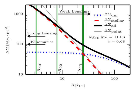
Figure 1: Predicted $\Delta\Sigma$ profile for galaxies with $\log_{10}(M^{*})\sim 11.3$ and at $z\sim 0.68$. The blue dotted line represents $\Delta\Sigma_{{\rm dm}}$ assuming an NFW profile. The red dashed line represents $\Delta\Sigma_{{\rm stellar}}$ computed using a Hernquist mass model. The thin grey line shows $\Delta\Sigma_{{\rm stellar}}$ computed using the point source approximation (Equation 7). The black solid line denotes $\Delta\Sigma$ which is the sum of $\Delta\Sigma_{{\rm dm}}$ and $\Delta\Sigma_{{\rm stellar}}$. The green thin vertical line labelled “$R_{90}$” shows the mean radius encompassing $90$ per cent of the flux from lens galaxies. Another green thin vertical line labelled “$R_{50}$” shows the half light radius of lens galaxies. The green thick vertical line shows the equality radius $R_{\rm eq}$. The purpose of this paper is to predict the S/N of weak lensing measurements on radial scales smaller than $R_{\rm eq}$.

2.2 Stellar-to-Halo Mass Relation

To estimate $M_{200{\rm b}}$ from $M_{*}$ for each lens galaxy, we adopt the stellar-to-halo mass relation (SHMR) from Leauthaud et al. (2012) (hereafter L12). In their study, L12 assume a lognormal distribution for the central galaxy conditional stellar mass function $P(M_{*}|M_{200{\rm b}})$. For central galaxies that reside in halos of mass $M_{200{\rm b}}$, the average of their logarithmic stellar mass, $f_{\rm SHMR}(M_{200{\rm b}})$, satisfies the following equation:

$$\log_{10}\left(f_{{\rm SHMR}}^{-1}(M_{*})\right)=\log_{10}\left(M_{200{\rm b}}\right)$$ (8)

$$=\log_{10}\left(M_{1}\right)+\beta\log_{10}\left(\frac{M_{*}}{M_{*,0}}\right)+\frac{\left(M_{*}/M_{*,0}\right)^{\delta}}{1+\left(M_{*}/M_{*,0}\right)^{-\gamma}}-\frac{1}{2}\,.$$

This functional form with parameters $M_{1}$, $M_{*,0}$, $\beta$, $\delta$, and $\gamma$ is motivated from Behroozi et al. (2010). We refer the reader to Leauthaud et al. (2011) and Behroozi et al. (2010) for the definitions of these parameters, notations, and how these parameters control the shape of SHMR.

L12 fit this model to the abundances of galaxies, their clustering, and the weak lensing signal from the COSMOS field in three redshift bins ($z\in[0.22,0.48]$, $[0.48,0.74]$, $[0.74,1.00]$). Their results suggest a very weak evolution of the global SHMR from $z=0.2$ to $z=1$, especially for low stellar mass galaxies with $M_{*}\lesssim 2\times 10^{10}$ ${\rm M_{\odot}}$. We use the SHMR parameters from L12 in each redshift bin.

Note that this SHMR is only valid for central galaxies. According to the modelling results from L12, about 20 per cent of galaxies in the COSMOS field are expected to be satellites. For our predictions, however, we neglect satellite galaxies and make the simplifying assumption that all lens galaxies are centrals.

The average halo mass of galaxies of a given stellar mass can be computed using $P(M_{200{\rm b}}|M_{*})$, which is related to $P(M_{*}|M_{200{\rm b}})$ via Bayes’ theorem

$$P(M_{200{\rm b}}|M_{*}) = \frac{P(M_{*}|M_{200{\rm b}})P(M_{200{\rm b}})}{P(M_{*})}$$ (9)

$$\propto P(M_{*}|M_{200{\rm b}})n(M_{200{\rm b}})\,,$$

where $n(M_{200{\rm b}})$ represents the halo mass function. For this analysis, we will use the Tinker et al. (2008) halo mass function. We calculate the average halo mass of galaxies within a given stellar mass bin $[M_{1},M_{2}]$ as:

$$\langle M_{200{\rm b}}\rangle_{[M_{1},M_{2}]}=\frac{\int_{M_{1}}^{M_{2}}dM_{*}\int_{0}^{\infty}M_{200{\rm b}}P(M_{200{\rm b}}|M_{*})dM_{200{\rm b}}}{\int_{M_{1}}^{M_{2}}dM_{*}\int_{0}^{\infty}P(M_{200{\rm b}}|M_{*})dM_{200{\rm b}}}\,.$$ (10)

The variation of $M_{200{\rm b}}$ as a function of lens stellar mass and redshift is shown in Fig. 2.

3 Small scale Weak lensing: Main effects

Our goal is to predict the expected S/N of weak lensing measurements within the equality radius $R_{\rm eq}$. A variety of different effects will impact the expected weak lensing signal at this radial scale. We list these effects below.

1. $R_{\rm eq}$ depends on the SHMR, the concentration-mass relation, and their evolution with redshift.

2. The angular diameter distance and its dependence on redshift determines the apparent area on the sky covered by a given $R_{\rm eq}$. For a fixed number of lens galaxies, a larger apparent area on the sky will correspond to a larger number of source galaxies and hence a higher S/N.

3. For a fixed survey area, the number of lens galaxies will increase with redshift because the survey covers a larger comoving volume.

4. The strength of the lensing signal (i.e, the shear) depends on the value of $\Sigma_{\rm crit}$ which depends on the redshift of the lens and the source. For a fixed source redshift, $z_{\rm s}$, the strength of the lensing signal peaks around $z_{\rm s}/2$.

5. The strength of the shear around lens galaxies will be large at $R_{\rm eq}$. We need to be mindful of the regime where lensing is no longer weak.

6. Magnification bias may alter the observed source density.

7. The amount of “real estate” between the radius at which the light from a lens becomes insignificant and $R_{\rm eq}$ depends on the sizes of lens galaxies.

8. Unbiased measurements of shapes are difficult for galaxies that are blended or that are close to other galaxies so proximity effects are important.

Some of these trends ((i)-(vi)) can be computed analytically. However (vii) and (viii) are non trivial. In particular, quantifying the effects of close pairs is especially difficult. For this reason, our predictions will be largely based on numbers drawn directly from a COSMOS weak lensing catalogue (see Section 4). Below, we discuss each of these effects in further detail with an emphasis on developing an intuition for how each effect drives our predicted S/N. We also clarify which components of our model are computed analytically and which components are drawn from real data.

3.1 Equality radius

As defined in Section 2.1, $R_{\rm eq}$ corresponds to the radius where the contributions of the dark matter component and the stellar component to $\Delta\Sigma$ are equal. The S/N of weak lensing measurement on such small scales depends on the number of background source galaxies that lie within a projected distance $r<R_{\rm eq}$. Hence, a larger value of $R_{\rm eq}$ should result in a larger S/N.

We compute $R_{\rm eq}$ by equating the right hand sides of Equations 6 and 7. Fig. 2 shows the variation of $R_{\rm eq}$ as a function of lens stellar mass and redshift. At a given redshift, $R_{\rm eq}$ increases with lens stellar mass. The increase in $R_{\rm eq}$ with stellar mass is in contrast to the $M_{*}/M_{200{\rm b}}-M_{200{\rm b}}$ relation, which shows a distinct peak at a preferred halo mass scale of $M_{\rm 200b}=10^{11.8}\mbox{${\rm M_{\odot}}$}$ (e.g., Behroozi et al. 2010; L12; Rodríguez-Puebla et al. 2013).

This trend can be easily understood in the following manner. In the inner regions of halos ($r\lesssim r_{{\rm s}}$), the profile function in Equation 6, $g(r/r_{\rm s})\approx 1$. Therefore, we obtain:

$$R_{\rm eq}\propto\left(\frac{M_{*}}{\left\langle M_{200{\rm b}}\right\rangle^{\frac{1}{3}}}\right)^{\frac{1}{2}}\overline{\rho}_{\rm b}^{-\frac{1}{3}}\,.$$ (11)

For a fixed redshift, $R_{\rm eq}$ is proportional to the first term in the above equation. We compute $\left\langle M_{200{\rm b}}\right\rangle$ from Equation 10, and find that the power law slope of the $\left\langle M_{200{\rm b}}\right\rangle-M_{*}$ relation is approximately unity at a stellar mass of about $\log_{10}(M_{*})=10.5$, which implies the approximate scaling $\log_{10}(R_{\rm eq})\propto 0.34\times\log_{10}(M_{*})$. This scaling is shown in Fig. 2 by a solid black line. It agrees with the increase of $R_{\rm eq}$ with stellar mass that we observe.

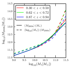
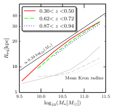
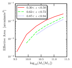
Figure 2: Left: variation of $M_{200{\rm b}}$ as a function of stellar mass and redshift based on SHMR. Coloured lines represent three different redshift bins for lens galaxies. Solid lines show $\left<M_{200{\rm b}}\right>$ whereas dashed line show $\left<\log_{10}(M_{*})\right>$. Differences between the solid and dashed lines are due to scatter in the SHMR relation. The green solid line corresponding to the redshift range ($0.62<z<0.72$) has been shifted horizontally by $0.03$ dex for presentation purposes. Middle: evolution of $R_{\rm eq}$ as a function of stellar mass and redshift. Coloured lines represent three different redshift bins for lens galaxies. Grey lines indicate the geometric mean of the semi-major and the semi-minor length of the Kron ellipses of lens galaxies. As a reference, the typical half light radius of lens galaxies at $z\sim 0.4$ is $R_{e}=2.4$ kpc for $M_{*}\approx 5.5\times 10^{9}\mbox{${\rm M_{\odot}}$}$ and $R_{e}=3.5$ kpc for $M_{*}\approx 1.3\times 10^{11}\mbox{${\rm M_{\odot}}$}$. Right: evolution of the effective area within $R_{\rm eq}$ as a function of stellar mass and redshift.

3.2 Effective Area within $R_{\rm eq}$

We will use the Kron ellipse (which roughly encompasses 90 per cent of the light) to define the spatial extent of lens galaxies (see Section 5.2). We define the effective area, $A_{\rm eff}$, as the angular area between the outskirts of lens galaxies (as traced by the Kron ellipse) and $R_{{\rm eq}}$ – this is a measure of how much “real estate” is available for weak lensing measurements at $R_{\rm eq}$. Fig. 2 shows how $A_{\rm eff}$ varies as a function of lens stellar mass and redshift. The redshift dependence of $A_{\rm eff}$ is driven by the angular diameter distance. A fixed value of $R_{{\rm eq}}$ corresponds to a larger effective area at lower redshifts. Fig. 2 shows that massive galaxies at low redshift have the largest effective area and by consequence, the largest number of source galaxies per lens within the equality radius.

3.3 Geometric Effects due to $\Sigma_{\rm crit}$

The strength of the lensing signal depends on the value of $\Sigma_{\rm crit}$, which depends on the redshifts of both lens and source galaxies. To gain an intuition for how $\Sigma_{\rm crit}$ drives S/N, let us consider a simple scenario in which we have a fixed number of lens galaxies $N_{\rm l}$ and a fixed high redshift source plane $z_{\rm s}$. The projected number density of sources is denoted as $n_{\rm s}$. The error on $\Delta\Sigma$ within a fixed physical aperture $R_{\rm ap}$ scales as $\sigma_{{}_{\Delta\Sigma}}\propto\Sigma_{{\rm crit}}\,N_{{\rm pairs}}^{-1/2}$ where $N_{\rm pairs}$ is the number of lens-source pairs. The number of lens-source pairs is simply:

$$N_{\rm pairs}=N_{\rm l}\times n_{\rm s}\times\pi R_{\rm ap}^{2}/D_{\rm ol}^{2}\,.$$ (12)

Putting these two together, the $D_{{\rm ol}}$ term cancels and the error on $\Delta\Sigma$ within a fixed physical aperture $R_{\rm ap}$ scales as:

$$\sigma_{{}_{\Delta\Sigma}}\propto\frac{D_{{\rm os}}}{D_{{\rm ls}}}.$$ (13)

For a fixed source redshift, a lower lens redshift results in a larger $D_{{\rm ls}}$, which corresponds to smaller error on $\Delta\Sigma$. Therefore, from a pure geometric point of view, the S/N for weak lensing measurements within a fixed aperture will increase at lower redshifts. This may seem in contrast to the common intuition that the S/N of weak lensing measurements peaks at about a redshift of $z_{\rm s}/2$. The reason for this difference is simply that Equation 13 assumes a fixed number of lens galaxies $N_{\rm l}$. In a weak lensing survey however, the number of lens galaxies per unit comoving line-of-sight distance will decrease towards low redshifts (causing $N_{\rm pairs}$ to also decrease).

In this paper, we are primarily interested in predictions for the S/N of weak lensing measurements for future weak lensing surveys. However, we note that Equation 13 implies that another strategy for maximizing the S/N of small scale weak lensing measurements is targeted observations of very low redshift massive galaxies (Gavazzi et al. 2007; Okabe et al. in prep.)

3.4 Amplitude of Shear on Small Scales

As we try to push towards small radial scales, the weak shear assumption, $|\gamma|<<1$, may no longer be valid. Most of the shear measurement pipelines are designed with cosmic shear studies in mind and are not necessarily well tested for large shear values. For example, the GRavitational lEnsing Accuracy Testing 3 (GREAT3) competition (Mandelbaum et al. 2014) only tested $\gamma$ up to values of $0.05$. In this section we calculate the amplitude of the shear signal at the equality radius to determine whether or not this still corresponds to a weak lensing regime.

At $r=R_{\rm eq}$, $\Delta\Sigma$ is simply:

$$\Delta\Sigma(R_{\rm eq})=2\times\frac{M_{*}}{\pi R_{\rm eq}^{2}}\,.$$ (14)

The left hand panel of Fig. 3 shows the dependence of $\Delta\Sigma(R_{\rm eq})$ on lens stellar mass and redshift. As discussed in Section 3.1, at fixed redshift, $R_{\rm eq}$ increases with stellar mass but with a shallow slope of $0.34$. Therefore, $\Delta\Sigma(R_{\rm eq})$ increases with stellar mass with a power law slope of $0.32$. Similarly, at a fixed stellar mass, $R_{\rm eq}$ decreases with redshift, leading to an increase in $\Delta\Sigma(R_{\rm eq})$ with redshift.

We now estimate the typical value of $\gamma$ at $r=R_{\rm eq}$. For simplicity, we assume that all source galaxies are located at a fixed redshift $z_{\rm s}=2$. The results are shown in the right hand panel of Fig. 3. The difference between the contour shapes in the left and the right panel are due to the dependence of $\Sigma_{\rm crit}$ on the lens redshift; for fixed $z_{\rm s}=2$, $\Sigma_{\rm crit}$ reaches a minimum at intermediate redshifts. We find that galaxies with $M_{*}>10^{11}\mbox{${\rm M_{\odot}}$}$, on average, will have shear values of order $0.05$–$0.01$ at $R_{\rm eq}$. Hence, these types of measurements will require a careful calibration of shear measurements up to values of about $0.1$. Biases in the shear measurement at such high values are currently being investigated by the ARCLETS collaboration.

Moreover, in this shear regime, the shapes of source galaxies are described by a combination of the shear and the convergence, called the reduced shear (Schneider & Seitz 1995). The interpretation of the small-scale weak lensing will require modelling of the reduced shear rather than the shear (that we investigate here). However, the difference between the two is expected to be relatively minor ($5$–$10$ per cent) on the radial scales and the halo mass scales considered in our work (e.g., Mandelbaum et al. 2006; Johnston et al. 2007; Leauthaud et al. 2010).

An important point to note here is that for our calculations, we are considering the value of the shear for the average halo at fixed lens stellar mass. The type of measurements that we are proposing here are not possible at the hearts of rich groups or clusters of galaxies at intermediate redshifts where the weak lensing approximation is clearly not valid. For massive galaxies, however, there is a large scatter in $M_{200{\rm b}}$ at fixed stellar mass (see e.g., More et al. 2011; L12). For example, at a fixed stellar mass of $\log_{10}(M_{*})=11$, there is a $0.46$ dex spread (a factor of $2.9$) in halo mass, and a $0.7$ dex spread (a factor of $5.0$) at $\log_{10}(M_{*})=10.5$. Our calculations are valid for the average halo at fixed stellar mass – not for galaxies in rich groups or clusters.

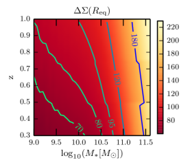
Figure 3: Left: variation of $\Delta\Sigma$ at $R_{\rm eq}$ as a function of lens stellar mass and redshift assuming source galaxies at $z_{\rm s}=2$. $\Delta\Sigma(R_{\rm eq})$ monotonically increases with stellar mass and redshift. Right: same as the left panel but for the shear $\gamma$. At fixed stellar mass, $\gamma$ reaches maximum values at $z\sim 0.6$.

3.5 Proximity Effects and Blends

To measure weak lensing signals, accurate and unbiased measurements of both shapes and photometric redshifts are critical. Such measurements are difficult when the angular separation between the lens and the source galaxy is small. In particular, the equality radius is merely a factor of 2-3 larger than the typical size of lens galaxies (as traced by the Kron ellipse, see Fig. 2). If a source galaxy is located too close to a lens, then the light from the lens galaxy may contaminate the photometry as well as the shape measurement of the source galaxy. Biases in shape measurements will directly translate into biases in the measured weak lensing signal. Biases in the photometry contribute indirectly via biases in photometric redshifts which are required to compute $\Sigma_{\rm crit}$. The magnitude of these proximity effects depend on the size distribution of lens galaxies but also on the size distribution of neighbouring galaxies that correlate with the lens sample. We will use existing COSMOS ACS data to estimate the magnitude of these effects. We will devote large parts of Section 5 in order to quantify the magnitude of proximity effects.

4 Data

As discussed in the previous section, among the various factors affecting the expected S/N of weak lensing measurements on small scales, the number of source galaxies lost due to proximity effects are the hardest to quantify analytically. It is primarily for this reason that we opt to use a real catalogue for the basis of our study instead of taking a semi-analytical approach such as the one explored by Dawson et al. (2014). We will use the COSMOS ACS catalogue (described in the subsequent section) as our primary catalogue with which to conduct this analysis. The COSMOS field is small which means that our choice represents a trade-off between area and high resolution imaging but, as we will show further on in this paper, proximity effects are the largest determining factor for our predictions which motivates our choice. We now describe the data products that we use in greater detail.

4.1 COSMOS Weak Lensing Catalogue

The COSMOS program has imaged the largest contiguous area (1.64 degrees²) with the Hubble Space Telescope (HST) using the Advanced Camera for Surveys (ACS) Wide Field Channel (WFC) (Scoville et al. 2007). The $5\sigma$ point-source limiting depth is $I_{\rm AB}=27.2\ \mathrm{mag}$ in a 0$\aas@@fstack{\prime\prime}$24 diameter aperture (Koekemoer et al. 2007) and the size of point spread function (hereafter PSF) is $0.12^{\prime\prime}$ (Leauthaud et al. 2007). This combination of depth and exquisite resolution over a moderately wide area motivates our choice to use this as our primary data set. The details of the COSMOS weak lensing catalogue have already been described in ample detail elsewhere (Massey et al. 2007; Leauthaud et al. 2007; Rhodes et al. 2007; L12). The COSMOS weak lensing catalogue contains $3.9\times 10^{5}$ galaxies with accurate shape measurements, which represents a number density of $66$ source galaxies per arcminute².

For shape measurements, the COSMOS weak lensing catalogue uses the RRG algorithm (Rhodes et al. 2000). The exact details of the shape measurement procedure are mostly un-important for this paper. We do however use information about when a shape measurement was possible with the expectation that the failure rate of galaxy shape measurement will increase for close lens-source pair configurations. The RRG COSMOS catalogue does not explicitly flag source galaxies that have close companions. However, galaxies may fail to converge on a shape measurement if the RRG algorithm fails to determine a centroid (which typically occurs for blends). This is in contrast to the lensfit algorithm, for example, which explicitly rejects galaxies in close pairs whose isophotes are overlap at two-sigma level of the pixel noise (Miller et al. 2007; Miller et al. 2013).

To select galaxies with precise shape measurements, we adopt the same four selection cuts as Leauthaud et al. (2007). In addition, we restrict ourselves to galaxies that are detected in the COSMOS Subaru catalogue (See Section 5.3) and with $0<\sigma_{\rm meas}<0.2$, where $\sigma_{\rm meas}$ represents the shape measurement error from Leauthaud et al. (2007). We also remove a small fraction of galaxies for which SourceExtractor (Bertin & Arnouts 1996) failed to measure the ${\rm KRON\_RADIUS}$ (see Section 5.2 for the definition of this parameter). These additional cuts remove $29$ per cent of galaxies from the COSMOS weak lensing catalogue, leaving $2.7\times 10^{5}$ galaxies ($45$ galaxies per arcminute²) with shape measurements and which are detected by the COSMOS Subaru observations.

4.2 COSMOS Photo-z Catalogue

Photometric redshifts (hereafter, “photo-zs”) are necessary in order to separate foreground and background galaxies. Ideally, our photo-zs would be determined from multi-band imaging matched in both resolution and depth to the COSMOS F814W imaging. However, the COSMOS photo-zs are measured from ground-based imaging with a PSF that is larger by about a factor of $10$ compared to the ACS data. In Section 5, we study how this photo-z matching affects our predictions.

For this paper, we use the COSMOS photo-z catalogue version 1.8 presented in Ilbert et al. (2009). These photo-zs have been derived using a $\chi^{2}$ template fitting method using over 30 bands of multi-wavelength data from UV, visible near-IR to mid-IR, and also have been calibrated with large spectroscopic samples from VLT-VIMOS (Lilly et al. 2007) and Keck-DEIMOS.

4.3 Stellar Mass Estimates

Stellar mass estimates are required in order to predict $\Delta\Sigma$. We use the same stellar mass estimates as L12 and refer the reader to L12 and Bundy et al. (2010) for further details.

Stellar mass estimates are based on PSF-matched 3$\aas@@fstack{\prime\prime}$0 diameter aperture photometry from the ground-based COSMOS catalogue (filters $u^{*},B_{J},V_{J},g^{+},r^{+},i^{+},z^{+},K_{s}$) (Capak et al. 2007; Ilbert et al. 2009; McCracken et al. 2010). The depth in all bands reaches at least 25th magnitude (AB) except for the $K_{s}$-band, which is limited to $K_{s}<24\,[\mathrm{mag}]$. Stellar masses are derived using the Bayesian code described in Bundy et al. (2006), which uses Bruzual & Charlot (2003) population synthesis code and assume a Chabrier IMF (Chabrier 2003) and a Charlot & Fall (2000) dust model. The stellar mass completeness is defined from magnitude limits $K_{s}<24\,[\mathrm{mag}]$ and $I_{{\rm 814W}}<25\,[\mathrm{mag}]$. For the redshift range that we are interested in here ($0.2\leq z\leq 1.0$), the stellar mass completeness ranges from $M_{*}=10^{8.16}$${\rm M_{\odot}}$ to $10^{9.98}$${\rm M_{\odot}}$.

5 Method

Here we describe the method that we use to compute the predicted S/N for $\Delta\Sigma(r<R_{\rm eq})$ for weak lensing data sets with COSMOS like quality. For a given set of foreground lens galaxies, the main ingredients necessary to make this prediction are the number of lens galaxies, the number of background galaxies with shape measurements as a function of distance, the shape noise for these background galaxies, and the redshift distribution of source galaxies. We describe how we extract these quantities from the COSMOS ACS catalogue.

5.1 Lens and Source Samples

There is some arbitrariness involved in the definition of the foreground lens sample used to perform a S/N investigation. The predicted value of the S/N depends on the number of galaxies in the lens sample, which depends on the choice of the binning scheme. For example, equal-sized redshift bins will provide a larger volume for higher redshift bins, which results in a larger number of galaxies in the higher redshift bins. In our work, we opt to divide our galaxies into $7$ equal comoving volume bins in redshift and $6$ logarithmically spaced stellar mass bins. In each redshift bin, we only consider bins that are complete in stellar mass (Section 4.3; L12). The characteristics of our lens samples are provided in Table 5.1.

Redshift	$\log_{10}M_{*}[{\rm M_{\odot}}]$
	$[$ 9.37 , 9.74 $]$	$[$ 9.74 , 10.11 $]$	$[$ 10.11 , 10.49 $]$	$[$ 10.49 , 10.86 $]$	$[$ 10.86 , 11.23 $]$	$[$ 11.23 , 11.60 $]$
$[$ 0.30 , 0.50 $]$	2477	2000	1690	1404	731	162
$[$ 0.50 , 0.62 $]$	1688	1185	1110	878	494	113
$[$ 0.62 , 0.72 $]$	$\times$	1476	1209	1144	750	212
$[$ 0.72 , 0.80 $]$	$\times$	1669	888	767	479	137
$[$ 0.80 , 0.87 $]$	$\times$	$\times$	1436	1458	943	266
$[$ 0.87 , 0.94 $]$	$\times$	$\times$	1107	993	622	173
$[$ 0.94 , 1.00 $]$	$\times$	$\times$	1185	1058	737	241
Mean number	2007.8	1526.4	1188.6	1049.9	645.9	171.9

Table 1: Number of lens galaxies from our COSMOS catalogue in bins of stellar mass and redshift. Bins that are incomplete in terms of stellar mass are shown as $\times$. The numbers in the bottom row are the mean values after the correction of sample variance described in Section 5.1.

Despite our choice of redshift bins with equal comoving volumes, the number of lens galaxies within each stellar mass bin fluctuates due to sample variance. We would like to minimize the effects of such variations on the calculated S/N. We make the assumption that the total stellar mass function of galaxies does not strongly evolve at $z<1$ (motivated by Bundy et al. 2010; Ilbert et al. 2010; L12; Moustakas et al. 2013). We fit a constant to the number of galaxies in each stellar mass bin, assuming Poisson statistics. The value of these constants are provided in Table 5.1 as “mean number”. We use this mean number in order to generate our predictions.

As our input catalogue for source galaxies, we use the COSMOS ACS weak lensing catalogue. As described in Section 4.1, we restrict ourselves to source galaxies that pass a combination of three quality cuts as well as four quality cuts described in Leauthaud et al. (2007). These galaxies form our source catalogue.

5.2 Impact of Proximity Effects on the Overall Source Density

In this section we explore how cuts based on proximity effects impact the overall source density. These estimates are of general interest for all weak lensing studies including efforts to measure cosmic shear for example.

Galaxies in close pairs may have biased shear estimates, but the exact level of such bias or how it varies as a function of the distance between close pairs, remains poorly understood. As a result, most current weak lensing pipelines do not necessarily have a well justified criterion to determine which galaxies have shapes that may be biased because of neighbouring galaxies. For example, the ACS lensing catalogue that we use in this paper makes no stringent cuts to remove source galaxies in close-pair configurations, even though these galaxies may have biased shear estimates. On the other hand, Miller et al. (2013) take a more conservative approach while constructing the CFHTLS weak lensing catalogue (see Section 4.1). However, both of these choices remain subjective and do not study the amount of shear bias in close pairs. Quantitative investigation of shear bias is a topic of active research, but is beyond the scope of this paper. Instead, we use a simple and easily reproducible criterion for identifying close pairs and we explore how the predicted S/N for small-scale lensing measurements varies for source galaxy selections that are more or less conservative.

Our scheme to identify close pairs of galaxies is based on the Kron parameters from SourceExtractor (Bertin & Arnouts 1996) (hereafter SExtractor), which generalizes the luminosity-weighted radius of Kron (1980) to elliptical apertures. Our choice is motivated by the fact that Kron parameters are often available in imaging catalogue, which makes our criterion easily reproducible. We note, however, that our procedure will not identify blends at a fixed isophotal level. While an isophotal definition of blends would have been preferable, it was not possible to calculate such a criterion given the catalogues available to us.

The Kron parameters consist of ${\rm A\_IMAGE}$, ${\rm B\_IMAGE}$, ${\rm KRON\_RADIUS}$, and ${\rm THETA\_WORLD}$. These parameters can be used to define a “Kron ellipse” for each galaxy that roughly encompasses $90$–$95$ per cent of the flux. For SExtractor, ${\rm KRON\_RADIUS}$ is computed by multiplying the first moment radius by a factor of $2.5$, then the major axis and the minor axis of the Kron ellipse are given by ${\rm A\_IMAGE\times KRON\_RADIUS}$ and ${\rm B\_IMAGE\times KRON\_RADIUS}$ respectively. The position angle of the Kron ellipse, ${\rm THETA\_WORLD}$, is measured between the right ascension and the direction of the semi-major axis.

We place Kron ellipses around all galaxies and identify galaxies with overlapping Kron ellipses. Our baseline predictions reject all source galaxies with overlapping Kron ellipses. In order to make this rejection criterion more or less conservative, we simply increase or decrease the size of the ellipse by multiplying the major and minor axis by a constant factor $f$. This procedure is illustrated in Fig. 4. The subsample of galaxies rejected by our criterion, when the multiplicative factor is $f$, will be denoted by $\sc{R}_{f}$. Those galaxies which are rejected when $f=f_{2}$ but not rejected when $f=f_{1}<f_{2}$, will be denoted by $\sc{R}_{[f_{1},f_{2}]}$. We use $f=1.0$ for our fiducial set of predictions and we explore how our predictions vary for different values of $f$. Table 5.1 shows the number and fraction of source galaxies that are rejected for various values of $f$.

Table 5.1 shows that the overall source density is very sensitive to proximity cuts. Rejecting all source galaxies that have a Kron ellipse that overlaps with a neighbouring galaxy leads to a $20$ per cent decrease in the overall source density. Adopting more conservative values of $f=1.2$ will lead to a $30$ per cent decrease in the overall source density. Understanding how neighbouring galaxies impact shear bias and which source galaxies need to be rejected is clearly of importance for all weak lensing studies, not just the particular science application discussed in this paper.

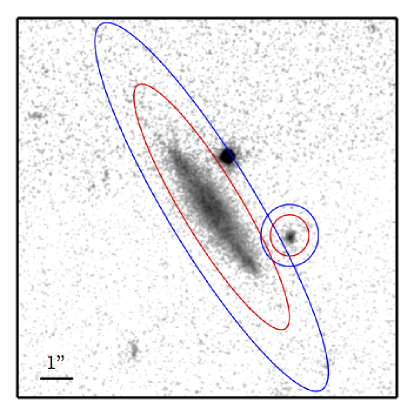
Figure 4: Two neighbouring galaxies with Kron ellipses overlaid. For the blue ellipses, the Kron ellipse has been scaled by a factor of $f=1.2$. For the red ellipses, the Kron ellipse has been scaled by a factor of $f=0.8$. These galaxies are rejected from our source catalogue when $f=1.2$ but are not rejected when $f=0.8$. The bright compact object is a star and does not belong in the source catalogue.

Table 2: The number and fraction of galaxies identified as close pairs in the source catalogue for different values of $f$. Our default scheme is $f=1$. In this case, $22.6$ per cent of galaxies are rejected from the overall source catalogue.

Fig. 5 shows an example of source galaxies selected by our method. In this figure, we show small cutout images around three massive lens galaxies at $z\sim 0.25$. Red ellipses indicate galaxies that have overlapping Kron ellipses. To predict the S/N of $\Delta\Sigma$ measurements within $R_{\rm eq}$, we only use source galaxies with green ellipses.

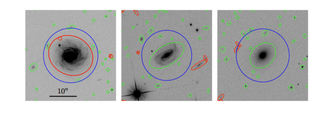
Figure 5: The three large galaxies at the centre of each postage stamp are examples of lens galaxies from the COSMOS survey at $z\sim 0.25$ and with $\log_{10}M_{*}[{\rm M_{\odot}}]\sim 11.1$. Green ellipses show Kron ellipses (here we use $f=1$). Blue circles show $R_{\rm eq}$. Galaxies with overlapping Kron ellipses are identified by red ellipses – these are rejected from our source catalogue. No circles or ellipses are drawn for stars.

5.3 Impact of Ground-Based Photometric Redshifts on Source Counts

In addition to shape measurements, weak lensing also requires photometric redshifts. The assignment of photometric redshifts to galaxies in close-pair configurations is non-trivial. Photometric redshifts are often derived from ground based imaging. For example, both Euclid (Laureijs et al. 2011) and WFIRST (Spergel et al. 2013) will need to complement their space-based imaging with ground based photometry. Because ground based imaging typically has a PSF of about one arcsecond, it may be difficult to derive accurate photometry for source galaxies at $R_{\rm eq}$.

We use the COSMOS photo-z catalogue to quantify how many source galaxies we lose due to this additional photometric redshift requirement. The detection of sources in this catalogue was carried out on a combined CFHT $i^{*}$ and Subaru $i^{+}$ image (with the original PSF of 0$\aas@@fstack{\prime\prime}$95) (Capak et al. 2007). Galaxy colours were measured with a 3$\aas@@fstack{\prime\prime}$0 aperture after PSF homogenization.

We now investigate the conditions under which shape and photometric redshift measurements fail in the COSMOS catalogues. Let us consider a galaxy A with a close-by companion galaxy B. We would like to know when shape and photo-z measurements typically fail for galaxy A as a function of the distance from B and as a function of the brightness ratio between galaxies A and B. To answer this question, we bin all of the galaxies in our ACS catalogue by magnitude and refer to it as our “primary” sample. For every galaxy in this sample, we identify all its neighbours in the entire ACS catalogue. We use a criteria based on Kron ellipses in order to scale distances between the primary and its neighbours. Pairs of primary-neighbour galaxies whose Kron ellipses overlap when their major and minor axes are scaled by a factor $f_{1}<f<f_{2}$, are labelled $\sc{R}_{[f_{1},f_{2}]}$. If there is more than one overlapping neighbour, we use the brightest one (this occurs in about $6$ to $10$ per cent of cases depending upon the value of $f$).

Fig. 6 shows how often shapes and photo-zs are measured for primary galaxies as a function of the distance and magnitude difference with the brightest neighbour. The two columns correspond to different primary samples (the fainter primary sample is on the right). The top row corresponds to galaxies in close pairs where the separations are small ($R_{[0.5,0.8]}$). We investigate close-pair galaxies with successively larger separations in the middle ($R_{[0.8,1.0]}$) and the bottom row ($R_{[1.0,1.3]}$). Fig. 6 shows that shape and photo-z measurements are more likely to fail for galaxies which have bright companions. Comparing the left and the right hand panels shows that this effect is more severe for faint galaxies. Comparing the different rows it is clear that the effect becomes smaller as we consider galaxies in close pairs but with larger separations.

In this test, we only consider when a galaxy has a photometric redshift measurement, but we do not evaluate whether or not photo-zs for galaxies with close by companions have a larger bias or a larger fraction of catastrophic errors. In addition, here we also only consider when a shape measurements has been possible, not whether or these shape measurements are biased. Obviously, these are aspects that need to be evaluated more critically in future work. Bearing these caveats in mind, Fig. 6 shows that shape measurements in the COSMOS catalogue are a more stringent requirement compared to photo-zs.

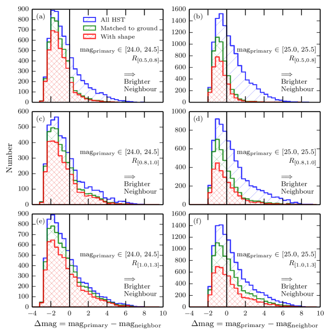
Figure 6: Number of galaxies in COSMOS as a function of the magnitude difference (mag(primary galaxy) - mag(neighbour galaxy)) between galaxies in close-pair configurations. Left panels: primary galaxies with magnitudes $\in[24.0,24.5]$. The distance to the closest neighbour increases from top to bottom ($R_{[0.5,0.8]}$ is a small separation and $R_{[1.0,1.3]}$ is a large separation). Blue histograms represents all galaxies in the COSMOS catalogue. Green histograms (“Matched to ground”) represent primary galaxies that have a photometric redshift measurement. Red histograms (“With shape”) represent primary galaxies that have a shape measurement and that pass our quality cuts as discussed in Section 4.1. Right panels: same as left panels but for primary galaxies with magnitudes $\in[25.0,25.5]$. This figure shows that both shape and photo-z measurements fail for source galaxies with bright companions. For example, panel d) shows that shape measurements fail for about 50 per cent of galaxies with magnitude $\in[25.0,25.5]$ and which have a close-by companion of equal magnitude ($\Delta mag=0$). This failure rate increases sharply for brighter companions ($\Delta mag>0$). Panel e) however shows that at mag$\in[24.0,24.5]$ and for $1.0<f<1.3$, most galaxies have both shape and photo-z measurements. A key point to note from this figure is that the red histograms are typically lower than the green: shape measurements in the COSMOS catalogue are a more stringent requirement compared to photo-zs.

5.4 Proximity Effects in the Number of Source Galaxies as a Function of Transverse Distance from Lenses

We investigate how blending affects the number of lens-source pairs as a function of transverse separation, $r$. The upper panels of Fig. 7 show the cumulative number of observed lens-source pairs, $N_{\rm pairs}(<r)$, in two different stellar mass bins and at one fixed redshift bin. Symbols with different colours correspond to all HST detected galaxies, those with photometric redshifts, and those that pass our source galaxy cuts. Note, however, that we have not yet imposed any proximity cuts on the source catalogue – galaxies with overlapping Kron ellipses are still included at this stage. For all samples in this figure, we also impose a magnitude cut at $i<26$. Note that we also do not yet impose a photo-z cut to separate foreground and background objects – we simply consider all pairs along the line-of-sight.

Fig. 7 shows that the overall number of lens-source pairs at large separations ($\sim 40$ kpc) decreases as we consider higher mass lens galaxies (indicated by the magenta vertical thin line). However, high mass lens galaxies have a larger number of lens-source pairs within $R_{\rm eq}$ (indicated by the magenta horizontal thin line). This is consistent with our expectations from Section 3.1: both $R_{\rm eq}$ and $A_{\rm effect}$ are larger for more massive galaxies. Because massive galaxies have a larger effective area where source galaxies can be found, they are more suited for detecting the small scale weak lensing signal.

The bottom panels of Fig. 7 show the ratio of $N_{\rm pairs}(<r)$ to the number of pairs expected from a simple power law extrapolation (with slope $-2$) of $N_{\rm pairs}(<r)$ from larger scales (thin grey line). These panels show that although a number of galaxies are detected at $r<R_{\rm eq}$, our photo-z and shape measurement requirements bring these numbers down significantly. Also, as discussed in the previous section, Fig. 7 shows that we lose more source galaxies due to the shape measurement requirement than the photo-z requirement. Note that all HST pairs in the higher mass lens bin outnumber the large-scale extrapolation on scales $\sim 20\mathrm{kpc}$. This bump feature indicates that galaxies are clustered with lens samples along the line-of-sight. These galaxies can be misinterpreted as source galaxies in our S/N predictions due to the photo-z errors. In Section 6.2, we will discuss such potential confusion in source selection due to correlated galaxies.

In addition to these effects, galaxies will also be rejected from our source catalogue due to the proximity cuts defined in Section 5.2. We are interested to know if source galaxies are flagged as overlaps at $R_{\rm eq}$ because they overlap with the lens galaxy under consideration, or because they overlap with non-lens galaxies.. Fig. 8 quantifies the relative importance of the two effects. For low stellar mass galaxies, we find that the majority of source galaxies lost within $R_{\rm eq}$ are due to overlap with the lens galaxy itself. At higher stellar masses we find that only $\sim$30 per cent of the source galaxies flagged as overlaps are colliding with the primary lens sample. The remaining $\sim$70 per cent overlap with either nearby galaxies that correlate with the primary lens sample, or with galaxies that are spatially uncorrelated with the lens sample. Again in this figure, we consider all pairs along the line-of-sight without the photo-z cut.

Finally, to select only source galaxies located at higher redshifts than lens galaxies, we impose a photo-z cut $z_{\rm s}>z_{\rm l,max}$ where $z_{\rm l,max}$ represents the upper redshift limit of the lens bin under consideration $[z_{\rm l,min},z_{\rm l,max}]$. The combination of the photo-z cut, the shape measurement cut and the proximity cut results in the cumulative number distribution of lens-source pairs shown in Fig. 9. Symbols with different colours correspond to source galaxies that pass only photo-z cut and shape measurement cut (in red), those that pass also proximity cut with $f=1$ (in green), and those that pass also proximity cut with $=1.3$ (in blue). In the fiducial case ($f=1$), the fraction of source galaxies within $R_{\rm eq}$ that pass the photo-z cut, but are rejected due to a combination of the shape measurement cut and the proximity cut is over $80$ per cent. We will use the $N_{\rm pairs}(<R_{\rm eq})$ in order to estimate the error on the weak lensing measurement within $R_{\rm eq}$ for every stellar mass and redshift bin in our sample. We compute the weak lensing signal at the average separation between the lens-source pairs using Equations 6 and 7.

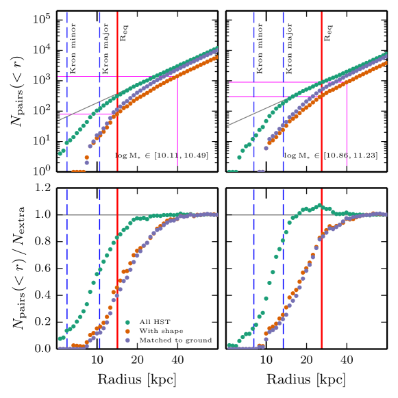
Figure 7: Upper panels: cumulative number of lens-source pairs, $N_{\rm pairs}(<r)$, as a function of the transverse distance from lens galaxies at $z\in\left[0.62,0.72\right]$. Left panels correspond to lens galaxies with $\log_{10}M_{*}\in\left[10.11,10.49\right]$. Right panels correspond to lens galaxies with $\left[10.86,11.23\right]$. Blue dashed vertical lines indicate the average semi-major and semi-minor axis of Kron ellipses for lens galaxies. The thick red vertical line denotes $R_{\rm eq}$. Green dots indicate all galaxies from the COSMOS weak lensing catalogue with $i<26$. Red dots represent galaxies with shape measurements. Blue dots represent galaxies that are matched to the ground-based photo-z catalogue. Note that no photo-z cuts have been applied to limit source galaxies to background galaxies (these cuts will be applied in Fig. 9. Magenta vertical thin line shows the location of $r=40$ kpc, and magenta horizontal thin lines respectively show $N_{\rm pairs}(<40\mathrm{kcp})$ and $N_{\rm pairs}(<R_{\rm eq})$. Lower panels: $N_{\rm pairs}(<r)$ divided by the expected number based on an extrapolation from larger scales ($N_{\rm extra}$). The lower panels show that proximity effects starts to influence the source galaxy counts at $r\sim 40$ kpc (roughly $1$ to $5$ times larger than $R_{\rm eq}$) and photo-z matching and shape cuts reduce $N_{\rm pairs}(<r)$ by 20-60 per cent at $r<R_{\rm eq}$. Note that we have not applied any cuts to removed overlapping galaxies, this will further reduce $N_{\rm pairs}(<r)$.

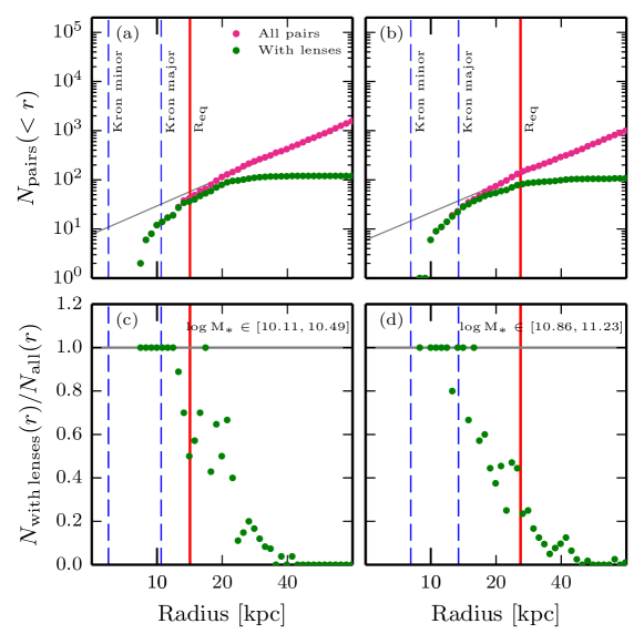
Figure 8: Similar to Fig. 7 but here we only show galaxies which have a Kron ellipse that overlaps with a neighbouring galaxy ($f=1$). Upper panels: cumulative number of galaxies identified as close pairs as a function of the transverse distance from lens galaxies. We distinguish overlaps that occur between a source and a lens from the sample under consideration from overlaps that occur between a source and some other non-lens galaxy. Magenta dots indicate the cumulative number of all source galaxies that are flagged are overlaps. Green dots represent source galaxies that have a Kron ellipse that overlaps with the Kron ellipse of a lens galaxy. The overall amplitude of $N_{\rm pairs}(<r)$ on larger radial scales is dominated by overlap between source galaxies that are spatially uncorrelated with the lens sample. On the other hand, the radial dependence of $N_{\rm pairs}(<r)$ on smaller radial scales is mainly driven by overlap with the primary lens sample and with galaxies that are correlated with the lens galaxies. Note that no photo-z cuts have been applied to limit source galaxies to background galaxies (these cuts will be applied in Fig. 9). Lower panels: fraction of source galaxies flagged as overlaps and for which the overlap occurs with a lens galaxy from the sample under consideration. Panel c) shows that for the lower stellar mass bins, overlaps mainly occur at $R_{\rm eq}$ because source galaxies tend to overlap with galaxies from the primary lens sample. Panel d) on the other hand, shows that for the higher stellar mass bins, only $\sim$30 per cent of the source galaxies flagged as overlaps are colliding with the primary lens sample. The remaining $\sim$70 per cent overlap with either galaxies that are spatially correlated with the lens sample or with galaxies that are uncorrelated with the lens galaxies.

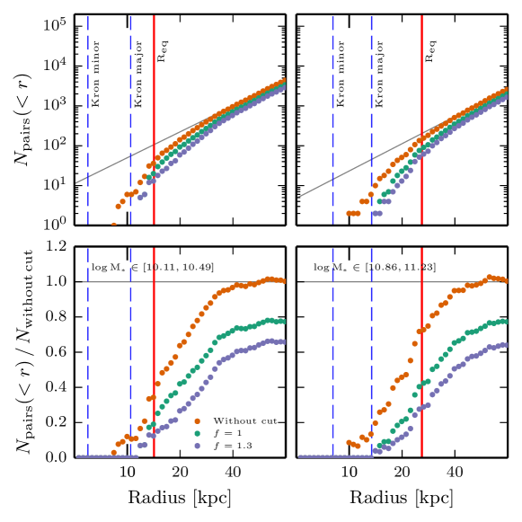
Figure 9: Upper panels: similar to Fig. 7 but here we show only source galaxies that pass also the photo-z cut. Red dots represent all source galaxies with both shape and photo-z measurements. Green dots represent only source galaxies that pass our proximity cut with $f=1$. Similarly, blue dots represent only source galaxies that pass our proximity cut with $f=1.3$. Lower panels: $N_{\rm pairs}(<r)$ divided by $N_{\rm without\,cut}$ where $N_{\rm without\,cut}$ is the extrapolation from larger scales of the source counts without any proximity cuts (red points). With $f=1$, the overall source density is reduced by 20 per cent. With $f=1.3$, the overall source density is reduced by 30 per cent (also see Table 5.1). Proximity effects start to impact $N_{\rm pairs}(<r)$ at $40$ kpc. At the equality radius, the source density is reduced by $60$–$80$ per cent for $f=1$.

5.5 $N_{\rm pairs}(<R_{\rm eq})$ : Number of Lens-Source Pairs Within the Equality Radius

We compute the total number of source galaxies that pass the photo-z cut, the shape measurement cut, the proximity cut, and which have $r<R_{\rm eq}$ for each of our lens bins. The values for $N_{\rm pairs}(<R_{\rm eq})$ for $f=1$ are given in Table 5.1. As can be seen from Table 5.1, the overall number of lens-source pairs for any given bin is small, only of order $\sim 100$. The difference between Tables 5.1 and 5.1 agrees with the results our conclusions from Section 5.4 – low-mass lens galaxies have almost no source galaxies within $R_{\rm eq}$ due to the small size of $R_{\rm eq}$.

Table 3: The number of lens-source pairs for $r<R_{\rm eq}$ for each of our lens bins. Source galaxies which have Kron ellipses that overlap with any nearby galaxy ($f$=1) are rejected from the source catalogue before computing these numbers. The photo-z cut to seperate background and foreground source galaxies has also been applied before compute these numbers.

5.6 Error on $\Delta\Sigma$ and Signal to Noise Ratio

Following Leauthaud et al. (2007), the error on the shear for each source galaxy is estimated as a combination of intrinsic shape noise ($\sigma_{{\rm int}}=0.27$) and shape measurement error:

$$\sigma_{\tilde{\gamma}}^{2}=\sigma_{{\rm int}}^{2}+\sigma_{{\rm meas}}^{2}\,.$$ (15)

The optimal weight for each source galaxy is given by

$$w_{i}=\frac{1}{\left(\Sigma_{{\rm crit},i}\,\sigma_{\tilde{\gamma},i}\right)^{2}}\,,$$ (16)

and the estimated error on $\Delta\Sigma$ in the COSMOS survey is given by

$$\sigma^{\rm COSMOS}_{{}_{\Delta\Sigma}}=\left[\sum\limits_{i}^{N_{\rm pairs}(<R_{\rm eq})}w_{i}\right]^{-1/2}\,,$$ (17)

The sum runs over all lens-source pairs with $r<R_{\rm eq}$ in a given stellar mass and redshift bin.

To scale our error estimate to survey areas larger than COSMOS, we assume that the distribution of source galaxy redshift and shape measurement errors in COSMOS are representative and we simply scale the estimated errors according to

$$\sigma^{\rm survey}_{{}_{\Delta\Sigma}}=\sigma^{\rm COSMOS}_{{}_{\Delta\Sigma}}\sqrt{\frac{A_{\rm COSMOS}}{A_{\rm survey}}}\,.$$ (18)

where $A_{\rm COSMOS}=1.64$ deg². Finally, combining $\Delta\Sigma$ and $\sigma_{\Delta\Sigma}$ (Equations 3 and 17), the predicted S/N in each stellar mass and redshift bin for COSMOS is simply

$${\rm S/N}=\frac{\Delta\Sigma}{\sigma_{\Delta\Sigma}}\,.$$ (19)

5.7 Predictions for COSMOS

Using Equations 17 and 19, we compute the expected S/N for one weak lensing data point at $r<R_{\rm eq}$ in the COSMOS ACS catalogue. The results are shown in Fig. 10. We find that the S/N for this type of measurement is maximized for massive galaxies at low redshifts, in agreement with our intuitive expectation from Section 3.4. We also show the effects of making more or less conservative source galaxy selections by varying our $f$ factor. A larger value of $f$ means that we reject more source galaxies in close-pair configurations. We find that varying $f$ between 0.8 and 1.3 only has a relatively minor impact on the predicted S/N. This implies that a more conservative selection of sources galaxies does not necessarily have a strong impact on the S/N.

6 Predictions for Euclid and WFIRST

In this section, we present our predictions for the S/N for small scale weak lensing measurements from future space-based surveys Euclid and WFIRST.

6.1 Next Generation Weak Lensing Space Based Surveys

Euclid is a space mission under development for an expected launch in 2020 (Laureijs et al. 2011). Euclid consists of a $1.2$ m Korsch telescope and two instruments, the VIS (visible imager) and NISP (Near Infrared Spectrometer and Photometer) and is designed to study the properties of dark energy and dark matter and to search for evidence of modified gravity by using weak gravitational lensing and galaxy clustering. Euclid will perform a 6 year imaging and spectroscopic survey over the lowest background $15000$ deg² of the extragalactic sky. Visible imaging in a single wide riz filter will provide shapes for about $1.6$ billion galaxies; near infrared imaging in $Y,J,H$ bands combined with ground-based photometry will enable high precision photometric redshifts for source galaxies. Euclid will have a $\sim$0.2 arcsecond PSF and will measure galaxy shapes with a source density of $\sim$30 galaxies per arcmin².

The Wide Field Infrared Survey Telescope (WFIRST) is a NASA mission under study for possible launch in $\sim 2024$ (Spergel et al. 2013). WFIRST consists of $2.4$m telescope a Wide Field Imager with 18 4k$\times$4k near infrared (NIR) detectors with $0.1$ arcsecond pixels, an integral field unit (IFU) spectrograph, and an exoplanet coronagraph. WFIRST is designed to perform NIR surveys for a wide range of astrophysics goals, including weak lensing. WFIRST’s weak lensing survey will cover $2400$ deg² and make galaxy shape measurements in $3$ NIR bands of about $500$ million galaxies over the course of two years in WFIRST’s primary mission of 6 years. WFIRST will have a PSF of 0.1 arcseconds (before pixellization) at 1 micron and about 0.2 arcseconds at 2 microns and will measure galaxies shapes with a source density of $\sim$54 galaxies per arcmin².

6.2 Predictions for one bin at $r<R_{\rm eq}$

To make our predictions for Euclid, we assume a source density of 30 galaxies per arcmin² over $15000$ deg². To mimic this source density, we simply apply a detection signal-to-noise cut on our COSMOS catalogue. After applying a signal-to-noise cut that yields 30 galaxies per arcmin², we rederive $N_{\rm pairs}^{EUCLID}(<r)$ for Euclid.

WFIRST is expected to achieve a source density of $\sim$54 galaxies per arcmin² over $2400$ deg². The COSMOS source density with reliable shape measurements and photo-zs (Section 4.1) is only of order $\sim$45 galaxies per arcmin², thus we cannot directly generate predictions for the expected WFIRST source density. Instead, for WFIRST, we will use 45 galaxies per arcmin². Our estimates for WFIRST will be conservative in this regard.

As mentioned earlier in Section 5.6, our predictions make several simplifying assumptions. First, we use the same shape noise as COSMOS (we do not attempt to adjust the measurement error component of the shape noise). Secondly, we use photometric redshifts from COSMOS, ignoring the fact for example, that WFIRST will detect galaxies in redder bands, and thus a somewhat higher redshifts. Finally, we also ignore the extra effects of smearing by a larger PSF ($\sim$ a factor of $1$–$2$ larger compared to COSMOS) on $N_{\rm pairs}(r)$, the number of source galaxies as a function of transverse separation. A more detailed study should account for such effects, but our goal here is simply to generate a first order prediction for the expected S/N.

We compute $N_{\rm pairs}^{EUCLID}(<r)$ for Euclid and use $N_{\rm pairs}^{COSMOS}(<r)$ for WFIRST. The expected S/N for one weak lensing data point at $r<R_{\rm eq}$ is then computed using Equations 18 and 19. The results are shown in Fig. 11. Similarly to Fig. 10, we observe that the S/N for both Euclid and WFIRST reaches its maximum for massive galaxies at lower redshifts. Fig. 11 indicates that Euclid and WFIRST may detect $\Delta\Sigma$ on very small radial scales with very high S/N greater than 20 for lens galaxies with $\log_{10}(M_{*})>10.4$. Note that this is lower mass than the mass probed by strong lensing, which is typically $\log_{10}(M_{*})>11.0$ (e.g., Auger et al. 2010b; Oguri et al. 2014; Sonnenfeld et al. 2014).

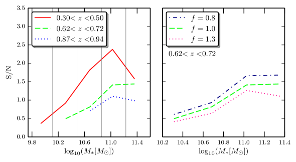
Figure 10: Predicted S/N for $\Delta\Sigma$ measured within $R_{\rm eq}$ as a function of lens stellar mass and redshift in the COSMOS field. Left: predicted S/N for three lens redshift bins assuming our fiducial close-pair cut with $f=1$. Grey vertical lines represent our lens stellar mass bins. Note that the S/N with $z\in[0.3,0.5]$ decreases rapidly at the highest stellar mass bin because the number of lens-source pairs decrease at high mass end (See Table 5.1). Right: expected S/N when we make more or less conservative cuts on source galaxies in close pair configurations (only the middle redshift bin is shown here). A larger value of $f$ corresponds to a more conservative selection of source galaxies. Varying $f$ between 0.8 and 1.3 only has a relatively minor impact on the predicted S/N.

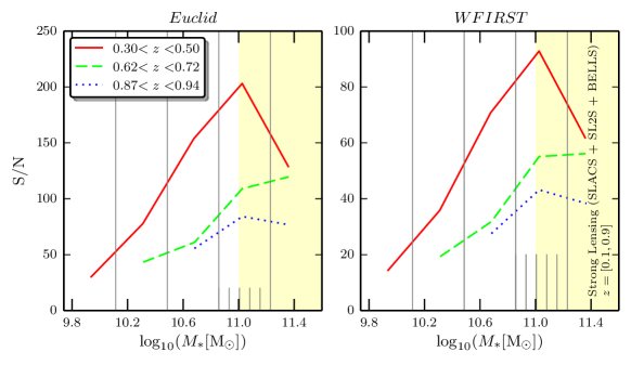
Figure 11: Similar to Fig. 10, but for future surveys – the left panel is for Euclid and the right panel is for WFIRST. Again, we assume our fiducial close-pair cut with $f=1$ and grey vertical lines indicate our lens stellar mass bins. Short grey thin lines represent the division of one the stellar mass bins into 5 smaller bins of width $0.074$ dex. Our prediction signal in Figs. 13 and 14 will adopt this finer binning scheme. Note that the S/N with $z\in[0.3,0.5]$ decreases rapidly in the highest stellar mass bin due to smaller number of lens-source pairs (also seen in Fig. 10). The yellow shaded region with $\log_{10}(M_{*})[\mbox{${\rm M_{\odot}}$}]\geq 11.0$ indicates the typical stellar mass range for strong lensing samples from the SLACS, SL2S, and BELLS surveys with $z\in[0.1,0.9]$. Although WFIRST will have a higher source density, its smaller area results in smaller S/N compared with Euclid.

Until now, all analyses presented in this section involve the photo-z cut, which uses best-fit photo-z on both lens and source samples. However, as we observed in Fig. 7, the confusion in source selection due to photo-z errors might be buried in our analyses even after the close-pair cut is applied (e.g., galaxies that are correlated with lens samples). To investigate such possibility, we employed several stringent photo-z cuts to separate lens and source galaxies and re-compute the predicted S/N. For example, to remove galaxies that are correlated with lens samples but have $z>z_{\rm l,max}$, we applied an additional buffer redshift to the maximum photo-z in each lens bin as

$$z_{\rm s}>z_{\rm l,max}+0.1(1+z_{\rm l,max})\,.$$ (20)

The buffer of $0.1$ is motivated by results from Ilbert et al. (2009), who report a one-sigma error on the best-fit photo-z of about $\sigma_{z}/(1+z)=0.07$ for objects with $i^{+}\sim 25.5$, which is more conservative than the expected errors in Euclid and WFIRST (see Laureijs et al. 2011 and Spergel et al. 2013 respectively). The resultant S/N is shown in Fig. 12. The predicted S/N decrease up to $10$ per cent at the higher mass end but the stringent cut (Equation 20) does not alter the overall trend – the S/N is maximized at massive galaxies at lower redshifts.

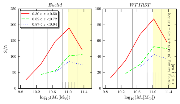
Figure 12: Similar to Fig. 11 but with a stringent photo-z cut applied (see Equation 20). Compared with Fig. 11, the S/N at the higher mass end decreases up to $10$ per cent but the overall dependence on the stellar mass and the redshift of lens galaxies does not change. Therefore, the confusion in source selection due to galaxies that are correlated with lens samples can be mitigated by such photo-z cuts. This may reduce S/N by a few per cent, but does not alter our main conclusion -– massive galaxies at lower redshifts yield higher S/N.

6.3 Predictions for radial bins

Figs. 10 and 11 show the expected overall S/N for one bin at $r<R_{\rm eq}$. We now consider the expected S/N in finer radial bins. Figs. 13 and 14 show the predicted errors on $\Delta\Sigma$ for lens galaxies with the mean stellar mass of $10^{11.03}$${\rm M_{\odot}}$ with the bin width of $0.074$ dex ($5$ times smaller than our bins in Table 5.1) at a mean redshift of $z=0.68$. The radial binning scheme is arbitrary – we opt to make $451$ bins with logarithmically equal width from $0.013$ to $419$ kpc. An NFW profile is assumed for the dark matter component and a Hernquist profile is assumed for the stellar component. This prediction uses source galaxies that pass all the quality cuts introduced in Section 4.1 including our fiducial close pair cut with $f=1.0$.

As a reference, in Figs. 13 and 14 we show how $\Delta\Sigma$ varies when the stellar mass of the lens sample varies by $\pm 0.2$ dex (a factor of $1.5$). As can be seen from these figures, both WFIRST and Euclid should be able to tightly constrain a combination of the inner dark matter slope and the total stellar mass of galaxies down to $\log(M_{*})>10.4$.

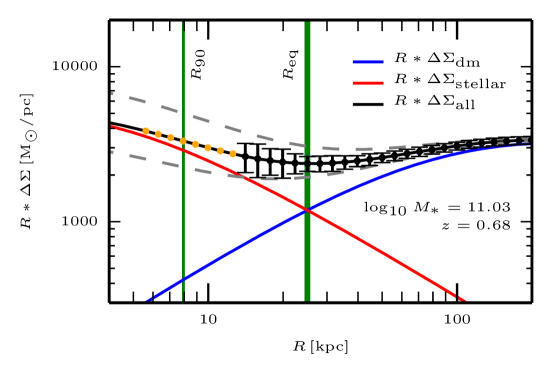
Figure 13: Predicted S/N on the $\Delta\Sigma(r)$ profile of lens galaxies with $\log_{10}(M*)=11$ for WFIRST. Note that the vertical scale is multiplied by $R$ to highlight the error bars. The dark matter profile ($\Delta\Sigma_{\rm dm}$) is shown by the blue line and the stellar component ($\Delta\Sigma_{{\rm stellar}}$) is shown by the red line. The black line represents the sum of $\Delta\Sigma_{\rm dm}$ and $\Delta\Sigma_{\rm stellar}$. The green thin vertical line indicates the radius that encompasses $90$ per cent of the flux of the lens galaxies. The green thick vertical line shows $R_{\rm eq}$. Grey dashed lines show $\Delta\Sigma$ when $M_{*}$ is varied by $\pm 0.2$ dex (roughly corresponding to the current uncertainty on the IMF). Yellow points indicate radial bins where there are no source galaxies in our COSMOS catalogue.

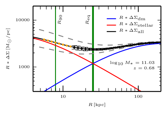
Figure 14: Same as Fig. 13 but for Euclid. Euclid will have a lower source density compared to WFIRST but will observe an area $6$ times larger ($15000$ deg² versus $2500$ deg²). This results in a factor of 2 in the expected S/N for Euclid compared to WFIRST. Note, however, that we have neglected other effects (e.g., the PSF size of EUCLID is twice as large as WFIRST) which will probably affect these predictions at a similar level.

7 Summary and Conclusions

Current constraints on dark matter density profiles from weak lensing are typically limited to radial scales greater than $r\sim 50$–$100$ kpc. Below this scale, there is a paucity of sources (background) galaxies due to poor image quality (“seeing”), complicating effects such as isophotal blending that inhibits shape measurements, and a lack of source galaxies simply due to the relatively small areas covered by current lensing surveys. Pushing weak lensing measurements down to smaller radial scales, however, would open up the exciting possibility of probing the very inner regions of galaxy/halo density profiles. Such measurements are currently only possible for strongly lensed galaxies which are rare, occur mainly for massive galaxies, and may also represent a biased sample. Weak lensing on these small scales would extend constraints to a much wider range of redshifts, stellar masses, and to an unbiased selection of galaxy types.

In this paper, we use a weak lensing catalogue from the COSMOS survey to investigate the expected S/N of stacked weak lensing measurements on radial scales of only a few tens of kpc. On these scales, in addition to dark matter, the weak lensing signal is sensitive to the baryonic mass of the host galaxy. Thus, future weak lensing measurements will offer the exciting possibility of directly measuring mass-to-light ratios and providing independent constraints on the Stellar Initial Mass Function (IMF) and on the interplay between baryons and dark matter.

We introduce the “Equality radius”, $R_{\rm eq}$, as the radius where the dark matter component and the stellar component contribute equally to the weak lensing observable, $\Delta\Sigma$. Using a stellar-to-halo mass relation that has been calibrated for COSMOS data, we compute the evolution of $R_{\rm eq}$ as a function of lens stellar mass and redshift. We show that $R_{\rm eq}$ is of order $7$ kpc for $M_{*}=10^{9.6}$${\rm M_{\odot}}$ and $34$ kpc for $M_{*}=10^{11.4}$${\rm M_{\odot}}$ at $z=0.4$. For lens galaxies with $M_{*}>10^{10.3}$${\rm M_{\odot}}$, this equality radius is about a factor of two larger than the size of the Kron ellipse which encompasses roughly $90$ per cent of the light. This leaves a very narrow window (width of order $10$ kpc) with which to measure weak lensing signals on scales where the stellar component dominates the lensing signal. The area of this window (per lens galaxy) $A_{\rm eff}$ varies between $2\times 10^{-4}$ arcminute² and $0.3$ arcminute². We show that $A_{\rm eff}$ is maximal for high mass galaxies at low redshifts due to the fact that a) $R_{\rm eq}$ is large for massive galaxies and b) a fixed value of $R_{\rm eq}$ in physical units corresponds to a larger angular size at low redshifts.

Using COSMOS, we calculate the number of lens-source pairs as a function of transverse separation $N_{\rm pairs}(r)$ down to $r=5$ kpc. We show that in the COSMOS catalogue, more galaxies in close-pair configurations are rejected because of cuts related to the quality of shape measurements rather than due to cuts related to the availability of a photo-z measurement. This test is simplistic in the sense that we only consider the availability of a shape or a photo-z measurement – not the quality of these measurements. This question obviously needs to be studied in greater detail, but this simple tests suggests that shape measurements rather than photo-z measurements may be the limiting factor for these types of studies.

We investigate how blending and proximity affect the source counts as a function of transverse distance from the lens sample. We show that within $R_{\rm eq}$, the number of source galaxies is reduced by $\sim 20$ per cent at $M_{*}=10^{11.0}$${\rm M_{\odot}}$ and by $60$ per cent at $M_{*}=10^{10.3}$${\rm M_{\odot}}$ due to blending. This sharp decrease in the number of source galaxies on small radial scales is due to the effects of masking/blending by foreground galaxies (Simet & Mandelbaum 2014). We quantify how often blends occurring at $R_{\rm eq}$ are due to the lens sample or to other (non lens) galaxies that are source galaxies and spatially correlated with the lens sample. At $R_{\rm eq}$ at $z=0.67$, we show that almost all blends occur with the lens sample with $M_{*}=10^{10.3}$${\rm M_{\odot}}$ whereas only about $30$ per cent blends occur with lens galaxies with $M_{*}=10^{11.0}$${\rm M_{\odot}}$.

Using a simple criterion based on the overlap between Kron ellipses, we study how $N_{\rm pairs}(r)$ varies with $f$. Over all the stellar mass range, larger $f$ rejects more source galaxies and results in lower S/N, which modifies the amplitude of S/N a factor less than $2$ from $f=0.8$ to $1.3$ and does not change the peak of S/N as a function of the stellar mass.

Finally, we use our COSMOS weak lensing catalogue to make a first prediction for the S/N for weak lensing measurements at $r<R_{\rm eq}$ for Euclid and WFIRST. Our predictions show that future experiments should have enough source galaxies on small scales to detect weak lensing down to a few tens of kpc with high S/N. Our predictions show that this idea is worth pursuing further - but make a number of simplifying assumptions that need to be investigated in further detail.

Our work has focused primarily on quantifying the effects on blends on the number of source galaxies at $r<R_{eq}$. In terms of raw numbers, our work shows that even after making a fairly conservative selection for our source galaxies, Euclid and WFIRST should still have a sufficient number of pairs on small scales to measure weak lensing with high S/N. This type of measurements however, will face a number of challenges which still need to be investigated. The main challenges that remain to be tackled will be understanding how to measure both shear and photometric redshifts in an unbiased fashion in close-pair configurations. In addition, further work is needed to test and calibrate shear measurements in this intermediate regime where the shear takes on values above 0.05. Also, here we have only considered stellar mass, but in addition the gas component may also be non-negligible especially at higher redshifts (Papastergis et al. 2012). Finally, but not least, understanding how to separate source galaxies from other galaxies spatially associated with lens galaxies and how to correct for boost factors (Mandelbaum et al. 2005) represent another challenge to be investigated in greater detail.

Acknowledgements

We are grateful to the referee for a careful reading of the manuscript and for providing thoughtful comments. We thank Robert Lupton for useful discussions during the preparation of this paper and Naoshi Sugiyama for practical advice during the data analysis. This work, AL, and SM are supported by World Premier International Research Center Initiative (WPI Initiative), MEXT, Japan. MINK acknowledges the financial support from N. Sugiyama (25287057) by Grants-in-Aid from the Ministry of Education, Culture, Sports, Science, and Technology of Japan. N. Okabe(26800097) is supported by Grants-in-Aid from the Ministry of Education, Culture, Sports, Science, and Technology of Japan. C. Laigle is supported by the ILP LABEX (under reference ANR-10-LABX-63 and ANR-11-IDEX-0004-02). J. Rhodes was supported by JPL, run under a contract for NASA by Caltech. TTT has been supported by the Grant-in-Aid for the Scientific Research Fund (23340046), for the Global COE Program Request for Fundamental Principles in the Universe: from Particles to the Solar System and the Cosmos, and for the JSPS Strategic Young Researcher Overseas Visits Program for Accelerating Brain Circulation, commissioned by the Ministry of Education, Culture, Sports, Science and Technology (MEXT) of Japan.

References

- Arraki et al. (2014) Arraki K. S., Klypin A., More S., Trujillo-Gomez S., 2014, MNRAS, 438, 1466
- Auger et al. (2010a) Auger M. W., Treu T., Gavazzi R., Bolton A. S., Koopmans L. V. E., Marshall P. J., 2010a, ApJ, 721, L163
- Auger et al. (2010b) Auger M. W., Treu T., Bolton A. S., Gavazzi R., Koopmans L. V. E., Marshall P. J., Moustakas L. A., Burles S., 2010b, ApJ, 724, 511
- Barnabè et al. (2013) Barnabè M., Spiniello C., Koopmans L. V. E., Trager S. C., Czoske O., Treu T., 2013, MNRAS, 436, 253
- Behroozi et al. (2010) Behroozi P. S., Conroy C., Wechsler R. H., 2010, ApJ, 717, 379
- Bertin & Arnouts (1996) Bertin E., Arnouts S., 1996, A&AS, 117, 393
- Blumenthal et al. (1986) Blumenthal G. R., Faber S. M., Flores R., Primack J. R., 1986, ApJ, 301, 27
- Bruzual & Charlot (2003) Bruzual G., Charlot S., 2003, MNRAS, 344, 1000
- Bundy et al. (2006) Bundy K., et al., 2006, ApJ, 651, 120
- Bundy et al. (2010) Bundy K., et al., 2010, ApJ, 719, 1969
- Capak et al. (2007) Capak P., et al., 2007, ApJS, 172, 99
- Cappellari et al. (2012) Cappellari M., et al., 2012, Nature, 484, 485
- Chabrier (2003) Chabrier G., 2003, PASP, 115, 763
- Charlot & Fall (2000) Charlot S., Fall S. M., 2000, ApJ, 539, 718
- Conroy & van Dokkum (2012) Conroy C., van Dokkum P. G., 2012, ApJ, 760, 71
- Conroy et al. (2009) Conroy C., Gunn J. E., White M., 2009, ApJ, 699, 486
- Courteau et al. (2014) Courteau S., et al., 2014, Reviews of Modern Physics, 86, 47
- Dawson et al. (2014) Dawson W. A., Schneider M. D., Tyson J. A., Jee M. J., 2014, ArXiv e-prints,
- Dubinski & Carlberg (1991) Dubinski J., Carlberg R. G., 1991, ApJ, 378, 496
- Dutton et al. (2011a) Dutton A. A., et al., 2011a, MNRAS, 416, 322
- Dutton et al. (2011b) Dutton A. A., et al., 2011b, MNRAS, 417, 1621
- Flores & Primack (1994) Flores R. A., Primack J. R., 1994, ApJ, 427, L1
- Gavazzi et al. (2007) Gavazzi R., Treu T., Rhodes J. D., Koopmans L. V. E., Bolton A. S., Burles S., Massey R. J., Moustakas L. A., 2007, ApJ, 667, 176
- Gnedin et al. (2004) Gnedin O. Y., Kravtsov A. V., Klypin A. A., Nagai D., 2004, ApJ, 616, 16
- Hernquist (1990) Hernquist L., 1990, ApJ, 356, 359
- Hinshaw et al. (2009) Hinshaw G., et al., 2009, ApJS, 180, 225
- Ilbert et al. (2009) Ilbert O., et al., 2009, ApJ, 690, 1236
- Ilbert et al. (2010) Ilbert O., et al., 2010, ApJ, 709, 644
- Jiang & Kochanek (2007) Jiang G., Kochanek C. S., 2007, ApJ, 671, 1568
- Johnston et al. (2007) Johnston D. E., Sheldon E. S., Tasitsiomi A., Frieman J. A., Wechsler R. H., McKay T. A., 2007, ApJ, 656, 27
- Kochanek & White (2001) Kochanek C. S., White M., 2001, ApJ, 559, 531
- Koekemoer et al. (2007) Koekemoer A. M., et al., 2007, ApJS, 172, 196
- Koopmans et al. (2006) Koopmans L. V. E., Treu T., Bolton A. S., Burles S., Moustakas L. A., 2006, ApJ, 649, 599
- Kron (1980) Kron R. G., 1980, ApJS, 43, 305
- Lagattuta et al. (2010) Lagattuta D. J., et al., 2010, ApJ, 716, 1579
- Laureijs et al. (2011) Laureijs R., et al., 2011, ArXiv e-prints,
- Leauthaud et al. (2007) Leauthaud A., et al., 2007, ApJS, 172, 219
- Leauthaud et al. (2010) Leauthaud A., et al., 2010, ApJ, 709, 97
- Leauthaud et al. (2011) Leauthaud A., Tinker J., Behroozi P. S., Busha M. T., Wechsler R. H., 2011, ApJ, 738, 45
- Leauthaud et al. (2012) Leauthaud A., et al., 2012, ApJ, 744, 159
- Lilly et al. (2007) Lilly S. J., et al., 2007, ApJS, 172, 70
- Macciò et al. (2008) Macciò A. V., Dutton A. A., van den Bosch F. C., 2008, MNRAS, 391, 1940
- Macciò et al. (2012) Macciò A. V., Paduroiu S., Anderhalden D., Schneider A., Moore B., 2012, MNRAS, 424, 1105
- Mandelbaum et al. (2005) Mandelbaum R., et al., 2005, MNRAS, 361, 1287
- Mandelbaum et al. (2006) Mandelbaum R., Seljak U., Cool R. J., Blanton M., Hirata C. M., Brinkmann J., 2006, MNRAS, 372, 758
- Mandelbaum et al. (2014) Mandelbaum R., et al., 2014, ApJS, 212, 5
- Mashchenko et al. (2006) Mashchenko S., Couchman H. M. P., Wadsley J., 2006, Nature, 442, 539
- Massey et al. (2007) Massey R., et al., 2007, ApJS, 172, 239
- McCracken et al. (2010) McCracken H. J., et al., 2010, ApJ, 708, 202
- Miller et al. (2007) Miller L., Kitching T. D., Heymans C., Heavens A. F., van Waerbeke L., 2007, MNRAS, 382, 315
- Miller et al. (2013) Miller L., et al., 2013, MNRAS, 429, 2858
- Miyatake et al. (2013) Miyatake H., et al., 2013, ArXiv e-prints,
- Moore (1994) Moore B., 1994, Nature, 370, 629
- More et al. (2011) More S., van den Bosch F. C., Cacciato M., Skibba R., Mo H. J., Yang X., 2011, MNRAS, 410, 210
- More et al. (2012) More A., Cabanac R., More S., Alard C., Limousin M., Kneib J.-P., Gavazzi R., Motta V., 2012, ApJ, 749, 38
- More et al. (2014) More S., Miyatake H., Mandelbaum R., Takada M., Spergel D., Brownstein J., Schneider D. P., 2014, ArXiv e-prints,
- Moustakas et al. (2013) Moustakas J., et al., 2013, ApJ, 767, 50
- Navarro et al. (1996a) Navarro J. F., Eke V. R., Frenk C. S., 1996a, MNRAS, 283, L72
- Navarro et al. (1996b) Navarro J. F., Frenk C. S., White S. D. M., 1996b, ApJ, 462, 563
- Navarro et al. (1997) Navarro J. F., Frenk C. S., White S. D. M., 1997, ApJ, 490, 493
- Newman et al. (2013a) Newman A. B., Treu T., Ellis R. S., Sand D. J., Nipoti C., Richard J., Jullo E., 2013a, ApJ, 765, 24
- Newman et al. (2013b) Newman A. B., Treu T., Ellis R. S., Sand D. J., 2013b, ApJ, 765, 25
- Oguri (2006) Oguri M., 2006, MNRAS, 367, 1241
- Oguri et al. (2014) Oguri M., Rusu C. E., Falco E. E., 2014, MNRAS, 439, 2494
- Papastergis et al. (2012) Papastergis E., Cattaneo A., Huang S., Giovanelli R., Haynes M. P., 2012, ApJ, 759, 138
- Peter et al. (2013) Peter A. H. G., Rocha M., Bullock J. S., Kaplinghat M., 2013, MNRAS, 430, 105
- Rhodes et al. (2000) Rhodes J., Refregier A., Groth E. J., 2000, ApJ, 536, 79
- Rhodes et al. (2007) Rhodes J. D., et al., 2007, ApJS, 172, 203
- Rodríguez-Puebla et al. (2013) Rodríguez-Puebla A., Avila-Reese V., Drory N., 2013, ApJ, 767, 92
- Sand et al. (2004) Sand D. J., Treu T., Smith G. P., Ellis R. S., 2004, ApJ, 604, 88
- Schneider & Seitz (1995) Schneider P., Seitz C., 1995, A&A, 294, 411
- Scoville et al. (2007) Scoville N., et al., 2007, ApJS, 172, 1
- Sellwood & McGaugh (2005) Sellwood J. A., McGaugh S. S., 2005, ApJ, 634, 70
- Simet & Mandelbaum (2014) Simet M., Mandelbaum R., 2014, ArXiv e-prints,
- Smith et al. (2012) Smith R. J., Lucey J. R., Carter D., 2012, MNRAS, 426, 2994
- Sonnenfeld et al. (2014) Sonnenfeld A., Treu T., Marshall P. J., Suyu S. H., Gavazzi R., Auger M. W., Nipoti C., 2014, ArXiv e-prints,
- Spergel & Steinhardt (2000) Spergel D. N., Steinhardt P. J., 2000, Physical Review Letters, 84, 3760
- Spergel et al. (2013) Spergel D., et al., 2013, ArXiv e-prints,
- Tinker et al. (2008) Tinker J., Kravtsov A. V., Klypin A., Abazajian K., Warren M., Yepes G., Gottlöber S., Holz D. E., 2008, ApJ, 688, 709
- Weinberg et al. (2013) Weinberg D. H., Bullock J. S., Governato F., Kuzio de Naray R., Peter A. H. G., 2013, ArXiv e-prints,
- Wright & Brainerd (2000) Wright C. O., Brainerd T. G., 2000, ApJ, 534, 34
- Zavala et al. (2013) Zavala J., Vogelsberger M., Walker M. G., 2013, MNRAS, 431, L20
- Zolotov et al. (2012) Zolotov A., et al., 2012, ApJ, 761, 71
- van Dokkum (2008) van Dokkum P. G., 2008, ApJ, 674, 29
- van Dokkum & Conroy (2010) van Dokkum P. G., Conroy C., 2010, Nature, 468, 940