The Galactic kinematics of cataclysmic variables

Abstract

Kinematical properties of CVs were investigated according to population types and orbital periods, using the space velocities computed from recently updated systemic velocities, proper motions and parallaxes. Reliability of collected space velocity data are refined by removing 34 systems with largest space velocity errors. The 216 CVs in the refined sample were shown to have a dispersion of 53.70 $\pm$ 7.41 km s^-1 corresponding to a mean kinematical age of 5.29 $\pm$ 1.35 Gyr. Population types of CVs were identified using their Galactic orbital parameters. According to the population analysis, seven old thin disc, nine thick disc and one halo CV were found in the sample, indicating that 94% of CVs in the Solar Neighbourhood belong to the thin-disc component of the Galaxy. Mean kinematical ages $3.40\pm 1.03$ and $3.90\pm 1.28$ Gyr are for the non-magnetic thin-disc CVs below and above the period gap, respectively. There is not a meaningful difference between the velocity dispersions below and above the gap. Velocity dispersions of the non-magnetic thin-disc systems below and above the gap are $24.95\pm 3.46$ and $26.60\pm 4.18$ km s^-1, respectively. This result is not in agreement with the standard formation and evolution theory of CVs. The mean kinematical ages of the CV groups in various orbital period intervals increase towards shorter orbital periods. This is in agreement with the standard theory for the evolution of CVs. Rate of orbital period change was found to be $dP/dt=-1.62(\pm 0.15)\times 10^{-5}$ sec yr^-1.

Keywords Cataclysmic binaries, Stellar dynamics and kinematics, Solar neighbourhood

1 Introduction

A cataclysmic variable (hereafter CV) consists of a white dwarf primary and a low-mass secondary which overflows its Roche lobe. Material from the donor star is transferred to the primary usually via a gas stream and an accretion disc. The white dwarf in a magnetic CV accretes material through accretion channels and columns instead of an accretion disc formation of which is prevented by the strong magnetic field of the primary component in the system.

Standard evolution theory of CVs proposes that a CV begins its evolution as a detached main-sequence binary star with a more massive primary. Nuclear evolution of the primary component drives the system to a common envelope (CE) phase (Kolb & Stehle, 1996) during which the envelope of the giant star is ejected as the dynamical friction extracts orbital angular momentum. Evolution of the binary system to the shorter orbital periods after the CE phase is thought to be governed by orbital angular momentum loses due to the gravitational radiation (Paczynski, 1967) and the magnetic braking (Verbunt & Zwaan, 1981; Rappaport et al., 1982, 1983; Paczynski & Sienkiewicz, 1983; Spruit & Ritter, 1983; King, 1988) through the post-CE and CV phases. Dynamical evolution of CVs can be studied using their orbital period distribution since the orbital period ($P$) is the most precisely determined orbital parameter for these systems. The most striking features of the CV period distribution are the orbital period gap between roughly 2 and 3 h (Spruit & Ritter, 1983; King, 1988; Knigge, 2011) and a sharp cut-off at about 80 min, period minimum (Hameury et al., 1988; Willems et al., 2005; Gänsicke et al., 2009).

Although predictions of the population synthesis models based on the standard CV evolution theory can be tested using data sets obtained from photometric observations (see Ak et al., 2008, 2010; Özdönmez et al., 2015, and references therein), these data sets are strongly biased by the selection effects, primarily the brightness dependent ones (Pretorius et al., 2007). Nevertheless, the age distribution of CVs is not biased by brightness-selection (Kolb, 2001), since the age of a CV does not affect its mass transfer rate at a given orbital period. Thus, the kinematical ages of CV groups can be used to test the predictions of the model. The kinematical age is defined as the time span since formation of component stars.

From the age structure of a Galactic CV population obtained by applying standard models for the formation and evolution of these systems (Kolb & Stehle, 1996), it is predicted that CVs above the orbital period gap ($P\gtrsim$ 3 h) must have an average age of 1 Gyr, while the mean age of systems below the gap ($P\lesssim$ 2 h) should be 3-4 Gyr (see also Ritter & Burkert, 1986). This age difference is mainly due to the time spent evolving from the post-CE phase into contact (Kolb, 2001). Kolb & Stehle (1996) predicted using a relation between age ($t$) and total space velocity dispersion ($\sigma_{\nu}$) of field stars that the dispersions of the systemic radial velocities ($\gamma$) for the systems above and below the orbital period gap are $\sigma_{\gamma}\simeq 15$ and $\sigma_{\gamma}\simeq 30$ km s^-1, respectively.

The observational tests of the predictions of the population studies based on standard formation and evolution model of CVs can be done by estimating kinematical properties of the systems. The predicted difference between the velocity dispersions for the systems above and below the period gap could not be detected by van Paradijs et al. (1996), who analysed the observed $\gamma$ velocities for a sample of CVs. Ak et al. (2010) found a dispersion $\sigma_{\gamma}=30\pm 5$ km s^-1 for the systems below the period gap, a value proper to the predictions. However, they could not detect a considerable dispersion difference between the systems above and below the period gap, as they calculated a dispersion of $\sigma_{\gamma}=26\pm 4$ km s^-1 for CVs above the gap. Interestingly, according to Kolb (2001) if magnetic braking does not operate in the detached phase, the $\gamma$ velocity dispersions should be $\sigma_{\gamma}\simeq 27$ and $\sigma_{\gamma}\simeq 32$ km s^-1 for the systems above and below the gap, respectively. Considering the kinematical ages determined by Ak et al. (2010) for non-magnetic CVs below and above the period gap, which are $5\pm 1$ and $4\pm 1$ Gyr, respectively, it is clear that the difference between these ages is not as large as expected from the standard evolution theory of CVs. Note that Peters (2008) estimated mean kinematical ages of $\geq$5, $\geq$4 and $\geq$6 Gyr for all CVs, non-magnetic and magnetic systems in a large sample, respectively. Peters (2007, 2008) concludes that kinematics of all CVs in his sample are indicative of a moderately old thin-disc Galactic population. A similar result was found by Ak et al. (2013) who concluded from the Galactic orbital parameters of 159 CVs in the Solar Neighbourhood that 94$\%$ of CVs are thin-disc members and the rest are thick-disc stars.

Kinematical properties for a Galactic population of CVs can be only found having reliable distance, astrometry and systemic velocity measurements. Although there are methods for determining the population types based on probability distributions (i.e. Bensby et al., 2003, 2005), reliable population types can be determined from Galactic orbits of the objects (Ak et al., 2013). Ak et al. (2010) determined kinematical properties of CVs with systemic velocities collected from the literature and distances estimated from PLCs (Period-Luminosity-Colours) relation (Ak et al., 2007a, 2008). They determined population types of CVs in their sample using probability distributions described by Bensby et al. (2003, 2005) instead of Galactic orbits of the systems.

Number of CVs with measured systemic velocities increased from 194 to 250 since the study of Ak et al. (2010). In addition, a new PLCs relation has been suggested by Özdönmez et al. (2015). They used both the Two Micron All Sky Survey (2MASS; Skrutskie et al., 2006) and Wide-field Infrared Survey Explorer ($WISE$; Wright et al., 2010) photometry to predict the distances of CVs. With this new PLCs relation, absolute magnitudes of CVs can be estimated $\sim$2 times more precise as compared to the PLCs relation of Ak et al. (2008). These new $\gamma$ velocity data and availability of a better absolute magnitude, thus distance, prediction method motivated us to re-investigate the kinematical properties of CVs in terms of the Galactic populations and orbital period. We determined population types of CVs using a pure dynamical approximation. Thus, in this paper we aim to derive kinematical age profiles, space velocity dispersions and $\gamma$ velocity dispersions of CV groups according to different orbital period regimes and the Galactic populations in order to test the predictions of the population models and to understand orbital period evolution of CVs.

2 The data

The distances (or parallaxes), proper motions and systemic velocities are basic parameters to compute the space velocity of a star. The CV sample, which are already collected by Özdönmez et al. (2015), was preferred as a homogeneous sample of CVs regarding to the distances. Then, a new additional list was constructed by searching and collecting new and more systems with proper motions and systemic velocities ($\gamma$) from the literature.

2.1 Systemic velocities

Since orbits of CVs are circular, it is conventional to use $V_{r}(\phi)=\gamma+K_{1,2}\sin\phi$ to express instantaneous radial velocity of a component. Here, $\gamma$ is the center of mass radial velocity of a CV. In this equation, $\phi$ is the orbital phase, $K_{1,2}$ are the semi-amplitudes of the radial velocity variation, where 1 and 2 are primary and secondary components, respectively.

Ak et al. (2010) collected $\gamma$ velocities of CVs published in the literature up to the middle of the year 2007 and combined their $\gamma$ velocity collection with the sample of van Paradijs et al. (1996) who collected systemic velocities of CVs from the literature covering times up to the year 1994. In this study, $\gamma$ velocities up to the middle of the year 2014 were collected in a similar manner. The same criteria defined by van Paradijs et al. (1996) and Ak et al. (2010) were adopted: (1) If there are more than one determination of $\gamma$ velocity for a system, an average of $\gamma$ velocities is taken, (2) a new average value is calculated if there is a new measurement which is not included in the previous lists, (3) if there are more than one $\gamma$ velocity measurement from different methods in a study, then the value recommended by the author was taken, (4) since very large variations in radial velocities can be observed during superoutbursts, $\gamma$ velocities obtained during superoutbursts of SU UMa type dwarf novae have been ignored. We have listed 250 CVs with known parallax, proper motions and systemic velocity in Table 1.

The radial velocities from the absorption lines of secondary component represent the system best, because emission lines originate mostly in the accretion disc. The radial velocities derived from emission lines are likely affected by the motions in the accretion disc or the matter stream. In addition, $\gamma$ velocities of magnetic CVs can be affected by infalling material along magnetic field lines (Peters, 2007, 2008). Therefore, the velocities derived from emission lines ($\gamma_{em}$) may not be reliable (North et al., 2002). Consequently, the velocities measured from absorption lines ($\gamma_{abs}$) for 80 systems are the most reliable values used in the analyses.

It is clear that results of the kinematical analyses could be biased due to possible systematic errors in the systemic velocities coming from emission lines. Thus, systematic and statistical accuracy of the $\gamma_{em}$ values must be studied. In the sample there are 53 systems with both the $\gamma_{em}$ and $\gamma_{abs}$ measurements. Average of the difference of these values is $<\gamma_{em}-\gamma_{abs}>=-3.5\pm 22.6$ km s^-1, where the error is the standard deviation of the distribution of individual differences. It should be noted that the median value of $(\gamma_{em}-\gamma_{abs})$ is -3.6 km s^-1. There were only 10 systems for van Paradijs et al. (1996) to estimate $<\gamma_{em}-\gamma_{abs}>=+2.5\pm 13.8$ km s^-1. They concluded that there is no considerable systematic difference between the systemic velocities derived from the emission and the absorption lines. From the average difference found in this study, we too conclude that meaningful statistical analyses can be done. Error histogram for the $\gamma$ velocities is shown in Fig. 1a. The median value and standard deviation of $\gamma$ velocity errors are 5.00 and $\pm$6.62 km s^-1, respectively.

Table 1 : Names, coordinates ($\alpha_{2000.0}$, $\delta_{2000.0}$), types, orbital periods ($P$), parallaxes ($\pi$), proper motions ($\mu_{\alpha}\cos\delta,\mu_{\delta}$) and systemic velocities ($\gamma$) of CVs in the preliminary sample. In column Type-1, CV denotes CVs with unknown types, DN dwarf novae, NL nova-like stars and N novae. Column Type-2 indicates magnetic (M, polars and intermediate polars) and non-magnetic systems (nM). The last column is for references. The first number in the last column is for the parallax, the second for the proper motion. The bibliographic codes are for the $\gamma$ velocities. Full table can be obtained electronically.

ID	Name	$\alpha_{2000.0}$	$\delta_{2000.0}$	Type-1	Type-2	$P$	$\pi$	err	$\mu_{\alpha}\cos\delta$	err	$\mu_{\delta}$	err	$\gamma$	err	References
		(hh mm ss)	(∘   ′   ′′)			(h)	(mas)	(mas)	(mas yr-1)	(mas yr-1)	(mas yr-1)	(mas yr-1)	(km s-1)	(km s-1)
1	WW Cet	00:11:24.78	-11:28:43.10	DN	nM	0.1758	4.03	0.54	15.0	6.1	11.6	1.5	22.9	6.2	(1, 3, 1996AJ….111.2077R; 1996A&A…312…93V; 1997A&A…327..231T)
2	V592 Cas	00:20:52.22	+55:42:16.30	NL	nM	0.115063	3.34	0.34	-13.7	4.0	-3.9	4.1	21.0	14.0	(2, 4, 1998PASP..110..784H)
3	V709 Cas	00:28:48.83	+59:17:22.00	NL	M	0.222204	3.11	0.42	0.2	2.7	-1.8	1.9	-41.0	3.0	(1, 3, 2010PASP..122.1285T)
4	PX And	00:30:05.81	+26:17:26.40	NL	nM	0.146353	1.24	0.17	-7.5	2.7	-9.6	3.0	-18.3	24.8	(1, 3, 1995MNRAS.273..863S; 1996A&A…312…93V)
5	LTT 560	00:59:28.89	-26:31:05.50	CV	nM	0.1475	9.06	1.22	136.3	4.0	-246.4	4.0	36.51	0.72	(1, 5, 2011A&A…532A.129T)
…	…	…	…	…	…	…	…	…	…	…	…	…	…	…	…
…	…	…	…	…	…	…	…	…	…	…	…	…	…	…	…
…	…	…	…	…	…	…	…	…	…	…	…	…	…	…	…

(1) 2015NewA…34..234O, (2) 2007NewA…12..446A, (3) 2013AJ….145…44Z, (4) 2000A&A…355L..27H, (5) 2010AJ….139.2440R

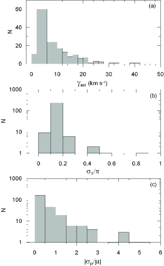
Fig. 1 : Distribution of $\gamma$ velocity errors (a), relative parallax errors (b) and relative proper motion errors (c) of the present CV sample.

2.2 Distances and proper motions

Although precise trigonometric parallaxes of some CVs were measured by many authors (Duerbeck, 1999; McArthur et al., 1999, 2001; Thorstensen, 2003; Beuermann et al., 2003, 2004; Harrison et al., 2004; Roelofs et al., 2007; Thorstensen et al., 2008, 2009), the measured number of parallaxes is only about 30. Therefore, parallaxes of CVs were collected in the following way as a general rule. Trigonometric parallaxes were taken as they are, where available. A new PLCs relation, which uses $J$, $K_{s}$ and $W$1 magnitudes in the Two Micron All Sky Survey (2MASS; Skrutskie et al., 2006) and Wide-field Infrared Survey Explorer ($WISE$; Wright et al., 2010) photometry and the orbital periods, was established by Özdönmez et al. (2015) in order to estimate the distances of 313 CVs. This new PLCs relation, which is valid in the ranges $1.37\leq P$(h) $\leq 12$, $0.13\leq(J-K_{s})_{0}\leq 1.01$, $-0.36\leq(K_{s}-W1)_{0}\leq 0.82$ and $2.9<M_{J}<10.4$ mag, was used to estimate the distances for CVs for which trigonometric parallaxes are not available. Here the subscript “0” denotes de-reddened colours. If a CV is out of the validity limits, then, the previous PLCs relation by Ak et al. (2007a), involving the 2MASS photometry, was used. For detailed descriptions of the methods see Ak et al. (2007a, 2008) and Özdönmez et al. (2015). Near and middle infrared magnitudes were taken from Cutri et al. (2003, 2012). Parallaxes of CVs were calculated using their distances with the well-known formula $\pi(mas)=1000/d($pc$)$. CVs with orbital periods ($P$) longer than 12 h were discarded since a CV with orbital period longer than this limit possibly contains a secondary star on its way to becoming a red giant (Hellier, 2001). Systems with $P<80$ min were not included in our preliminary sample, as well, because these systems must contain a degenerate secondary star.

The proper motions of the CVs in this study were taken from the UCAC4 Catalogue of Zacharias et al. (2013), the PPMXL Catalogue of Roeser et al. (2010), the Tycho-2 Catalogue of Høg et al. (2000), and from the re-reduced $Hipparcos$ catalogue of van Leeuwen (2007). Fig. 1b-c show the distribution of relative parallax errors and relative proper motion errors, respectively. The median value and standard deviation of relative parallax errors are 0.14 and $\pm$0.11, respectively. The median value and standard deviation of proper motion errors are 0.34 and $\pm$0.94 mas, respectively. Parallaxes and proper motion components are listed in Table 1 together with observational uncertainties. The columns of the table are organized as name, equatorial coordinates, type of the CV, orbital period, parallax, proper motion components, and $\gamma$ velocity. The types, equatorial coordinates and orbital periods of CVs in Table 1 were taken from Ritter & Kolb (2003, Edition 7.7).

2.3 Galactic space velocities

The algorithms and transformation matrices of Johnson & Soderblom (1987) were used to compute the space velocities with respect to the Sun. Equatorial coordinates ($\alpha$, $\delta$), proper motion components ($\mu_{\alpha}\cos\delta$, $\mu_{\delta}$), systemic velocity ($\gamma$) and the parallax ($\pi$) are the basic input data required. The form of this input data is adopted for the epoch of J2000 as described in the International Celestial Reference System (ICRS) of the $Hipparcos$ and the $Tycho$ Catalogues (ESA, 1997). The transformation matrices of Johnson & Soderblom (1987) use the notation of the right handed system. Therefore, the $U$, $V$ and $W$ are the components of a velocity vector of a star with respect to the Sun, where the $U$ is directed toward the Galactic Center ($l=0^{o},b=0^{o}$), the $V$ is in the direction of the Galactic rotation ($l=90^{o},b=0^{o}$), and the $W$ is towards the North Galactic Pole ($b=90^{o}$). Here, $l$ and $b$ are the Galactic longitude and latitude, respectively. Although CVs in the sample are relatively close objects, that is in the Solar neighbourhood, corrections for differential Galactic rotation were applied to the space velocities as described in Mihalas & Binney (1981). Galactic space velocity components were also corrected for the Local Standard of Rest (LSR) by adding the space velocity of the Sun to the space velocity components of CVs. The adopted space velocity of the Sun is $(U,V,W)_{\odot}=(8.50,13.38,6.49)$ km s^-1 (Coşkunoğlu et al., 2011).

The uncertainties of the space velocity components were computed by propagating the uncertainties of the input data with the algorithm given by Johnson & Soderblom (1987). The uncertainties of the total space velocities ($S_{err}=(U_{err}^{2}+V_{err}^{2}+W_{err}^{2})^{1/2}$) were also calculated. The histograms of the propagated uncertainties of total space velocities ($S_{err}$) and their components ($U_{err},V_{err},W_{err}$) are displayed in Fig. 2 with unshaded areas. The median and standard deviation of the total space velocity uncertainties in Fig. 2a are 15 and $\pm$15 km s^-1, respectively.

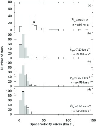
Fig. 2 : The histograms of the propagated uncertainties of total space velocities ($S_{err}$), and their components ($U_{err},V_{err},W_{err}$). Unshaded areas are for the preliminary sample, shaded areas for the refined sample.

As the space velocity dispersions and kinematical ages can be biased by the space velocities with very large uncertainties, we decided to remove all CVs with $S_{err}>30$ km s^-1, which corresponds to the median plus standard deviation of the space velocity uncertainties, in order to refine the CV sample in this study. This limit is indicated with an arrow in Fig. 2a. CVs with errors above this limit were discarded, thus 216 CVs were left in the refined sample. Shaded areas in Fig. 2b-d display the histograms of the uncertainties of the space velocity components ($U_{err},V_{err},W_{err}$) calculated for CVs in the refined sample. The mean values and dispersions of space velocity components calculated for the CV groups are given in Table 3. The median values of the errors for the refined sample are $\widetilde{U}_{err}=7.23$, $\widetilde{V}_{err}=7.39$ and $\widetilde{W}_{err}=6.86$ km s^-1 while error distributions have standard deviations $\pm 3.96$, $\pm 4.59$ and $\pm 4.29$ km s^-1, respectively for the $U$, $V$ and $W$ components of the space velocity.

2.4 Population analysis

In order to investigate kinematical and dynamical properties of CVs in the thin disc, thick disc and halo components of the Galaxy, a precise population analysis must be done. Here we adopt a pure dynamical approach to find population types of CVs in the refined sample. This approach is based on Galactic orbits of CVs. A similar method described in Ak et al. (2013) was used. Therefore, we first perform test-particle integration in a Milky Way potential which consists of a logarithmic halo of the form

$$\Phi_{\rm halo}(r)=v_{0}^{2}\ln\left(1+\frac{r^{2}}{d^{2}}\right).$$ (1)

Here, $v_{0}=186$ km s^-1 and $d=12$ kpc. A Miyamoto-Nagai potential represents the disc:

$$\Phi_{\rm disc}(R,z)=-\frac{GM_{\rm d}}{\sqrt{R^{2}+\left(a_{d}+\sqrt{z^{2}+b_{d}^{2}}\right)^{2}}},$$ (2)

with $M_{\rm d}=10^{11}~{}M_{\odot}$, $a_{d}=6.5$ kpc and $b_{d}=0.26$ kpc. Finally, the bulge is modelled as a Hernquist potential,

$$\Phi_{\rm bulge}(r)=-\frac{GM_{\rm b}}{r+c},$$ (3)

using $M_{\rm b}=3.4\times 10^{10}~{}M_{\odot}$ and $c=0.7$ kpc. A good representation of the Milky Way is obtained with the superposition of these components. The orbital period of the LSR is taken $P=2.18\times 10^{8}$ years while $V_{c}=222.5$ km s^-1 represents the circular rotational velocity at the Solar Galactocentric distance, $R_{0}=8$ kpc (Coşkunoğlu et al., 2012; Bilir et al., 2012).

The population types of CVs were determined according to the maximum vertical distances from the Galactic plane ($Z_{max}$) for their calculated orbits within the integration time of 3 Gyr, i.e. backwards in time. This integration time corresponds to 12-15 revolutions around the Galactic center so that the averaged orbital parameters can be determined reliably. Although the thick disc component of the Galaxy was discovered more than 30 years ago (Gilmore & Reid, 1983), there is still not a consensus for the numerical values of the parameters of this component. Especially, there is a degeneracy between the space density in the Solar Neighbourhood and the scale height of the thick disc component (Siegel et al., 2002; Karaali et al., 2004; Bilir et al., 2006, 2008). Thus, we have decided to find a value for $Z$ (distance from the Galactic plane), for which the space densities of thin and thick discs are almost equal, by performing Monte Carlo simulations with a wide range of parameters. For the Monte Carlo simulations in this study, wide ranges for the Solar space density and exponential scale height of the thick disc are adopted: 0% $\leq n_{TK}\leq$ 15% and 500 $\leq H_{TK}\leq$ 1500 pc, respectively. The adopted exponential scale height range for the thin disc is 200 $\leq H_{TN}\leq$ 350 pc. Here, the subscripts TK and TN refer to the thick disc and the thin-disc components of the Galaxy, respectively. These parameter ranges were taken from Ak et al. (2007b), who constructed a table of estimated parameters for the thin and thick discs from the literature. After 50000 trials for the Monte Carlo simulations, a histogram of the $Z$ values is obtained (Fig. 3). The mode value of 825 pc estimated from this histogram shows where the spatial densities of thin and thick discs are the most probably equal. This value is in agreement with those found in previous studies in which the deep sky surveys were used; cf. Ojha et al. (1999) (0.79 kpc), Siegel et al. (2002) (0.7-1 kpc), Karaali et al. (2004) (0.80-0.97 kpc), Bilir et al. (2006) (0.7-0.82 kpc).

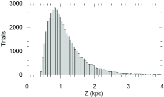
Fig. 3 : Distribution of the vertical distances from the Galactic plane ($Z$), where space densities of the thin and thick discs are almost equal, obtained from the Monte Carlo simulations with 50000 trials for a wide range of Galactic model parameters.

Thus, in this study the CVs with $Z_{max}\leq$ 825 pc are classified as thin-disc (TN) systems, while CVs with $Z_{max}>$ 825 pc are selected as thick disc or halo (TK-H) systems. Using this criterion, we have found that 17 of 216 CVs in the refined sample belong to the thick disc or halo population of the Galaxy. The rest of the sample is consisted of the thin-disc systems. The population types of the CVs in this study are indicated in Table 2. The columns of Table 2 are organized as name, Galactic coordinates ($l,b$), the corrected $U$, $V$ and $W$ components of the space velocity, maximum vertical distance to the Galactic plane ($Z_{max}$) and population type (TN or TK-H).

Table 2 : The Galactic coordinates ($l,b$), corrected space velocity components ($U,V,W$), total space velocities ($S$), maximum vertical distances from the Galactic plane of calculated orbits ($Z_{max}$) and population types (Pop) of CVs in the preliminary sample. In the “Pop” column, TN and TK-H refers to thin disc and thick disc-or-halo CVs. Full table can be obtained electronically.

ID	Name	$l$	$b$	$U$	$U_{err}$	$V$	$V_{err}$	$W$	$W_{err}$	$S$	$S_{err}$	$Z_{max}$	Pop
		(∘)	(∘)	(km s-1)	(km s-1)	(km s-1)	(km s-1)	(km s-1)	(km s-1)	(km s-1)	(km s-1)	(kpc)
1	WW Cet	90.007	-71.743	-15.69	6.97	23.55	4.17	-14.27	6.01	31.69	10.10	0.312	TN
2	V592 Cas	118.603	-6.910	9.14	8.52	41.25	12.55	0.81	6.03	42.26	16.32	0.048	TN
3	V709 Cas	120.042	-3.455	21.46	3.86	-21.83	3.32	6.20	2.93	31.23	5.87	0.077	TN
4	PX And	116.992	-36.335	37.23	14.28	-2.11	19.35	-9.69	17.73	38.53	29.88	0.539	TN
5	LTT 560	194.612	-88.105	19.94	2.69	-133.76	19.94	-29.18	0.73	138.35	20.13	0.395	TN
…	…	…	…	…	…	…	…	…	…	…	…	…	…
…	…	…	…	…	…	…	…	…	…	…	…	…	…
…	…	…	…	…	…	…	…	…	…	…	…	…	…

Representations of Galactic orbits, which are likely thick disc or halo CVs projected onto $X-Y$ and $X-Z$ planes, are shown in Fig. 4 and a list of these CVs are given in Table 4. $X$, $Y$ and $Z$ are heliocentric Galactic coordinates directed towards the Galactic Centre, Galactic rotation and the North Galactic Pole, respectively. The mean Galactocentric distances ($R_{m}$), and planar ($e_{p}$) and vertical ($e_{v}$) orbital eccentricities of Galactic orbits calculated for thick disc or halo CVs are also given in Table 4. $R_{m}$ is defined as the arithmetic mean of the final perigalactic ($R_{p}$) and apogalactic ($R_{a}$) distances of the Galactic orbit (Vidojevic & Ninkovic, 2009), and $Z_{max}$ and $Z_{min}$ are the maximum and minimum distances, respectively, to the Galactic plane. $e_{p}$ and $e_{v}$ are defined as $e_{p}=(R_{a}-R_{p})/(R_{a}+R_{p})$ and $e_{v}=(|Z_{max}|+|Z_{min}|)/R_{m}$, respectively. The computed space velocity components of the magnetic and non-magnetic CVs in the refined sample are compared in the velocity space in Fig. 5 according to the population types. As can be seen from Fig. 5, there is not a prominent difference between the velocity distributions of the magnetic and non-magnetic systems. In addition, thick-disc and halo CVs have higher $W$ velocities in the $V-W$ distribution (Fig. 5d) as compared to thin-disc stars.

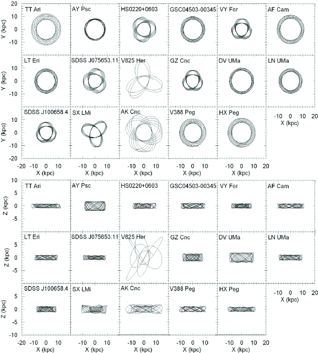
Fig. 4 : Representations of the Galactic orbits computed for the likely 17 thick disc or halo CVs projected onto $X-Y$ and $X-Z$ planes. Galactic orbits were calculated for an integration time of 3 Gyr.

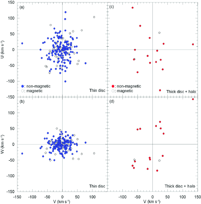
Fig. 5 : The computed space velocity components of the magnetic and non-magnetic CVs in the refined sample according to the population types.

2.5 Velocity dispersions and kinematical ages

Kinematical age of a group of stars can be calculated from the velocity dispersion of the systems using the formulae given by Wielen (1977). For CVs in this study, we have used the age-space velocity dispersion relation improved by Cox (2000):

$$\sigma_{\nu}^{3}(\tau)=\sigma_{\nu,\tau=0}^{3}+\frac{3}{2}\alpha_{V}\delta_{2}T_{\delta}\Biggl{[}\exp\Biggl{(}\frac{\tau}{T_{\delta}}\Biggl{)}-1\Biggr{]},$$ (4)

where $\sigma_{\nu,\tau=0}$ is the velocity dispersion at zero age, which is usually taken as 10 km s^-1 (Cox, 2000). $\alpha_{V}$ describes the rotation curve and it is taken approximately 2.95. $T_{\delta}$ is a time scale of $5\times 10^{9}$ yr and $\delta_{2}$ is a diffusion coefficient of $3.7\times 10^{-6}$ (km s${}^{-1})^{3}$ yr. $\sigma_{\nu}(\tau)$ and $\tau$ are the total velocity dispersion and the kinematical age of the CV group in question, respectively. The connection between the total dispersion of space velocity vectors ($\sigma_{\nu}$) and the dispersion of the velocity components is described as

$$\sigma_{\nu}^{2}=\sigma_{U}^{2}+\sigma_{V}^{2}+\sigma_{W}^{2}.$$ (5)

After computing $\sigma_{\nu}^{2}$ from the dispersions of velocity components, the kinematical age $\tau$ for a group of systems can be easily computed by replacing this total dispersion in Eq. (4). Assuming an isotropic distribution for the systems, the $\gamma$ velocity dispersion is defined $\sigma_{\gamma}^{2}=(1/3)\sigma_{\nu}^{2}$ (Wielen et al., 1992; van Paradijs et al., 1996). The $\gamma$ velocity dispersions of CV groups according to different orbital period regimes and population types are computed to compare with their theoretical predictions and listed in Table 3.

Table 3 : Mean space velocities, space velocity dispersions ($\sigma_{U}$, $\sigma_{V}$ and $\sigma_{W}$), total space velocity dispersions ($\sigma_{\nu}$), kinematical ages ($t$) and $\gamma$ velocity dispersions ($\sigma_{\gamma}$) of CV groups in the refined sample. “All sample” means all systems in the refined sample. M and nM denote magnetic (polars and intermediate polars) and non-magnetic systems, respectively. $N$ is the number of systems. TN represents thin-disc systems. The lower (2.15 h) and upper (3.18 h) borders for the period gap were adopted from Knigge (2006).

Parameter	$N$	$<U>$	$<V>$	$<W>$	$\sigma_{U}$	$\sigma_{V}$	$\sigma_{W}$	$\sigma_{\nu}$	$t$	$\sigma_{\gamma}$
		(km s-1)	(km s-1)	(km s-1)	(km s-1)	(km s-1)	(km s-1)	(km s-1)	(Gyr)	(km s-1)
All sample	216	-0.57$\pm$7.84	-3.60$\pm$8.49	-1.76$\pm$8.04	36.59$\pm$3.95	30.00$\pm$4.58	25.39$\pm$4.28	53.70$\pm$7.41	5.29$\pm$1.35	31.00$\pm$4.28
$Z_{max}\leq 825$ pc	199	0.02$\pm$7.50	-3.56$\pm$8.06	-1.23$\pm$7.62	33.91$\pm$3.85	27.61$\pm$4.41	18.15$\pm$4.04	47.35$\pm$7.11	4.13$\pm$1.27	27.34$\pm$4.10
$Z_{max}>825$ pc	17	-7.43$\pm$11.75	-4.13$\pm$13.48	-7.96$\pm$12.98	59.18$\pm$2.90	50.09$\pm$3.31	65.54$\pm$3.90	101.52$\pm$5.88	13.11$\pm$0.81	58.61$\pm$3.40
Magnetic (M,TN)	41	0.47$\pm$7.70	0.11$\pm$8.17	-1.24$\pm$8.18	38.53$\pm$4.52	33.10$\pm$4.48	22.60$\pm$4.21	55.60$\pm$7.63	5.64$\pm$1.39	32.10$\pm$4.41
Non-Magnetic (nM,TN)	158	-0.10$\pm$7.45	-4.51$\pm$8.04	-1.23$\pm$7.48	32.60$\pm$3.65	25.91$\pm$4.40	16.80$\pm$3.98	44.90$\pm$6.97	3.69$\pm$1.22	25.92$\pm$4.03
$P<2.15$ h (nM,TN)	46	-6.55$\pm$6.14	-6.11$\pm$6.86	0.74$\pm$5.97	30.65$\pm$3.21	23.93$\pm$3.92	18.85$\pm$3.21	43.21$\pm$6.00	3.40$\pm$1.03	24.95$\pm$3.46
$P>3.18$ h (nM,TN)	104	2.43$\pm$7.95	-3.85$\pm$8.51	-1.97$\pm$8.14	33.88$\pm$3.74	26.68$\pm$4.57	16.21$\pm$4.19	46.07$\pm$7.24	3.90$\pm$1.28	26.60$\pm$4.18
$P<2.15$ h (nM+M,TN)	56	-2.74$\pm$6.07	-3.03$\pm$6.84	-0.36$\pm$6.07	33.63$\pm$3.25	28.42$\pm$4.06	20.07$\pm$3.45	48.39$\pm$6.24	4.32$\pm$1.12	27.94$\pm$3.60
$P>3.18$ h (nM+M,TN)	128	1.64$\pm$8.13	-3.75$\pm$8.56	-2.44$\pm$8.37	34.62$\pm$4.03	27.03$\pm$4.58	17.00$\pm$4.23	47.10$\pm$7.42	4.09$\pm$1.32	27.19$\pm$4.29
$0.056<P(d)\leq 0.080$ (nM+M,TN)	48	-0.92$\pm$5.73	-3.47$\pm$6.55	-1.53$\pm$5.93	33.93$\pm$2.98	28.91$\pm$3.93	20.52$\pm$3.56	49.07$\pm$6.08	4.44$\pm$1.10	28.33$\pm$3.51
$0.080<P(d)\leq 0.150$ (nM+M,TN)	46	-3.51$\pm$8.40	-4.51$\pm$8.87	3.34$\pm$8.20	29.79$\pm$4.16	33.96$\pm$4.26	19.88$\pm$3.87	49.36$\pm$7.10	4.49$\pm$1.28	28.50$\pm$4.10
$0.150<P(d)\leq 0.210$ (nM+M,TN)	50	1.46$\pm$8.06	-5.50$\pm$8.12	-5.59$\pm$7.93	35.52$\pm$3.66	25.15$\pm$4.58	17.06$\pm$3.92	46.75$\pm$7.05	4.02$\pm$1.25	26.99$\pm$4.07
$0.210<P(d)\leq 0.350$ (nM+M,TN)	45	5.57$\pm$7.78	-5.02$\pm$8.79	-2.27$\pm$8.48	36.03$\pm$4.09	18.52$\pm$4.28	14.60$\pm$4.37	43.06$\pm$7.36	3.37$\pm$1.26	24.86$\pm$4.25
$0.350<P(d)\leq 0.500$ (nM+M,TN)	10	-11.46$\pm$7.89	16.65$\pm$8.10	5.71$\pm$7.68	27.97$\pm$3.05	26.59$\pm$5.19	7.55$\pm$3.57	39.32$\pm$6.98	2.74$\pm$1.13	22.70$\pm$4.03

3 Discussions

In order to investigate the kinematical properties of CVs, we have collected a sample of the systems with proper motions and systemic velocities. Unfortunately not many CVs have trigonometric parallaxes except only 30 close ones. After estimating the rest of the distances using improved PLCs relations by Özdönmez et al. (2015) and Ak et al. (2007a), their Galactic space velocity components were computed. A refined sample was constructed by eliminating CV’s with biggest errors $S_{err}>$ 30 km$s^{-1}$. In order to find out their Galactic population types, Galactic orbital parameters were computed. Additional sub-groups were formed in terms of their orbital periods.

Kinematical properties of all sample and sub-groups are summarized in Table 3. The dispersions of space velocity components obtained from the refined sample as a whole are $\sigma_{U}=36.59$ $\pm$ 3.95 km s^-1, $\sigma_{V}=30.00$ $\pm$ 4.58 km s^-1, $\sigma_{W}=25.39$ $\pm$ 4.28 km s^-1, indicating a mean kinematical age of 5.29 $\pm$ 1.35 Gyr. A systemic velocity ($\gamma$) dispersion of 31.00 $\pm$ 4.28 km s^-1 is obtained by evaluating the total space velocity dispersion ($\sigma_{\nu}=53.70$ $\pm$ 7.41 km s^-1) of the refined sample.

3.1 Groups according to population types

Galactic orbits of CVs in the refined sample shows that they are mostly located within the Galactic disc. Systems with vertical distances to the Galactic plane ($Z_{max}$) being larger than 825 pc are classified as the thick disc or halo CVs. We have found from the analysis of Galactic orbits that 199 of 216 CVs in the refined sample are members of the thin-disc component of the Galaxy. The rest are likely to be the thick disc or halo systems. It must be noted that our sample is consisted of the systems in the Solar Neighbourhood.

For further pinpointing the classification, we have calculated the planar ($e_{p}$) and vertical ($e_{v}$) orbital eccentricities of the Galactic orbits in addition to the maximum ($Z_{max}$) and minimum ($Z_{min}$) vertical distances to the Galactic plane (Table 4). Bilir et al. (2012) had found from the distribution of the vertical orbital eccentricity of red clump stars that the stars with $e_{v}\leq 0.12$ and $0.12<e_{v}\leq 0.25$ are the members of the thin and the thick disc populations of the Galaxy, respectively. Additionally, stars with $e_{v}>0.25$ are halo objects. $Z_{max}$ values of seven systems in Table 4 are larger than 825 pc, while their vertical orbital eccentricities are $e_{v}\leq$ 0.12. Thus, following the classification scheme of Bilir et al. (2012), we could conclude that these seven CVs can be in fact members of the old thin-disc population of the Galaxy. Nine of the 17 CVs in Table 4 are the thick-disc CVs. The total space velocity dispersion of the nine thick-disc CVs is found to be 93.87 $\pm$ 5.13 km s^-1, which corresponds to a kinematical age of 12.0 $\pm$ 0.8 Gyr consistent with the age of the thick-disc component of the Galaxy (Feltzing & Bensby, 2009). We have found one halo CV in our sample (V825 Her). The thick disc CVs in this study were not classified as the thick-disc members in Ak et al. (2013). Disagreement between this study and Ak et al. (2013) possibly results from the new $\gamma$ velocities, new distance estimation method and different approximation to classify the systems.

Table 4 : Names, types, orbital periods ($P$), perigalactic ($R_{p}$) and apogalactic ($R_{a}$) distances, the maximum ($Z_{max}$) and minimum ($Z_{min}$) vertical distances to the Galactic plane of calculated Galactic orbits for likely old thin disc, thick disc or halo stars in the refined sample. $e_{p}$ and $e_{v}$ denote planar and vertical orbital eccentricities of Galactic orbits for CVs. For the Type-1 and Type-2 columns, denotes are as described in Table 1. The most probable population types are indicated in the last column.

ID	Name	Type-1	Type-2	$P$	$R_{p}$	$R_{a}$	$Z_{max}$	$Z_{min}$	$e_{p}$	$e_{v}$	Pop. Type
				(h)	(kpc)	(kpc)	(kpc)	(kpc)
1	TT Tri	NL	nM	3.3513	7.750	12.226	0.834	-0.833	0.22	0.08	Old thin disc
2	AY Psc	DN	nM	5.2157	7.491	8.705	1.770	-1.769	0.07	0.22	Thick Disc
3	HS 0220+0603	NL	nM	3.5810	5.344	9.866	1.094	-1.090	0.30	0.14	Thick Disc
4	GSC 04503-00345	NL	nM	3.8758	7.773	9.979	1.043	-1.043	0.12	0.12	Old thin disc
5	VY For	NL	M	3.8064	4.823	8.403	0.923	-0.922	0.27	0.14	Thick Disc
6	AF Cam	DN	nM	7.7779	8.527	11.218	0.918	-0.919	0.14	0.09	Old thin disc
7	LT Eri	DN	nM	4.0841	7.325	9.549	1.014	-1.014	0.13	0.12	Old thin disc
8	SDSS J075653.11+085831.8	CV	nM	1.8960	5.224	9.774	0.871	-0.871	0.30	0.12	Old thin disc
9	AK Cnc	DN	nM	1.5624	6.612	15.251	1.850	-1.852	0.40	0.17	Thick Disc
10	GZ Cnc	DN	nM	2.1144	4.980	8.527	1.520	-1.519	0.26	0.23	Thick Disc
11	DV UMa	DN	nM	2.0605	8.359	10.136	1.892	-1.892	0.10	0.20	Thick Disc
12	LN UMa	NL	nM	3.4656	7.326	9.633	1.080	-1.079	0.14	0.13	Thick Disc
13	SDSS J100658.40+233724.4	DN	nM	4.4619	5.023	8.344	1.092	-1.087	0.25	0.16	Thick Disc
14	SX LMi	DN	nM	1.6128	3.845	11.247	1.604	-1.603	0.49	0.21	Thick Disc
15	V825 Her	NL	nM	4.9440	7.839	32.136	8.930	-8.901	0.61	0.45	Halo
16	V388 Peg	NL	M	3.3751	7.278	11.010	1.091	-1.090	0.20	0.12	Old thin disc
17	HX Peg	DN	nM	4.8192	8.012	11.378	0.925	-0.923	0.17	0.10	Old thin disc

If seven likely old thin-disc CVs was included in the thin-disc group, number of the thin-disc CVs increase to 206. So, the space density of the thin-disc CVs increases to 95$\%$. Such a result would be in agreement with Ak et al. (2013) who claim 94$\%$ of Solar Neighbourhood CVs are thin-disc stars. This result is also in agreement with Peters (2008) who concluded that the kinematics of these systems are indicative of a thin-disc Galactic population. The space density of the thick-disc CVs in our sample ($\sim$5%) shows that the refined CV sample in this study is complete for the Solar Neighbourhood, since space density of thick-disc CVs is in agreement with those derived for the field stars (Robin et al., 1996; Buser et al., 1999; Bilir et al., 2006). So, we conclude that statistical studies using the refined sample in our study give reliable results.

Kinematical properties of the thin disc ($Z_{max}\leq 825$ pc) and thick disc or halo ($Z_{max}>825$ pc) CVs are listed in Table 3. Kinematical properties of these groups are very different from each other, as expected. Kinematical ages of the thin disc and thick disc or halo stars are 4.13 $\pm$ 1.27 and 13.11 $\pm$ 0.81 Gyr, respectively. Although number of systems used in the estimation is small, kinematical ages of the CV groups from different Galactic population groups are consistent with the age of the Galactic components (Wyse, 2013).

3.2 Magnetic and non-magnetic systems

Kinematical ages of magnetic systems (polars and intermediate polars) could be different than non-magnetic systems, since the evolution of the magnetic systems could be different than the evolution of non-magnetic CVs (Wu & Wickramasinghe, 1993; Webbink & Wickramasinghe, 2002; Schwarz et al., 2007). Thus, we have estimated the kinematical properties of the magnetic and the non-magnetic systems separately. Before doing this estimation, we have removed the thick disc and the halo CVs from the refined sample as the results can be biased by kinematics of these populations.

Our results in Table 3 shows that non-magnetic thin-disc systems are younger than magnetic CVs: their kinematical ages are 3.69 $\pm$ 1.22 and 5.64 $\pm$ 1.39 Gyr, respectively. Our results are roughly in agreement with those of Peters (2008) who estimated mean kinematical ages of $\geq$4 and $\geq$5 Gyr for non-magnetic and magnetic systems, respectively. However, Ak et al. (2010) found an age of 7.68 $\pm$ 1.44 Gyr for magnetic systems since they did not remove thick disc and halo CVs from their sample which biased the age estimates.

3.3 Groups according to orbital periods

Table 3 shows that the kinematical ages of non-magnetic thin-disc CVs below ($P<2.15$ h) and above ($P>3.18$ h) the orbital period gap, which are 3.40 $\pm$ 1.03 and 3.90 $\pm$ 1.28 Gyr, respectively. When we consider magnetic and non-magnetic thin-disc systems together, their ages are estimated as 4.32 $\pm$ 1.12 and 4.09 $\pm$ 1.32 Gyr for the systems below and above the gap, respectively.

Standard evolution theory predicts that the CVs above the period gap must be younger than the systems below the gap. If this is true, the kinematical properties of the non-magnetic thin-disc CVs must obey this rule in the absence of the bias from the thick disc or the halo systems. However, our results are not in agreement with this prediction. It is clear from Table 3 that there is not a considerable age difference between the thin-disc non-magnetic systems below and above the orbital period gap. Even if we include magnetic systems in the age calculation, which are considerably older than non-magnetic CVs, kinematical ages for the systems below and above the gap remain almost equal. These results are in agreement with Ak et al. (2010) and van Paradijs et al. (1996).

It is predicted from the age structure of a Galactic CV population obtained by applying standard formation and evolution models (Kolb & Stehle, 1996) that CVs above the orbital period gap must have an average age of 1 Gyr, while the mean age of systems below the gap should be 3-4 Gyr (see also Ritter & Burkert, 1986). This age difference is mainly due to the time spent evolving from the post-CE phase into the contact phase (Kolb, 2001). Although the age 3.40 Gyr derived for the systems below the gap is in agreement with the theoretical prediction, we can not find a 2-3 Gyr age difference for the systems above and below the gap.

In order to investigate the age differences between the various period regimes, we have divided the refined sample into smaller subsamples according to almost the same number of CVs at different period ranges. The total space velocity dispersions and corresponding kinematical ages for CVs in these period ranges are summarized in Table 3. $U-V$ diagrams for the systems in these period ranges are shown in Fig. 6. Unlike the age-period relation presented in Ak et al. (2010), Table 3 shows that the kinematical ages decrease towards longer orbital periods, as expected from the standard evolution theory, with a decreasing rate of $dP/dt=-1.62(\pm 0.15)\times 10^{-5}$ sec yr^-1. It seems that the systems near the upper border of the gap affect the mean age estimate of systems above the gap and increase the mean value, when all systems above the gap are taken into account as a CV group. Thus, we can conclude that the space velocity dispersion, and so the age, decreases as the orbital period increases.

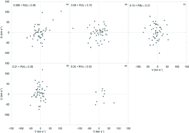
Fig. 6 : $U-V$ diagrams of CVs in the refined sample for different orbital period ranges.

3.4 The $\gamma$ velocity dispersion of CVs

The $\gamma$ velocity dispersions of CV sub-groups are useful tools to test predictions of the standard formation and evolution theory. The $\gamma$ velocity dispersion of all systems in the refined sample is estimated as $\sigma_{\gamma}=31.00\pm 4.28$ km s^-1. This value is not significantly different than $\sigma_{\gamma}=30\pm 4$ km s^-1 found by Ak et al. (2010). Kolb & Stehle (1996) predicted that the $\gamma$ velocity dispersions for the systems above and below the orbital period gap are $\sigma_{\gamma}\simeq 15$ and $\sigma_{\gamma}\simeq 30$ km s^-1, respectively. Prediction of Kolb (2001) states that the $\gamma$ velocity dispersions of CVs should be $\sigma_{\gamma}\simeq 27$ and $\sigma_{\gamma}\simeq 32$ km s^-1 for the systems above and below the gap, respectively, if magnetic braking does not operate in the detached phase. These theoretical predictions suggest that there must be considerable difference for the $\gamma$ velocity dispersions of CVs below and above the orbital period gap. In order to compare with these theoretical predictions, we have calculated the $\gamma$ velocity dispersions for all thin-disc systems below and above the period gap, and found $\sigma_{\gamma}=27.94\pm 3.60$ km s^-1 and $\sigma_{\gamma}=27.19\pm 4.29$ km s^-1, respectively. Although the theoretically predicted dispersion for CVs below the gap is roughly in agreement with observations, it is clear that CVs below and above the gap have $\gamma$ velocity dispersions that are the same, within the errors. A substantial amount of difference between the $\gamma$ velocity dispersions of the systems below and above the gap can not be obtained, as well, even if we use only non-magnetic thin-disc CVs (Table 3): $\sigma_{\gamma}=24.95\pm 3.46$ and $\sigma_{\gamma}=26.60\pm 4.18$ km s^-1 for below and above the gap, respectively. Note that using only $\sigma_{U}$ and $\sigma_{V}$ for the calculation of total dispersion does not change this similarity between the $\gamma$ velocity dispersions.

4 Conclusions

By analysing available kinematical data of CVs, we have concluded that there is not considerable kinematical difference between the systems below and above the orbital period gap. This result is not in agreement with the standard theory of the CV evolution and results of Ak et al. (2010). Thus, we can not confirm the prediction of Kolb & Stehle (1996) who predicted 2-3 Gyr mean age difference between the CVs below and above the period gap. Smaller age difference implies similar angular momentum loss time scales for systems with low-mass and high-mass secondaries (Kolb, 2001). However, it must be noted that kinematical age of CV groups slightly increases with decreasing orbital period, a result in agreement with the standard theory of the CV evolution.

Observational $\gamma$ velocity dispersion of CVs below the period gap is roughly in agreement with the predictions of the standard theory CV evolution (Kolb & Stehle, 1996; Kolb, 2001). However, a substantial amount of difference for $\gamma$ velocity dispersions of the systems below and above the period gap could not be obtained from the observations.

By calculating Galactic orbital parameters of CVs in the sample, we found that 17 of them are likely members of old thin disc, thick disc or halo components of the Galaxy. Orbital eccentricities and maximum vertical distances to the Galactic plane show that only one of them is a halo CV (V825 Her). From the population analysis based on a pure dynamical approximation, we have concluded that CVs are very consistent with the thin-disc population of the Galaxy.

5 Acknowledgments

Part of this work was supported by the Research Fund of the University of Istanbul, Project Numbers: 27839, 39170 and 39742. This work has been supported in part by the Scientific and Technological Research Council (TÜBİTAK) grand numbers: 111T224 and 212T091. This research has made use of the SIMBAD database, operated at CDS, Strasbourg, France. This research has made use of NASA’s Astrophysics Data System.

References

- Ak et al. (2007a) Ak, T., Bilir, S., Ak, S., Retter, A., 2007a. NewA 12, 446.
- Ak et al. (2007b) Ak, S., Bilir, S., Karaali, S., Buser, R., 2007b. Astron. Nachr. 328, 169.
- Ak et al. (2008) Ak, T., Bilir, S., Ak, S., Eker, Z., 2008. NewA 13, 133.
- Ak et al. (2010) Ak, T., Bilir, S., Ak, S., Coşkunoğlu, K.B., Eker, Z., 2010. NewA 15, 491.
- Ak et al. (2013) Ak, T., Bilir, S., Güver, T., Çakmak, H., 2013. NewA 22, 7.
- Bensby et al. (2003) Bensby, T., Feltzing, S., Lundström, I., 2003. A&A 410, 527.
- Bensby et al. (2005) Bensby, T., Feltzing, S., Lundström, I., Ilyin, I., 2005. A&A 433, 185.
- Beuermann et al. (2003) Beuermann, K., Harrison, T.E., McArthur, B.E., Benedict, G.F., Gänsicke, B.T., 2003. A&A 412, 821.
- Beuermann et al. (2004) Beuermann, K., Harrison, T.E., McArthur, B.E., Benedict, G.F., Gänsicke, B.T., 2004. A&A 419, 291.
- Bilir et al. (2006) Bilir, S., Karaali, S., Gilmore, G., 2006. MNRAS 366, 1295.
- Bilir et al. (2008) Bilir, S., Cabrera-Lavers, A., Karaali, S., Ak, S., Yaz, E., López-Corredoira, M., 2008. PASA 25, 69.
- Bilir et al. (2012) Bilir, S., Karaali, S., Ak, S., Önal, Ö., Dağtekin, N.D., Yontan, T., Gilmore, G., Seabroke, G.M., 2012. MNRAS 421, 3362.
- Buser et al. (1999) Buser, R., Rong, J., Karaali, S., 1999. A&A 348, 98.
- Coşkunoğlu et al. (2011) Coşkunoğlu, B., et al., 2011. MNRAS 412, 1237
- Coşkunoğlu et al. (2012) Coşkunoğlu, B., Ak, S., Bilir, S., Karaali, S., Önal, Ö., Yaz, E., Gilmore, G., Seabroke, G.M., 2012. MNRAS 419, 2844
- Cox (2000) Cox, A.N., 2000. Allen’s astrophysical quantities, New York: AIP Press; Springer, Edited by Arthur N. Cox. ISBN: 0387987460.
- Cutri et al. (2003) Cutri, R.M., et al., 2003. VizieR On-line Data Catalog: II/246. Originally published. In: University of Massachusetts and Infrared Processing and Analysis Center, (IPAC/ California Institute of Technology).
- Cutri et al. (2012) Cutri, R.M., et al., 2012. WISE All-Sky Data Release, VizieR Online Data Catalog, 2311.
- Duerbeck (1999) Duerbeck, H.W., 1999. IBVS No.4731.
- ESA (1997) ESA, 1997. ESA SP-1200, The Hipparcos and Tycho Catalogues. ESA, Noordwijk
- Feltzing & Bensby (2009) Feltzing, S., Bensby, T., 2009. The Ages of Stars, Proceedings of the International Astronomical Union, IAU Symposium, Vol. 258, p.23-30.
- Gänsicke et al. (2009) Gänsicke, B.T., et al., 2009. MNRAS 397, 2170.
- Gilmore & Reid (1983) Gilmore, G., Reid N., 1983. MNRAS 202, 1025.
- Hameury et al. (1988) Hameury, J.M., King, A.R., Lasota, J.P., Ritter, H., 1988. ApJ 327, 77.
- Harrison et al. (2004) Harrison, T.E., Johnson, J.J., McArthur, B.E., Benedict, G.F., Szkody, P., Howell, S.B., Gelino, D.M., 2004. AJ 127, 460.
- Hellier (2001) Hellier, C., 2001. Cataclysmic Variable Stars, How and why they vary, Springer-Praxis Books in astronomy and space sciences, Cornwall,UK.
- Høg et al. (2000) Høg, E., Fabricius, C., Makarov, V.V., Urban, S., Corbin, T., Wycoff, G., Bastian, U., Schwekendiek, P., Wicenec, A., 2000. A&A 355, 27.
- Johnson & Soderblom (1987) Johnson, D.R.H., Soderblom, D.R., 1987. AJ 93, 864.
- Karaali et al. (2004) Karaali, S., Bilir, S., Hamzaoğlu, E., 2004. MNRAS 355, 307.
- Kolb (2001) Kolb, U., 2001. in The influence of binaries on stellar population studies, Astrophysics and Space Science Library (ASSL), Vol. 264, 321.
- Kolb & Stehle (1996) Kolb, U., Stehle, R., 1996. MNRAS 282, 1454.
- King (1988) King, A.R., 1988. QJRAS 29, 1.
- Knigge (2006) Knigge, C., 2006. MNRAS 373, 484.
- Knigge (2011) Knigge, C., 2011. Evolution of compact binaries. ASP Conference Proceedings, Vol. 447, Linda Schmidtobreick, Matthias R. Schreiber, and Claus Tappert (eds.), 3.
- McArthur et al. (1999) McArthur, B.E., et al., 1999. ApJ 520, L59.
- McArthur et al. (2001) McArthur, B.E., et al., 2001. ApJ 560, 907.
- Mihalas & Binney (1981) Mihalas, D., Binney, J., 1981. in Galactic Astronomy, 2nd edition, Freeman, San Fransisco.
- North et al. (2002) North, R.C., Marsh, T.R., Kolb, U., Dhillon, V.S., Moran, C.K.J., 2002. MNRAS 337, 1215.
- Ojha et al. (1999) Ojha, D.K., Bienaymé, O., Mohan V., Robin A.C., 1999. A&A 351, 945.
- Özdönmez et al. (2015) Özdönmez, A., Ak, T., Bilir, S., 2015. NewA 34, 234.
- Paczynski (1967) Paczynski, B., 1967. Acta Astron. 17, 287.
- Paczynski & Sienkiewicz (1983) Paczynski, B., Sienkiewicz, R., 1983. ApJ 268, 825.
- Peters (2007) Peters, C.S., 2007. Bulletin of the American Astronomical Society, 39, 817.
- Peters (2008) Peters, C.S., 2008. Kinematics and Space Densities for the Local Cataclysmic Variable Population, PhD Thesis, United States – New Hampshire: Dartmouth College; 2008. Publication Number: AAT 3330605. Source: DAI-B 69/10.
- Pretorius et al. (2007) Pretorius, M.L., Knigge, C., Kolb, U., 2007. MNRAS 374, 1495.
- Rappaport et al. (1982) Rappaport, S., Joss, P.C., Webbink, R.F., 1982. ApJ 254, 616.
- Rappaport et al. (1983) Rappaport, S., Verbunt, F., Joss, P.C., 1983. ApJ 275, 713.
- Ritter & Burkert (1986) Ritter, H., Burkert, A., 1986. A&A 158, 161.
- Ritter & Kolb (2003) Ritter, H., Kolb, U., 2003. A&A 404, 301.
- Robin et al. (1996) Robin, A.C., Haywood, M., Créze, M., Ojha, D.K., Bienaymé, O., 1996. A&A 305, 125.
- Roelofs et al. (2007) Roelofs, G.H.A., Groot, P.J., Benedict, G.F., McArthur, B.E., Steeghs, D., Morales-Rueda, L., Marsh, T.R., Nelemans, G., 2007. ApJ 666, 1174.
- Roeser et al. (2010) Roeser, S., Demleitner, M., Schilbach, E., 2010. AJ 139, 2440.
- Schwarz et al. (2007) Schwarz, R., Schwope, A.D., Staude, A., Rau, A., Hasinger, G., Urrutia, T., Motch, C., 2007. A&A 473, 511.
- Siegel et al. (2002) Siegel, M.H., Majewski, S.R., Reid, I.N., Thompson, I.B., 2002. ApJ 578, 151.
- Skrutskie et al. (2006) Skrutskie, M.F., et al., 2006. AJ 131, 1163.
- Spruit & Ritter (1983) Spruit, H.C., Ritter, H., 1983. A&A 124, 267.
- Thorstensen (2003) Thorstensen, J.R., 2003. AJ 126, 3017.
- Thorstensen et al. (2008) Thorstensen, J.R., Lépine, S., Shara, M., 2008. AJ 136, 2107.
- Thorstensen et al. (2009) Thorstensen, J.R., Schwarz, R., Schwope, A.D., Staude, A., Vogel, J., Krumpe, M., Kohnert, J., Nebot Goḿez-Morań, A., 2009. PASP 121, 465.
- van Leeuwen (2007) van Leeuwen, F., 2007. A&A 474, 653.
- van Paradijs et al. (1996) van Paradijs, J., Augusteijn, T., Stehle, R., 1996. A&A 312, 93.
- Verbunt & Zwaan (1981) Verbunt, F., Zwaan, C., 1981. A&A 100, L7.
- Vidojevic & Ninkovic (2009) Vidojevic, S., Ninkovic, S., 2009. AN 330, 46.
- Webbink & Wickramasinghe (2002) Webbink, R.F., Wickramasinghe, D.T., 2002. MNRAS 335, 1.
- Wielen (1977) Wielen, R., 1977. A&A 60, 263.
- Wielen et al. (1992) Wielen, R., Dettbarn, C., Fuchs, B., Jahreiss, H., Radons, G., 1992. in The Stellar Populations of Galaxies, IAU Symp. 149, B. Barbuy, A. Renzini (eds.), 81.
- Willems et al. (2005) Willems, B., Kolb, U., Sandquist, E.L., Taam, R.E., Dubus, G., 2005. ApJ 635, 1263.
- Wright et al. (2010) Wright, E.L., et al., 2010. AJ 140, 1868.
- Wu & Wickramasinghe (1993) Wu, K., Wickramasinghe, D.T., 1993. MNRAS 265, 115.
- Wyse (2013) Wyse, R.F.G., 2013. Planets, Stars and Stellar Systems Vol. 5, by Oswalt, T.D. and Gilmore, G., ISBN 978-94-007-5611-3. Springer Science+Business Media Dordrecht, p.1.
- Zacharias et al. (2013) Zacharias, N., Finch, C.T., Girard, T.M., Henden, A., Bartlett, J.L., Monet, D.G., Zacharias, M.I., 2013. AJ 145, 44.