Application of axiomatic formal theory to the Abraham–Minkowski controversy

Abstract

A transparent linear dielectric in free space that is illuminated by a finite quasimonochromatic field is a thermodynamically closed system. The energy–momentum tensor that is derived from Maxwellian continuum electrodynamics for this closed system is inconsistent with conservation of momentum; that is the foundational issue of the century-old Abraham–Minkowski controversy. The long-standing resolution of the Abraham–Minkowski controversy is to view continuum electrodynamics as a subsystem and write the total energy–momentum tensor as the sum of an electromagnetic energy–momentum tensor and a phenomenological material energy–momentum tensor. We prove that if we add a material energy–momentum tensor to the electromagnetic energy–momentum tensor, in the prescribed manner, then the total energy, the total linear momentum, and the total angular momentum are constant in time, but other aspects of the conservation laws are violated. Specifically, the four-divergence of the total (electromagnetic plus material) energy–momentum tensor is self-inconsistent and violates Poynting’s theorem. Then, the widely accepted resolution of the Abraham–Minkowski dilemma is proven to be manifestly false. The fundamental physical principles of electrodynamics, conservation laws, and special relativity are intrinsic to the vacuum; the extant dielectric versions of physical principles are non-fundamental extrapolations from the vacuum theory. Because the resolution of the Abraham–Minkowski momentum controversy is proven false, the extant theoretical treatments of macroscopic continuum electrodynamics, dielectric special relativity, and energy–momentum conservation in a simple linear dielectric are mutually inconsistent for macroscopic fields in matter. We derive mutually consistent theoretical treatments of physical processes in an isotropic, homogeneous, linear dielectric-filled, flat, non-Minkowski, continuous material spacetime. The Abraham–Minkowski momentum controversy has a robust resolution in the new Lagrangian field theory of continuum electrodynamics.

I Introduction

I.1 Physical Setting

The foundations of the energy–momentum tensor and the associated tensor-based spacetime conservation theory come to electrodynamics from classical continuum dynamics where the divergence theorem is applied to a Taylor series expansion of the density field of an intrinsic property (e.g., mass, particle number) of an unimpeded, inviscid, incoherent flow of non-interacting particles (molecules, dust, etc.) in the continuum limit (fluid or particle number field, for example) in an otherwise empty volume BIFox . Although the continuous formulation of conservation principles was originally the provenance of fluid mechanics (continuum dynamics), the energy and momentum conservation properties of light propagating in the vacuum were long-ago cast in the energy–momentum tensor formalism in which the light field (flow of non-interacting photons in the continuum limit) plays the role of the continuous fluid BILL . However, extending the tensor-based theory of energy–momentum conservation of the continuous light field in the vacuum to propagation of the light field in a linear dielectric medium, also in the continuum limit, has proven to be persistently problematic, as exemplified by the more-than-century-old Abraham–Minkowski momentum controversy BIMin ; BIAbr ; BIRL ; BIBrev ; BIAMC3 ; BIKemplatest ; BIPfei ; BIAMC2 ; BIAMC4 ; BIAMC5 ; BIObuk ; BIObuk2 ; BIMuka ; BIMuka2 ; BIBarn ; BIPeierls ; BIBalazs ; BIGord ; BIMol ; BIBahder ; BIJMP ; BISPIE ; BIBrev2 ; BINewExp1 ; BINewExp2 ; BISheMan ; BISheBrev ; BIBethune ; BIBrevnew ; BIBrevnew2 .

The origin story of the Abraham-Minkowski controversy is that the Minkowski energy–momentum tensor is not diagonally symmetric. Motivated by the need to preserve the principle of conservation of angular momentum, Abraham symmetrized the energy–momentum tensor by an ad hoc redefinition of the linear momentum density to be the Poynting energy flux vector divided by $c^{2}$. The issue of the lack of symmetry in the Minkowski energy–momentum tensor has since been overtaken by substantive problems with conservation of linear momentum for both the Minkowski and Abraham energy–momentum tensors. The modern resolution of the Abraham–Minkowski momentum controversy is to decide that the electromagnetic energy, the electromagnetic angular momentum, and the electromagnetic linear momentum are features of an electromagnetic subsystem. The addition of a phenomenological material subsystem completes the total system. Although the “modern” resolution BIGord ; BIPenHaus has been around for 50 years, or so, it still isn’t working out quite right.

A gradient-index antireflection-coated right rectangular block of a simple (absorption-negligible, isotropic, homogeneous, lowest-order dispersive) linear dielectric material, with refractive index $n$, situated in free-space that is illuminated at normal incidence by a finite quasimonochromatic field with center frequency $\omega_{p}$ is a thermodynamically closed system that consists of the field, the dielectric material, and any other pertinent subsystems. Integrating over all-space $\Sigma$, the Abraham (linear) momentum

$${\bf G}_{A}=\int_{\Sigma}\frac{{\bf E}\times{\bf B}}{c}dv$$ (1)

and the Minkowski (linear) momentum

$${\bf G}_{M}=\int_{\Sigma}\frac{n^{2}{\bf E}\times{\bf B}}{c}dv$$ (2)

are not constant in time as a finite electromagnetic pulse enters the dielectric from the vacuum BIBrev ; BIAMC3 ; BIKemplatest ; BIPfei ; BIAMC2 . The fact that the electromagnetic momentum is not conserved means that a portion of the incident electromagnetic momentum is being transferred to some other subsystem and the dielectric material is the only other identifiable component of the system.

When the field is entirely within an antireflection-coated block of a homogeneous simple linear medium, the Abraham momentum is less than the incident (from vacuum) momentum by a nominal factor of $n$. The Minkowski momentum is greater than the Abraham momentum by a factor of $n^{2}$ and it is therefore greater than the (vacuum) incident momentum by a factor of $n$. The fact that neither the Abraham momentum nor the Minkowski momentum is globally conserved is well-known in the scientific literature BIBrev . Nevertheless, many researchers BIPfei ; BIObuk justifiably claim that the Minkowski (linear) momentum is conserved or “almost” conserved based on the four-divergence of the Minkowski energy–momentum tensor being negligible, which corresponds to a local conservation law BIGiu , $\partial_{\beta}{\sf T}^{i\beta}=0$, see Eq. (47). But, a factor of $n$ is not a perturbation and any claim BIPfei ; BIObuk that the Minkowski momentum (or the Minkowski tensor) is conserved or “almost” conserved is manifestly false based on the global conservation condition BIGiu ; BILL , $P^{i}(t)=P^{i}(t_{0})$, see Eq. (48). Pfeifer, Nieminen, Heckenberg, and Rubinsztein-Dunlop BIPfei present both facts from the extant literature in their comprehensive review article showing that the Minkowski momentum is greater than the incident momentum by a factor of $n$ in their Sec. 9A and noting that the Minkowski momentum is almost conserved in their Sec. 8C. This unremarked contradiction between local and global conservation laws BIGiu , appears to be one of many factors that contribute to the extraordinary longevity of the Abraham–Minkowski controversy.

In time gone by, the necessity for a medium in which light waves propagate proved the existence of the ether. The properties of the ether, including ether drag and partial ether drag, were determined from the observed characteristics of light propagation in the vacuum. Likewise, the necessity for global conservation of linear momentum in a thermodynamically closed field-plus-matter system proves the existence of a material momentum that is associated with the movement of matter in a microscopic picture of a dielectric substructure BIAMC3 ; BIKemplatest ; BIPfei ; BIAMC2 . We note that such a microscopic subsystem is adverse to the continuum limit that is a foundational concept of continuum electrodynamics. Nevertheless, the assumption of identifiable electromagnetic and material component subsystem momentums is commonly made and assumed to be settled physics in the scientific literature BIAMC3 ; BIKemplatest ; BIPfei ; BIAMC2 . However, the nature of the material subsystem is elusive and controversial.

While the physical origin and characteristics of the phenomenological material momentum have been debated for many decades, experimental demonstrations of a material momentum have been variously inconsistent, contradictory, and refuted BIBrev ; BIBrev2 ; BINewExp1 ; BINewExp2 ; BISheMan ; BISheBrev ; BIBethune . Likewise, theoretical treatments of the Abraham–Minkowski controversy BIAMC3 ; BIKemplatest ; BIPfei ; BIAMC2 ; BIAMC4 ; BIAMC5 ; BIObuk ; BIObuk2 ; BIMuka ; BIMuka2 ; BIBarn ; BIPeierls ; BIBalazs ; BIGord ; BIMol ; BIBahder ; BIJMP ; BISPIE have not provided a consistent physical solution. In 2007, Pfeifer, Nieminen, Heckenberg, and Rubinsztein-Dunlop BIPfei reviewed the state of the field and concluded that the issue had been settled for some time: “When the appropriate accompanying energy–momentum tensor for the material medium is also considered, experimental predictions of the various proposed tensors will always be the same, and the preferred form is therefore effectively a matter of personal choice.” Three years later, Barnett BIBarn offered a more restrictive resolution of the Abraham–Minkowski debate by contending that the total momentum ${\bf G}_{total}$ for the medium and the field is composed of either the Minkowski canonical momentum ${\bf G}_{M}$ or the Abraham kinetic momentum ${\bf G}_{A}$ supplemented by the appropriate canonical material momentum ${\bf G}_{can}$ or kinetic material momentum ${\bf G}_{kin}$. Although the Barnett BIBarn and Pfeifer, Nieminen, Henckenberg, and Rubinsztein-Dunlop BIPfei theories are based on fundamental principles, Barnett’s restriction to two simultaneous physically motivated electromagnetic momentums is contradicted by the mathematical tautology that underlies the analysis of Pfeifer, et al., and vice-versa.

In order to present a concrete example for discussion, we use the common Barnett BIBarn model for the field and matter components of the total energy–momentum tensor. The material momentums are constructed such that the total (electromagnetic plus material) linear momentum BIAMC2 ; BIBarn

$${\bf G}_{total}={\bf G}_{incident}={\bf G}_{em}+{\bf G}_{material}$$ (3a)

$${\bf G}_{total}={\bf G}_{A}+{\bf G}_{kin}={\bf G}_{M}+{\bf G}_{can}$$ (3b)

of a finite pulse of the continuous light field in a continuous simple linear dielectric material with no other consequential subsystems is constant in time as required by global conservation BIPfei ; BIFox ; BILL ; BIGiu for a continuous fluid. Clearly, ${\bf G}_{kin}=(1-1/n){\bf G}_{incident}$ and ${\bf G}_{can}=(1-n){\bf G}_{incident}$ when the electromagnetic pulse is fully within an antireflection-coated, isotropic, homogeneous, transparent linear dielectric medium. The material energy is constructed such that the total (electromagnetic plus material) energy is equal to the incident energy BIPfei

$$U_{total}=U_{incident}=U_{em}+U_{material}$$ (4a)

$$U_{total}=U_{A}+U_{kin}=U_{M}+U_{can}$$ (4b)

and is constant in time as the light pulse propagates from the vacuum into the antireflection-coated material. The total energy–momentum tensor is the sum of the Abraham energy–momentum tensor and a kinetic material energy–momentum tensor. In addition, the total energy–momentum tensor is the sum of the Minkowski energy–momentum tensor and a canonical material energy–momentum tensor. That is BIPfei ,

$${\sf T}_{total}^{\alpha\beta}={\sf T}_{incident}^{\alpha\beta}={\sf T}_{em}^{\alpha\beta}+{\sf T}_{material}^{\alpha\beta}$$ (5a)

$${\sf T}_{total}^{\alpha\beta}={\sf T}_{A}^{\alpha\beta}+{\sf T}_{kin}^{\alpha\beta}={\sf T}_{M}^{\alpha\beta}+{\sf T}_{can}^{\alpha\beta}\,.$$ (5b)

Obviously, Brevik’s BIBrevnew admonitions against the application of conservation laws to subsystems do not apply to conservation of the total energy, the total linear momentum, the total angular momentum, or the total energy–momentum tensor of the complete and closed field-plus-matter system that is considered here and in Refs. BISPIE ; BIBahder ; BIJMP .

According to the Scientific Method, a scientific hypothesis must result in a unique testable prediction of physical quantities. There are many examples in the experimental record in which the interpretation of momentum experiments is unrestricted with experiments that prove the Minkowski electromagnetic momentum later being shown to prove the Abraham electromagnetic momentum and vice versa BIBrev . Likewise, experiments that disprove the Minkowski momentum are later re-analyzed to confirm the Minkowski momentum and similarly for the Abraham momentum BIBrev . The non-uniqueness of the electromagnetic momentum and the non-uniqueness of the material momentum for light in a dielectric are contrary to Popper’s criterion of falsifiability and constitute a violation of the Scientific Method.

The prior work appears to present a very complex situation because some experiments support the Abraham definition of momentum and other experiments support the Minkowski momentum formula. This might suggest that the Scientific Method needs to be malleable in order to accommodate the experimentally proven non-unique incommensurate momentums. However, appeal to complexity is a fallacious application of the Scientific Method. The problem is that electromagnetic momentum is not measured directly. Instead the force due to optical pressure on a mirror inserted in a fluid dielectric is measured and related to the change in electromagnetic momentum BIBrev ; BIPfei ; BIExp . Using the Abraham, Minkowski, or other momentum formula to relate the measured quantity (force) to the momentum creates a circular, self-proving theory, see Sec. 7.

We are accustomed to having well-designed experiments either prove or disprove scientific hypotheses. However, experiments cannot, in either principle or practice, provide a definitive resolution of the Abraham–Minkowski controversy BIBrevnew because the Scientific Method has been abrogated by the subsystem separation. In order to be theoretically definitive, the present work is based almost entirely on the unique, unseparated, globally conserved total (field plus matter plus other) momentum or the corresponding total momentum density of a thermodynamically closed system with appropriate system boundaries.

In a thermodynamically closed system, the total momentum, like the total energy, is a known quantity that is uniquely determined from the initial conditions by being constant in time. Then the total energy density and the total linear momentum density components of the total energy–momentum tensor are uniquely decided by time independence of the spatially integrated total energy and total momentum densities (global conservation law) BISPIE ; BIBahder ; BIJMP . The construction of the unique total (electromagnetic plus material plus other) energy–momentum tensor BISPIE ; BIBahder ; BIJMP from these total energy density and total momentum density components gets us congruent with the Scientific Method and definitively resolves the Abraham–Minkowski controversy. That is the generally accepted resolution of the Abraham–Minkowski controversy. Except that there are problems here, too. Applying the four-divergence operator to the unique total energy–momentum tensor, one obtains spacetime conservation laws in the form of continuity equations for the total energy and the total linear momentum BIPfei ; BISPIE ; BIBahder ; BIJMP . It is easily argued, on physical grounds, that the conservation law for the total energy that is obtained by applying the four-divergence operator to the total energy–momentum tensor cannot be incommensurate with the Poynting theorem that is systematically derived from the Maxwell–Minkowski field equations for a simple linear dielectric. It is also easily proven mathematically that i) the energy conservation law, derived from the four-divergence of the total energy–momentum tensor, is self-inconsistent because its two non-zero terms depend on different powers of the refractive index and ii) the conservation law for the total energy that is derived from the four-divergence of the total energy–momentum tensor is undeniably incommensurate with the Poynting theorem BIJMP . The contradiction of sound physical arguments by mathematical reality seems to also contribute to the longevity of the dispute.

In summary, we have “fixed” the Abraham–Minkowski momentum conservation problem in the prescribed manner BIPfei ; BIBarn only to have contradictions appear in a different form elsewhere. The current author BISPIE ; BIBahder ; BIJMP made the ansatz of a Ravndal BIFinn refractive index-dependent material four-divergence operator and demonstrated consistency between the field equations and total energy–momentum conservation laws, at the cost of apparent problems with special relativity and the Fresnel relations. Moveable contradictions with multiple resolutions are characteristic of an inconsistent theoretical foundation with physically motivated ad hoc patches. A comprehensive approach to the basic theories and the relations between field theory, conservation laws, special relativity, spacetime, and boundary conditions for a quasimonochromatic field propagating in a simple linear dielectric medium is absolutely required.

I.2 Procedure

Classical continuum electrodynamics can be treated mathematically as a formal system in which the macroscopic Maxwell–Minkowski equations and the constitutive relations are the axioms. Theorems are derived from the axioms using algebra and calculus. In this article, we derive theorems of the formal theory of Maxwell–Minkowski continuum electrodynamics from explicitly stated axioms using substitutions of explicitly defined quantities. Steps are kept small so that all readers should be quite satisfied that there are no implicit axioms and no manifest deficiencies in the derivations. Noting that spacetime conservation laws BIFox ; BILL ; BIPfei ; BIGiu (that are reviewed in Sec. 3) and the macroscopic Maxwell field equations for a linear dielectric medium are distinct laws of physics, we show that valid theorems of Maxwellian continuum electrodynamics are proven false by the spacetime conservation laws for an inviscid, incoherent flow of non-interacting particles (photons) in the continuum limit (light field) through the continuous dielectric medium and in the absence of external forces, pressures, constraints, or other impediments (unimpeded flow).

When a valid theorem of an axiomatic formal theory is proven false by an accepted standard then it is proven that one or more axioms of the formal theory are false. Alternatively, the standard with which the theorem is being compared is false or both the theory and the standard can be simultaneously false. Therefore, the extant theoretical treatments of spacetime energy–momentum conservation and Maxwellian continuum electrodynamics must be regarded as being mutually inconsistent in a region of space in which the effective speed of light is $c/n$.

Nevertheless, there is a generally accepted “fix” in which a physically motivated material momentum and a physically motivated material energy–momentum tensor are added to the rigorously derived Maxwellian electromagnetic quantities BIPfei ; BIBarn . The total field-plus-matter linear momentum is constant in time so that the modified momentum and energy–momentum tensor are proven true by global conservation principles. Then, we prove that the physically motivated fix is false because the four-divergence of the total (electromagnetic plus material) energy–momentum tensor is self-inconsistent, violates Poynting’s theorem, and violates spacetime conservation laws.

Obviously, we cannot attach any credence to a contradiction between fundamental physical laws (Maxwell’s equations and spacetime conservation laws) because the contradiction would have been discovered by now; unless such a contradiction was found but not recognized. For over 50 years, global conservation principles have been used to justify a phenomenological material momentum that remediates the contradiction between the tensor energy–momentum continuity equation and the global conservation law. Assuming that fixing the problem results in a correct theory, most researchers have failed to notice that the corrected continuity equation now violates the local conservation law. The current author BIJMP noticed and further patched the energy–momentum theory to make the continuity equation consistent with both the local and the global conservation laws BIGiu , but at the expense of a contradiction with Einstein–Laue special relativity in a dielectric. The patches to the theory simply move the contradictions around as is characteristic of an underlying theory that is self-inconsistent.

Having proven the original version and the phenomenologically patched version of Maxwellian continuum electrodynamics to be manifestly false in a simple linear dielectric medium, it is customary to propose an alternative theory. In the continuum limit, the electromagnetic field and the dielectric medium are continuous at all length scales. We define an isotropic, homogenous, linear dielectric-filled, flat, non-Minkowski, continuous material spacetime $S_{d}(\bar{x}_{0},x,y,z)$ and we derive a new non-Maxwellian continuum electrodynamics from Lagrangian field theory in this non-Minkowski spacetime.

The basis functions of Maxwellian electrodynamics in Minkowski spacetime $S_{v}(x_{0},x,y,z)$ are $[\exp({-i((\omega/c)x_{0}-(n\omega/c){\bf\hat{k}}_{0}\cdot{\bf r})})+c.c.]/2$. Here, $x_{0}=ct$ is the time-like coordinate of Minkowski spacetime and ${\bf\hat{k}}_{0}$ is a unit vector in the direction of propagation. In the non-Minkowski spacetime $S_{d}(\bar{x}_{0},x,y,z)$, the basis functions of propagating electromagnetic fields, $[\exp(-i((n\omega/c)\bar{x}_{0}-(n\omega/c){\bf\hat{k}}_{0}\cdot{\bf r}))+c.c.]/2$, are what we would expect for monochromatic, or quasimonochromatic, fields propagating at speed $c/n$ in a linear dielectric. Consequently, there is a fundamental difference in approach between an organically continuum-based non-perturbative electrodynamics and the macroscopically averaged effects of microscopic fields interacting perturbatively with a collection of individual particles in the vacuum. Furthermore, the assumptions, approximations, limits, and averages that are implicit in the macroscopic model are not reversible. We cannot re-discretize or un-average a continuous dielectric with macroscopic refractive index $n$ any more than we can ascertain the velocity of a particle in an ideal gas with temperature $T$.

We apply Lagrangian field theory in the isotropic, homogeneous, linear dielectric-filled, flat, non-Minkowski, continuous material spacetime $S_{d}(\bar{x}_{0},x,y,z)$ to systematically derive equations of motion for macroscopic fields in a simple linear dielectric. These equations of motion are the axioms of a new formal theory of continuum electrodynamics. Although the new continuum electrodynamics and Maxwellian continuum electrodynamics are disjoint, there is sufficient commonality between the new equations of motion and the macroscopic Maxwell–Minkowski field equations in a dielectric that the extensive theoretical and experimental work that is nearly correctly described by the macroscopic Maxwell–Minkowski equations has an equivalent formulation in the new theory. More interesting is the work that we can do with the new formalism of continuum electrodynamics that is improperly posed in the standard Maxwell theory of continuum electrodynamics. These cases will typically involve the invariance or tensor properties of the set of coupled equations of motion for the macroscopic fields. This interpretation is borne out in our common experience: the macroscopic Maxwell–Minkowski equations produce exceedingly accurate experimentally verified predictions of simple phenomena, but fail to render a unique, uncontroversial, verifiable prediction of energy–momentum conservation for electromagnetic fields propagating in a simple linear dielectric medium. An analogy can be made to Newtonian dynamics that accurately described all known dynamical phenomena until confronted with Lorentz length contraction and time dilation, the Michelson–Morley BIMichMor experiment, and Einstein’s relativity.

Spacetime conservation laws are distinct from the energy-like and momentum-like evolution theorems that are systematically derived from the macroscopic Maxwell–Minkowski field equations, although the evolution theorems are sometimes incorrectly referred to as the macroscopic electromagnetic energy and momentum conservation laws. In continuum dynamics, spacetime conservation laws are derived for the case of an unimpeded (no external forces, pressures, or constraints), inviscid, incoherent flow of non-interacting particles (dust, molecules of a fluid, etc.) in the continuum limit in an otherwise empty volume BIFox . Applying the divergence theorem to a Taylor series expansion of a density field of a conserved property (mass, particle number, etc.) in an empty Minkowski spacetime results in a continuity equation (conservation law) for the conserved property BIFox . We show that applying the same derivation procedure to a non-empty, linear dielectric-filled, isotropic, homogeneous, flat, non-Minkowski, continuous material spacetime $S_{d}(\bar{x}_{0},x,y,z)$ produces a continuity equation for a conserved property in a simple linear dielectric that requires differentiation with respect to the independent time-like variable $\bar{x}_{0}$ instead of $x_{0}$.

We construct the diagonally symmetric, traceless, total energy–momentum tensor as an element of a valid theorem of the new formal theory of continuum electrodynamics. We show that the spatial integrals of the total energy density and the total momentum density are constant in time as the field propagates from the vacuum into the medium and that theorems of the new formal theory correspond to continuity equations for the conserved properties in a dielectric-filled spacetime. The tensor properties of the new formulation of continuum electrodynamics constitute a definitive resolution of the Abraham–Minkowski dilemma.

The unique total energy–momentum tensor that is derived by the new formal theory is entirely electromagnetic in nature. Consequently, there is no need to assume any “splitting” of the total energy, the total momentum, or the total angular momentum into field and matter subsystems in order to satisfy the spacetime conservation laws for a simple linear dielectric: i) In the case of quasimonochromatic optical radiation incident on a stationary homogeneous simple linear dielectric draped with a gradient-index antireflection coating, the surface forces are negligible. Then, the total energy, the total linear momentum, and the total angular momentum are purely electromagnetic and the dielectric remains internally and externally stationary. ii) In the absence of an antireflection coating, the dielectric block, as a whole, acquires (material) momentum due to the optically induced surface pressure that is associated with Fresnel reflection and this must be treated by boundary conditions, not by a hypothetical, unobservable, internal material momentum. The dielectric remains internally stationary.

In this work, the index convention for Greek letters is that they belong to $\{0,1,2,3\}$ and lower case Roman indices from the middle of the alphabet are in $\{1,2,3\}$. Coordinates $(x_{1},x_{2},x_{3})$ correspond to $(x,y,z)$, as usual. The Einstein summation convention in which repeated indices are summed over is employed.

II Maxwellian Continuum Electrodynamics

There are several representations of the macroscopic Maxwell equations. Alternative formulations that are associated with Ampère, Chu, Lorentz, Minkowski, Peierls, and others BIPenHaus ; BIAMC4 ; BIKemplatest ; BIPeierls ; BIMol ; BIJMP are sometimes used to emphasize various features of classical electrodynamics in ponderable matter.

In order to present a familiar and concrete narrative, we start with the common Minkowski representation of the macroscopic Maxwell field equations BIMar ; BIGriff ; BIJackson ; BIZangwill

$$\nabla\times{\bf E}+\frac{1}{c}\frac{\partial{\bf B}}{\partial t}=0$$ (6a)

$$\nabla\times{\bf H}-\frac{1}{c}\frac{\partial{\bf D}}{\partial t}=\frac{{\bf J}_{f}}{c}$$ (6b)

$$\nabla\cdot{\bf B}=0$$ (6c)

$$\nabla\cdot{\bf D}=\rho_{f}\,.$$ (6d)

The macroscopic Minkowski fields, ${\bf E}({\bf r},t)$, ${\bf D}({\bf r},t)$, ${\bf B}({\bf r},t)$, and ${\bf H}({\bf r},t)$, are functions of position ${\bf r}$ and time $t$. Here, ${\bf J}_{f}({\bf r},t)$ is the free charge current density and $\rho_{f}({\bf r},t)$ is the free charge density. Equations (6d) are the axioms of Maxwell–Minkowski electrodynamics for macroscopic fields in matter.

The axioms, Eqs. (6d), can be operated upon using standard algebra and calculus to derive theorems. For example, substituting the temporal derivative of the Gauss law, Eq. (6d), into the divergence of the Maxwell–Ampère law, Eq. (6b), we obtain the continuity equation

$$\frac{\partial\rho_{f}}{\partial t}+\nabla\cdot{\bf J}_{f}=0$$ (7)

for free charges.

We take the scalar product of Eq. (6a) with ${\bf H}$ and the scalar product of (6b) with ${\bf E}$ and subtract the results to produce a continuity equation

$$\frac{1}{c}\left({\bf E}\cdot\frac{\partial{\bf D}}{\partial t}+{\bf H}\cdot\frac{\partial{\bf B}}{\partial t}\right)+\nabla\cdot({\bf E}\times{\bf H})=-\frac{{\bf J}_{f}}{c}\cdot{\bf E}$$ (8)

that is also a theorem of the formal theory of macroscopic Maxwell–Minkowski continuum electrodynamics.

Adding the vector product of ${\bf B}$ with Eq. (6b), the vector product of ${\bf D}$ with Eq. (6a), the product of Eq. (6c) with $-{\bf H}$, and the product of Eq. (6d) with $-{\bf E}$ produces

$$\frac{1}{c}\frac{\partial}{\partial t}({\bf D}\times{\bf B})+{\bf D}\times(\nabla\times{\bf E})+{\bf B}\times(\nabla\times{\bf H})$$

$$-(\nabla\cdot{\bf D}){\bf E}-(\nabla\cdot{\bf B}){\bf H}=-\rho_{f}{\bf E}-\frac{1}{c}{\bf J}_{f}\times{\bf B}$$ (9)

that is also a valid theorem of Maxwellian continuum electrodynamics.

In the absence of charges and charge currents, the energy and momentum continuity equations, Eqs. (8) and (9), are

$$\frac{1}{c}\left({\bf E}\cdot\frac{\partial{\bf D}}{\partial t}+{\bf H}\cdot\frac{\partial{\bf B}}{\partial t}\right)+\nabla\cdot({\bf E}\times{\bf H})=0$$ (10a)

$$\frac{1}{c}\frac{\partial}{\partial t}({\bf D}\times{\bf B})+{\bf D}\times(\nabla\times{\bf E})+{\bf B}\times(\nabla\times{\bf H})$$

$$-(\nabla\cdot{\bf D}){\bf E}-(\nabla\cdot{\bf B}){\bf H}=0\,.$$ (10b)

In order to examine the importance of charges and charge currents to the existing momentum conservation theory, let us consider a different derivation of Eq. (10b). The momentum density ${\bf p}$ imparted to free charges can be calculated by postulating the Lorentz force density BIMar ; BIGriff ; BIJackson ; BIZangwill

$$\frac{d{\bf p}}{dt}={\bf f}_{L}=\rho_{f}{\bf E}+\frac{{\bf J}_{f}}{c}\times{\bf B}$$ (11)

as a physical law. Now, eliminate the sources in favor of the fields using the Gauss law, Eq. (6d), to eliminate $\rho_{f}$ and using Faraday’s law, Eq. (6b), to eliminate ${\bf J}_{f}$. Then the momentum density ${\bf p}$ imparted to the free charges can be calculated as BIMar ; BIGriff ; BIJackson ; BIZangwill

$$\rho_{f}{\bf E}+\frac{{\bf J}_{f}}{c}\times{\bf B}=(\nabla\cdot{\bf D}){\bf E}+\left(\nabla\times{\bf H}-\frac{1}{c}\frac{\partial{\bf D}}{\partial t}\right)\times{\bf B}\,.$$ (12)

Substituting the calculus identity

$$\frac{\partial}{\partial t}({\bf D}\times{\bf B})=\frac{\partial{\bf D}}{\partial t}\times{\bf B}+{\bf D}\times\frac{\partial{\bf B}}{\partial t}\,,$$ (13)

Faraday’s law, and Gauss’s law into Eq. (12) yields the continuity equation

$$\rho_{f}{\bf E}+\frac{{\bf J}_{f}}{c}\times{\bf B}=(\nabla\cdot{\bf D}){\bf E}+$$

$$(\nabla\cdot{\bf B}){\bf H}-{\bf D}\times(\nabla\times{\bf E})-{\bf B}\times(\nabla\times{\bf H})-\frac{1}{c}\frac{\partial}{\partial t}({\bf D}\times{\bf B})\,.$$ (14)

This result is equal to Eq. (9) and is also a valid theorem of Maxwell–Minkowski electrodynamics. Dropping the free charges and free charge currents, one reproduces the momentum continuity equation for a neutral medium, Eq. (10b).

Textbook derivations BIMar ; BIGriff ; BIJackson ; BIZangwill of the electromagnetic momentum continuity equation typically begin with the Lorentz force law, as shown by the derivation, Eq. (11)–(14). The derivation is simple and obvious. However, one starts with ${\bf f}_{L}=0$ in the absence of free charges and free charge currents. This might lead one to think that free charges and free charge currents are necessary to the theory. This opinion is clearly wrong because free charges and free charge currents are initial conditions and having no free charges and no free charge current does not make the homogeneous theory wrong. The momentum continuity equation can be derived for a neutral dielectric medium using either of the two procedures by setting $\rho_{f}=0$ and ${\bf J}_{f}=0$ at any point in the derivations. We can also substitute homogeneous Maxwell–Minkowski equations into the calculus identity, Eq. (13), and derive an identical result. Whatever course we chart, we can study the physics of a free charge-free and free charge current-free medium and add the free charges and free charge currents to the theory when they are part of the specific system being studied. We also note that the postulated Lorentz force density, Eq. (11), is derived in Eq. (9). At the moment, we should not get distracted by peripheral issues.

A quasimonochromatic field is an arbitrarily long, finite, constant amplitude, unchirped pulse (square, rectangular, or top-hat pulse) with a short (relative to the pulse length) smooth turn-on transition and a short smooth turn-off transition. In order to be concise and avoid an unnecessarily complicated presentation, we adopt the plane wave-limit in which the amplitude of the field is spatially constant over an arbitrarily large cross-sectional area of the propagating field and then smoothly decreases at least quadratically in the transverse spatial distance. The phase front is constant across the transverse cross-section of the propagating field. The plane-wave limit is a useful concept that allows us to treat the dynamics by a one-dimensional model as long as the well-known characteristics are applied consistent with the well-known limits, see, for instance, Sec. 7.1 of Ref. BIJackson or Chap. 16 of Ref. BIZangwill . It should be noted that the plane-wave limit is distinct from the assumption of infinite plane waves that have infinite energy.

The permittivity and permeability of a linear medium are functions of the frequency of light as indicated by the Kramers–Kronig relations. If the center frequency $\omega_{p}$ of the quasimonochromatic field is far from any material resonances then absorption can be treated as negligible and dispersion can be treated in the lowest order of approximation by using the permittivity $\varepsilon(\omega_{p})$ and permeability $\mu(\omega_{p})$ that correspond to the center frequency of the quasimonochromatic field. Many authors treat dispersion in lowest order in addressing electromagnetic momentum issues BIObuk2 while other authors retain additional orders BIMuka2 ; BIAMC2 ; BIAMC3 ; BIAMC4 . We consider the higher orders of dispersion to be negligible or perturbative in the parameter regime under consideration. If it is indeed necessary to retain higher orders of dispersion, we will still need the lowest-order theory in order to identify the source and magnitude of any differences. Consequently, it is not an error to correctly derive the lowest-order theory.

We consider a quasimonochromatic field with center frequency $\omega_{p}$ to be normally incident from the vacuum onto a finite block of a transparent isotropic homogeneous linear medium. The permittivity and permeability of the simple linear medium are characterized by real, time-independent, single-valued constants $\varepsilon(\omega_{p})$ and $\mu(\omega_{p})$. Without loss of generality, we can treat the medium as being initially at rest with respect to the Laboratory Frame of Reference. With the medium at rest in the local frame of reference, the macroscopic electric and magnetic fields are related by the constitutive relations

$${\bf D}=\varepsilon{\bf E}$$ (15a)

$${\bf B}=\mu{\bf H}\,,$$ (15b)

where $\varepsilon({\bf r},t_{0})$ is the electric permittivity and $\mu({\bf r},t_{0})$ is the magnetic permeability. Generally, we will treat the stationary block as a right rectangular block of finite size that is draped with a thin gradient-index antireflection coating, but is otherwise isotropic and homogenous. The spatial variation of the material parameters, $\varepsilon({\bf r},t_{0})$ and $\mu({\bf r},t_{0})$, typically consists of step functions (piecewise homogeneous block material) or Fermi distributions (piecewise homogeneous block material draped with a thin gradient-index antireflection coating). We adopt the plane-wave limit. Fig. 1 is a one-dimensional representation of the initial configuration of a quasimonochromatic field that is propagating toward a neutral (no free charges or free charge currents), gradient-index antireflection coated, arbitrarily long, stationary block of transparent, homogeneous, isotropic, linear material with refractive index $n({\bf r},t_{0})=\sqrt{\varepsilon({\bf r},t_{0})\mu({\bf r},t_{0})}$.

As the field enters the medium from the vacuum, the field imparts optically induced surface and volume forces to the material that act to accelerate the material, and/or portions of the material. The nature of the surface and volume forces (Fresnel, Lorentz, Helmholtz, Abraham, etc.), has been debated in the scientific literature for a very long time. However, it is the consequence of material motion on the optical characteristics of simple linear media that is important to discuss here.

Laue BILaue ; BILaue2 applied the Einstein relativistic velocity sum rule to derive the speed of light in a transparent block of dielectric that is moving in the Laboratory Frame of Reference with velocity v. Laue’s formula for the speed of light in the moving dielectric medium is

$$w^{\prime}=\frac{\sqrt{v^{2}+\frac{c^{2}}{n^{2}}+2v\frac{c}{n}\cos\theta-\frac{v^{2}}{n^{2}}\sin^{2}\theta}}{1+\frac{v}{cn}\cos\theta}\,,$$ (16)

where $n=\sqrt{\varepsilon}$ is the index of refraction in the rest frame and $\theta$ is the angle between the direction of light propagation and the direction in which the dielectric is moving BILaue . Then

$$n^{\prime}=\frac{c}{w^{\prime}}$$ (17)

is the index of refraction in the moving frame. However, it takes an intense light field applied for a long time for a macroscopic material to be accelerated to relativistic speeds where the difference between $n$ and $n^{\prime}$ would be appreciable. Physically, Eqs. (15b) are valid limiting cases and are usually very accurate. Ramos, Rubilar, and Obukhov BIObuk use conservation of the center of energy velocity and also conclude that

$$w^{\prime}\approx w=\frac{c}{n}$$ (18)

“is an extremely accurate approximation indeed”.

Describing the theoretical viewpoint of physics, Rindler BIRindler states “a physical theory is an abstract mathematical model (much like Euclidian geometry) whose applications to the real world consist of correspondences between a subset of it and a subset of the real world”. Experimentalists, developers, and other realists may disagree and want to include all potentially relevant aspects of the physical world. However, adding complexity introduces additional parameters that are not independently determinable making it impossible to prove or disprove a particular model, e.g., the Abraham momentum or the Minkowski momentum.

By choosing to work in a regime in which higher-than-first-order-dispersion is negligible and the motion of the medium is non-relativistic and also negligible, we have a rock-solid basis for our theory in terms of the constitutive relations, ${\bf D}=\varepsilon{\bf E}$ and ${\bf B}=\mu{\bf H}$.

At optical frequencies, the magnetic permeability is usually negligible and the large majority of work on the Abraham–Minkowski dilemma has been performed for dielectric media. In order to maintain contact with the prior work, we restrict ourselves to dielectric media and designate

$${\bf D}=n^{2}{\bf E}$$ (19a)

$${\bf B}={\bf H}$$ (19b)

as axioms of our formal theory. These axioms are the same as the constitutive relations, Eqs. (15b), but for the simpler case of a dielectric medium, with $n=\sqrt{\varepsilon}$ and $\mu=1$, rather than the more general magneto-dielectric medium.

Using the axioms, Eqs. (19b), to eliminate ${\bf D}$ in favor of ${\bf E}$ and ${\bf H}$ in favor of ${\bf B}$, the energy continuity equation, Eq. (10a), can be written as

$$\frac{\partial}{\partial t}\left(\frac{1}{2}\left(n^{2}{\bf E}^{2}+{\bf B}^{2}\right)\right)+c\nabla\cdot({\bf E}\times{\bf B})=0\,.$$ (20)

This equation has been derived as a mathematical identity of the macroscopic Maxwell equations for the specific case of a simple linear dielectric medium. We denote the macroscopic electromagnetic energy density

$$\rho_{e}=(1/2)\left(n^{2}{\bf E}^{2}+{\bf B}^{2}\right)$$ (21)

and the Poynting energy flux vector

$${\bf S}=c{\bf E}\times{\bf B}\,.$$ (22)

Substituting the two quantities, Eq. (21) and (22), into Eq. (20), one obtains Poynting’s theorem

$$\frac{\partial\rho_{e}}{\partial t}+\nabla\cdot{\bf S}=0\,.$$ (23)

Poynting’s theorem, Eq. (23), is a valid theorem of the formal theory of Maxwellian continuum electrodynamics for a stationary simple linear dielectric medium, as is Eq. (20). For a dielectric moving at velocity ${\bf v}$ in a Laboratory Frame of Reference, the relativistic corrections are of order $|{\bf v}|/c$.

Similarly, one can substitute the constitutive relation axioms, Eqs. (19b), into the momentum continuity equation, Eq. (10b), and produce

$$\frac{1}{c}\frac{\partial}{\partial t}(n^{2}{\bf E}\times{\bf B})+n^{2}{\bf E}\times(\nabla\times{\bf E})+{\bf B}\times(\nabla\times{\bf B})$$

$$-n^{2}{\bf E}(\nabla\cdot{\bf E})-(\nabla\cdot{\bf B}){\bf B}={\bf E}({\bf E}\cdot\nabla(n^{2}))\,.$$ (24)

The identity

$$\left[{\bf E}(\nabla\cdot{\bf E})-{\bf E}\times(\bf\nabla\times{\bf E})\right]_{i}=$$

$$\sum_{j}\frac{\partial}{\partial x_{j}}\left(E_{i}E_{j}-\frac{1}{2}{\bf E}\cdot{\bf E}\delta_{ij}\right)$$ (25)

is derived by expanding the vector operators, See Sec. 6.8 of Ref. BIJackson . Deriving a similar equation for the ${\bf B}$ field, multiplying Eq. (25) by $n^{2}$, and substituting the intermediate results into the momentum continuity equation, Eq. (24) produces

$$\frac{1}{c}\frac{\partial}{\partial t}(n^{2}{\bf E}\times{\bf B})_{i}+n^{2}\sum_{j}\frac{\partial}{\partial x_{j}}\left(E_{i}E_{j}-\frac{1}{2}{\bf E}\cdot{\bf E}\delta_{ij}\right)$$

$$+\sum_{j}\frac{\partial}{\partial x_{j}}\left(B_{i}B_{j}-\frac{1}{2}{\bf B}\cdot{\bf B}\delta_{ij}\right)={\bf E}_{i}({\bf E}\cdot\nabla(n^{2}))$$ (26)

for a simple linear dielectric. Then

$$\frac{1}{c}\frac{\partial}{\partial t}(n^{2}{\bf E}\times{\bf B})_{i}+\sum_{j}\frac{\partial}{\partial x_{j}}\left(n^{2}E_{i}E_{j}-\frac{1}{2}n^{2}{\bf E}\cdot{\bf E}\delta_{ij}\right)$$

$$+\sum_{j}\frac{\partial}{\partial x_{j}}\left(B_{i}B_{j}-\frac{1}{2}{\bf B}\cdot{\bf B}\delta_{ij}\right)$$

$$={\bf E}({\bf E}\cdot\nabla(n^{2}))-\sum_{j}\left(\frac{\partial(n^{2})}{\partial x_{j}}\right)\left(n^{2}E_{i}E_{j}-\frac{1}{2}n^{2}{\bf E}\cdot{\bf E}\delta_{ij}\right)$$ (27)

by commutation. Denoting

$${{\sf W}_{M}}_{ij}=-n^{2}E_{i}E_{j}-B_{i}B_{j}+\frac{1}{2}(n^{2}{\bf E}\cdot{\bf E}+{\bf B}\cdot{\bf B})\delta_{ij}$$ (28)

allows construction of another valid theorem of Maxwellian continuum electrodynamics BIJackson

$$\frac{1}{c}\frac{\partial}{\partial t}(n^{2}{\bf E}\times{\bf B})_{i}+\sum_{j}\frac{\partial}{\partial x_{j}}{{\sf W}_{M}}_{ij}=$$

$$={\bf E}({\bf E}\cdot\nabla(n^{2}))-\sum_{j}\frac{\partial(n^{2})}{\partial x_{j}}\left(n^{2}E_{i}E_{j}+\frac{n^{2}}{2}({\bf E}\cdot{\bf E})\delta_{ij}\right)\,,$$ (29)

for a non-relativistic simple linear dielectric medium. The Minkowski force density

$${{\bf f}_{M}}={\bf E}({\bf E}\cdot\nabla(n^{2}))-$$

$$\sum_{j}\frac{\partial(n^{2})}{\partial x_{j}}\left(n^{2}E_{i}E_{j}+\frac{1}{2}(n^{2}{\bf E}\cdot{\bf E})\delta_{ij}\right)$$ (30)

is derived directly from the Maxwell–Minkowski equations for a dielectric. The Minkowski force density reduces to

$${{\bf f}_{M}}=-\frac{n^{2}}{2}\frac{\partial n^{2}}{\partial x_{3}}|{\bf E}|^{2}$$ (31)

in the plane-wave limit.

As a matter of linear algebra, we can write, row-wise, the energy continuity equation, Eq. (20), and the three scalar differential equations that comprise the vector momentum continuity equation, Eq. (29), as a differential equation

$$\partial_{\beta}{\sf T}_{M}^{\alpha\beta}=f^{\alpha}_{M}\,,$$ (32)

where $\partial_{\beta}$ is the usual four-divergence operator defined by

$$\partial_{\beta}=\left(\frac{1}{c}\frac{\partial}{\partial t},\frac{\partial}{\partial x},\frac{\partial}{\partial y},\frac{\partial}{\partial z}\right),$$ (33)

$$f^{\alpha}_{M}=(0,{\bf f}_{M})=\Bigg{(}0,{\bf E}({\bf E}\cdot\nabla(n^{2}))-$$

$$\sum_{j}\frac{\partial(n^{2})}{\partial x_{j}}\left(n^{2}E_{i}E_{j}+\frac{1}{2}(n^{2}{\bf E}\cdot{\bf E})\delta_{ij}\right)$$ (34)

is the Minkowski four-force density, and

$${\sf T}_{M}^{\alpha\beta}\!=\!\left[\begin{matrix}\frac{1}{2}(n^{2}{\bf E}^{2}+{\bf B}^{2})\!&({\bf E}\times{\bf B})_{1}\!&({\bf E}\times{\bf B})_{2}\!&({\bf E}\times{\bf B})_{3}\cr(n^{2}{\bf E}\times{\bf B})_{1}&{{\sf W}_{M}}_{11}&{{\sf W}_{M}}_{12}&{{\sf W}_{M}}_{13}\cr(n^{2}{\bf E}\times{\bf B})_{2}&{{\sf W}_{M}}_{21}&{{\sf W}_{M}}_{22}&{{\sf W}_{M}}_{23}\cr(n^{2}{\bf E}\times{\bf B})_{3}&{{\sf W}_{M}}_{31}&{{\sf W}_{M}}_{32}&{{\sf W}_{M}}_{33}\cr\end{matrix}\right]$$ (35)

is, by construction, a four-by-four matrix. The differential equation, Eq. (32), is a valid theorem of the formal theory of Maxwellian continuum electrodynamics for a simple linear dielectric medium in the nonrelativistic limit. Obviously, the intent is to identify the four-by-four matrix, Eq. (35), with the Minkowski energy–momentum tensor.

Next, we use the formal theory of Maxwellian continuum electrodynamics to rigorously derive the Abraham energy–momentum theory BIAbr that was contemporaneous with the Minkowski theory BIMin . We subtract a force density-like term

$${\bf f}_{A}=\frac{\partial}{\partial t}\frac{(n^{2}-1)({\bf E}\times{\bf B})}{c}$$ (36)

from both sides of Eq. (29) to obtain

$$\frac{1}{c}\frac{\partial}{\partial t}({\bf E}\times{\bf B})_{i}+\sum_{j}\frac{\partial}{\partial x_{j}}{{\sf W}_{M}}_{{i}{j}}={\bf E}_{i}({\bf E}\cdot\nabla(n^{2}))-$$

$$\sum_{j}\frac{\partial(n^{2})}{\partial x_{j}}\left(n^{2}E_{i}E_{j}+\frac{n^{2}}{2}({\bf E}\cdot{\bf E})\delta_{{i}{j}}\right)-\frac{\partial}{\partial t}\frac{(n^{2}-1)({\bf E}\times{\bf B})_{i}}{c}\,.$$ (37)

We combine, row-wise, the energy continuity equation, Eq. (20), with the three orthogonal components of the momentum continuity equation, Eq. (37), to obtain a new differential equation

$$\partial_{\beta}{\sf T}_{A}^{\alpha\beta}=f^{\alpha}_{A}$$ (38)

that is also a valid theorem of the formal theory of Maxwellian continuum electrodynamics, where

$${\sf T}_{A}^{\alpha\beta}\!=\!\left[\begin{matrix}\frac{1}{2}(n^{2}{\bf E}^{2}+{\bf B}^{2})\!&({\bf E}\times{\bf B})_{1}\!&({\bf E}\times{\bf B})_{2}\!&({\bf E}\times{\bf B})_{3}\cr({\bf E}\times{\bf B})_{1}&{{\sf W}_{M}}_{11}&{{\sf W}_{M}}_{12}&{{\sf W}_{M}}_{13}\cr({\bf E}\times{\bf B})_{2}&{{\sf W}_{M}}_{21}&{{\sf W}_{M}}_{22}&{{\sf W}_{M}}_{23}\cr({\bf E}\times{\bf B})_{3}&{{\sf W}_{M}}_{31}&{{\sf W}_{M}}_{32}&{{\sf W}_{M}}_{33}\cr\end{matrix}\right]$$ (39)

is a traceless diagonally symmetric four-by-four matrix and

$$f_{A}^{\alpha}=\left(0,f_{M}^{\alpha}-\frac{\partial}{\partial t}\frac{(n^{2}-1){\bf E}\times{\bf B}}{c}\right)$$ (40)

is the Abraham four-force density. For historical reasons, the four-by-four matrix, Eq. (39), is known as the Abraham energy–momentum tensor.

It is often claimed in the scientific literature that the Abraham four-force density, Eq. (40), is negligible or “almost” negligible because the time average of ${\bf f}_{A}$, Eq. (36), is essentially zero due to the oscillating field BIBrev2 ; BIBrevnew ; BITime1 ; BITime2 ; BITime3 . See also page 205 of Ref. BIMol . However, the force density-like-term, Eq. (36), cannot “fluctuate out” because that would mean that the first term in Eq. (37) is also negligible — obviously, this term is necessary for electromagnetic fields to propagate through the medium.

In this section, the usual, well-known momentum continuity equations, Eqs. (32) and (38), have been derived from the macroscopic Maxwell–Minkowski equations. The axioms and conditions have been explicitly stated and the steps of the derivation have been kept small and explicitly documented in order to forestall any arguments about the validity of the derivation and results.

III Spacetime Conservation Laws

The fundamental physical principles of conservation of mass, conservation of linear momentum, conservation of angular momentum, and conservation of total (kinetic+potential) energy were well-established long before Maxwell and Laue. In continuum dynamics (fluid dynamics, for example) a continuity equation reflects the conservation of a scalar property of an unimpeded (no external forces, pressures, or constraints), inviscid, incoherent flow of non-interacting particles (dust, fluid, etc.) in the continuum limit in terms of the equality of the net rate of flux out of the otherwise empty volume and the time rate of change of the property density field BIFox . For a conserved scalar property, the continuity equation of the generic property density $\rho$ with velocity field ${\bf u}$,

$$\frac{\partial\rho}{\partial t}+\nabla\cdot(\rho{\bf u})=0\,,$$ (41)

is derived by applying the divergence theorem to a Taylor series expansion of the property density field $\rho$ and the scalar components of the property flux density field

$${\bf g}=\rho{\bf u}$$ (42)

to unimpeded non-relativistic flow of non-interacting particles in an otherwise empty volume BIFox .

For unimpeded flow of mass-bearing particles in a thermodynamically closed system, we have a conserved scalar property, the total mass, $\int_{\Sigma}\rho_{m}\,dv$ that is obtained by integrating the mass density $\rho_{m}$ over the total volume $\Sigma$. The corresponding continuity equation is

$$\frac{\partial\rho_{m}}{\partial t}+\nabla\cdot(\rho_{m}{\bf u})=0\,.$$ (43)

We have a conserved vector quantity, the total momentum, $\int_{\Sigma}\rho_{m}{\bf u}\,dv$, belonging to the same thermodynamically closed system. The vector momentum continuity equation can be written in component form as

$$\frac{\partial\rho_{m}{\bf u}_{i}}{\partial t}+{\bf u}_{i}(\nabla\cdot(\rho_{m}{\bf u}))=0\,.$$ (44)

As a matter of linear algebra, we can write, row-wise, Eq. (43) and the three scalar differential equations that comprise the vector differential equation, Eq. (44), as a single differential equation

$$\partial_{\beta}{\sf T}_{m}^{\alpha\beta}=0\,,$$ (45)

where

$${\sf T}_{m}^{\alpha\beta}\!=\!\left[\begin{matrix}\rho_{m}c^{2}&\rho_{m}cu_{1}&\rho_{m}cu_{2}&\rho_{m}cu_{3}\cr\rho_{m}cu_{1}&\rho_{m}u_{1}u_{1}&\rho_{m}u_{1}u_{2}&\rho_{m}u_{1}u_{3}\cr\rho_{m}cu_{2}&\rho_{m}u_{2}u_{1}&\rho_{m}u_{2}u_{2}&\rho_{m}u_{2}u_{3}\cr\rho_{m}cu_{3}&\rho_{m}u_{3}u_{1}&\rho_{m}u_{3}u_{2}&\rho_{m}u_{3}u_{3}\cr\end{matrix}\right]$$ (46)

is, by construction, a diagonally symmetric four-by-four matrix. The differential equation, Eq. (45), is a valid theorem of the formal theory of continuum dynamics (not continuum electrodynamics). Obviously, the intent is to identify the matrix, Eq. (46), with the dust energy–momentum tensor.

The matrix, Eq. (46), has the following characteristics of flow through an otherwise empty volume for an unimpeded (no external forces, pressures, or constraints), inviscid, incoherent flow of non-interacting particles in the continuum limit BIPfei ; BIFox ; BILL

1) Continuity equations (local conservation laws) are generated by the four-divergence of the matrix BIFox ; BIGiu ,

$$\partial_{\beta}{\sf T}_{m}^{\alpha\beta}=0\,,$$ (47)

by construction. The mass continuity equation, Eq. (43), is associated with the first row of the matrix in Eq. (46) via $\partial_{\beta}{\sf T}_{m}^{0\beta}=0$. Similarly, the components of the momentum continuity equation Eq. (44) are related to the other three rows of the matrix because $\partial_{\beta}{\sf T}_{m}^{i\beta}=0$.

2) For unimpeded, inviscid, incoherent fluid flow in the absence of sources or sinks, the mass and momentum are globally conserved. Then BILL ; BIGiu

$$P^{\alpha}(t)=\int_{\Sigma}{\sf T}_{m}^{\alpha 0}dv=P^{\alpha}(t_{0})$$ (48)

is constant in time for each $\alpha$.

3) The trace ${\sf T}^{\alpha\alpha}$ is proportional to the mass density $\rho_{m}$:

$${\sf T}^{\alpha\alpha}\propto\rho_{m}\,.$$ (49)

4) The matrix is diagonally symmetric,

$${\sf T}_{m}^{\alpha\beta}={\sf T}_{m}^{\beta\alpha}\,.$$ (50)

Symmetry putatively corresponds to conservation of angular momentum BIObuk2 , although symmetry is not considered to be an absolute requirement for angular momentum conservation BILL .

5) The condition

$$\partial_{\alpha}{\sf T}_{m}^{\alpha\beta}=0$$ (51)

can be derived from Eq. (47) using the symmetry condition, Eq. (50).

With the advent of relativity, conservation of mass became conservation of relativistic mass-energy $E=({\bf p}\cdot{\bf p}c^{2}+m^{2}c^{4})^{1/2}$ and these physical principles are known as the spacetime conservation laws and are properties of Minkowski spacetime. Mass-energy is simply the most well-known of the conserved properties: the discussion in this section applies, equally well, for the conservation of number/quantity and for the conservation of any intrinsic property of identical non-interacting particles in an unimpeded, inviscid, incoherent flow through empty space.

Although the material that is presented in this section is well-known, some experts have questioned the application of the “particle” conservation laws to electrodynamics. However, the fundamental basis of the conservation laws is Minkowski spacetime, not particle dynamics. Application of the spacetime conservation laws to the continuum limit of the flow of photons is demonstrated in the next section.

IV Electromagnetic Conservation

IV.1 Vacuum

The energy and momentum conservation properties of a continuous light field propagating in the vacuum were long-ago cast in the energy–momentum tensor formalism of classical particle dynamics in the continuum limit in which the continuous light field plays the role of the continuous fluid BILL . Because the conservation properties of light in a dielectric remain contentious, we should reproduce the vacuum theory so that we can agree on the terminology, procedures, and principles.

The Maxwell equations for electromagnetic fields in the vacuum are

$$\nabla\times{\bf e}+\frac{1}{c}\frac{\partial{\bf b}}{\partial t}=0$$ (52a)

$$\nabla\times{\bf b}-\frac{1}{c}\frac{\partial{\bf e}}{\partial t}=0$$ (52b)

$$\nabla\cdot{\bf b}=0$$ (52c)

$$\nabla\cdot{\bf e}=0$$ (52d)

in terms of the microscopic electric and magnetic fields, ${\bf e}({\bf r},t)$ and ${\bf b}({\bf r},t)$. The microscopic Maxwell equations, Eqs. (52d) can be systematically combined (like in Sec. 2) to form a scalar energy continuity equation

$$\frac{1}{c}\left({\bf e}\cdot\frac{\partial{\bf e}}{\partial t}+{\bf b}\cdot\frac{\partial{\bf b}}{\partial t}\right)+\nabla\cdot({\bf e}\times{\bf b})=0$$ (53)

and the components of a vector momentum continuity equation BIJackson

$$\frac{1}{c}\frac{\partial}{\partial t}({\bf e}\times{\bf b})_{i}+\sum_{j}\frac{\partial}{\partial x_{j}}{{\sf W}_{v}}_{ij}=0\,,$$ (54)

where

$${{\sf W}_{v}}_{ij}=-e_{i}e_{j}-b_{i}b_{j}+\frac{1}{2}({\bf e}\cdot{\bf e}+{\bf b}\cdot{\bf b})\delta_{ij}\,.$$ (55)

These energy and momentum time-evolution equations can be combined, row-wise, to construct a differential equation

$$\partial_{\beta}{\sf T}_{v}^{\alpha\beta}=0\,,$$ (56)

where

$${\sf T}_{v}^{\alpha\beta}\!=\!\left[\begin{matrix}\frac{1}{2}({\bf e}^{2}+{\bf b}^{2})\!&({\bf e}\times{\bf b})_{1}\!&({\bf e}\times{\bf b})_{2}\!&({\bf e}\times{\bf b})_{3}\cr({\bf e}\times{\bf b})_{1}&{{\sf W}_{v}}_{11}&{{\sf W}_{v}}_{12}&{{\sf W}_{v}}_{13}\cr({\bf e}\times{\bf b})_{2}&{{\sf W}_{v}}_{21}&{{\sf W}_{v}}_{22}&{{\sf W}_{v}}_{23}\cr({\bf e}\times{\bf b})_{3}&{{\sf W}_{v}}_{31}&{{\sf W}_{v}}_{32}&{{\sf W}_{v}}_{33}\cr\end{matrix}\right]$$ (57)

is the energy–momentum tensor for the electromagnetic field in free space.

1) By construction, the continuity equation, Eq. (56), is a valid theorem of Eqs. (52d) that expresses local conservation of energy and momentum BIGiu .

2) The Laue theorem BIGiu defines the conditions under which a local distribution of energy and momentum can be used to construct globally conserved quantities. We take the temporal constancy of

$$P^{\alpha}(t)=\int_{\Sigma}{\sf T}_{v}^{\alpha 0}dv=P^{\alpha}(t_{0})$$ (58)

for each $\alpha$ as an operational condition for global conservation of energy and momentum for quasimonochromatic fields.

3) The matrix, Eq. (57), is traceless

$${\sf T}_{v}^{\alpha\alpha}=0$$ (59)

corresponding to massless photons.

4) The matrix is diagonally symmetric

$${\sf T}_{v}^{\alpha\beta}={\sf T}_{v}^{\beta\alpha}$$ (60)

corresponding to conservation of angular momentum, although symmetry is not considered to be an expressly rigid requirement for angular momentum conservation BILL .

5) The condition

$$\partial_{\alpha}{\sf T}_{v}^{\alpha\beta}=0$$ (61)

is derived from Eq. (56) if the matrix, Eq. (57) is symmetric.

The amplitude and duration of the fields are not affected by propagation through the vacuum in the plane-wave limit insuring global conservation of electromagnetic energy and momentum. Clearly, the particle description of energy–momentum conservation can be applied to the light field in the plane-wave limit as the unimpeded, inviscid, incoherent flow of massless photons in the continuum limit through an otherwise empty volume.

IV.2 Dielectric

Microscopically, a dielectric consists of tiny polarizable particles and host material embedded in the vacuum. In continuum electrodynamics, the properties of the medium are averaged and the material is continuous at all length scales. This is a second and distinct meaning of the word “continuum” in continuum electrodynamics because the light field is the continuum limit of the flow of photons in the sense of fluid mechanics or continuum dynamics.

The material is modeled as an arbitrarily large continuous isotropic homogeneous block of transparent linear dielectric that is draped with a gradient-index antireflection coating. In the limit that the gradient of the refractive index can be neglected, the Minkowski continuity equation, Eq. (32) becomes

$$\partial_{\beta}{\sf T}_{M}^{\alpha\beta}=0\,,$$ (62)

which is the putative condition for local conservation of energy and linear momentum BIGiu . Consequently, it is frequently claimed in the scientific literature that the Minkowski linear momentum and the Minkowski energy–momentum tensor are (globally) conserved or nearly conserved BIPfei ; BIObuk . The gradient nature of the Minkowski four-force density, Eq. (34), definitely supports that assertion. At this point, we would like to make it emphatically clear that this assertion is false.

Propagation of the electromagnetic field in a neutral transparent dielectric is given by the wave equation

$$\nabla\times(\nabla\times{\bf A})+\frac{n^{2}}{c^{2}}\frac{\partial^{2}{\bf A}}{\partial t^{2}}=0$$ (63)

in the quasistationary limit BIKemplatest , where ${\bf A}$ is the vector potential and

$${\bf B}=\nabla\times{\bf A}$$ (64)

$${\bf E}=-\frac{1}{c}\frac{\partial{\bf A}}{\partial t}\,.$$ (65)

For quasimonochromatic fields, we define the slowly varying amplitude of the electric field ${\bf E}_{0}({\bf r},t)$ and the slowly varying amplitude of the magnetic field ${\bf B}_{0}({\bf r},t)$ by ${\bf E}={\bf E}_{0}\left(\exp(-i(\omega t-{\bf k}\cdot{\bf r}))+c.c.\right)$ and ${\bf B}=\left({\bf B}_{0}\exp(-i(\omega t-{\bf k}\cdot{\bf r}))+c.c.\right)$. Also, ${\bf A}=\left({\bf A}_{0}\exp(-i(\omega t-{\bf k}\cdot{\bf r}))+c.c.\right)$.

Figure 1 is a graphical representation of the slowly varying amplitude of a quasimonochromatic field (plane-wave limit) in the vacuum traveling to the right at some time $t_{0}$ before entering a dielectric medium. The representation is in terms of the envelope of the vector potential, $|{\bf A}_{0}(t_{0},z)|$. A finite-difference time-domain solution of the wave equation in retarded time BIIcsevgiLamb allows us illustrate the same field at some time $t_{1}$ after it has entered a linear isotropic homogenous dielectric through a gradient-index antireflection coating, Fig. 2.

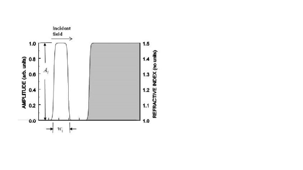
Figure 1: Representation of the field in the vacuum, in terms of the envelope of the vector potential, at some initial time $t=t_{0}$ before entering the dielectric. The field, on the left, is traveling to the right. The dielectric, draped with a gradient-index anti-reflection coating, is represented by the outline of the refractive index on the right.

According to the Maxwellian continuum electrodynamic theory, the nominal width of the pulse in the dielectric is the width of the incident pulse reduced by a factor of $n$ due to the reduced speed of light in a dielectric. The numerical solution of the wave equation confirms this theoretical fact.

The Minkowski electromagnetic energy formula is

$$U_{M}=\int_{\Sigma}{\sf T}_{M}^{00}\phi dz=\int_{\Sigma}\frac{n^{2}{\bf E}^{2}+{\bf B}^{2}}{2}dv\,.$$ (66)

Substituting the relations between the fields and vector potential into the energy formula, on obtains

$$\int_{\Sigma}|{\bf A}_{0}(t_{0},z)|^{2}\phi dz=\int_{\Sigma}n^{2}|{\bf A}_{0}(t_{1},z)|^{2}\phi dz\,,$$ (67)

where $\phi$ is the cross-sectional area of the field and comparisons have a per unit of cross-sectional area basis. This result is confirmed by numerical integration of the incident and refracted fields shown in Figs. 1 and 2. Using the fact that the width of the pulse is narrower in the medium by a factor of $n$ in Eq. (67), one finds, by energy conservation, that the amplitude of the vector potential in the dielectic is smaller than the incident vector potential amplitude by a factor of $\sqrt{n}$. This is confirmed in the numerical solution of the wave equation by an examination of Figs. 1 and 2. Both theoretically and numerically it is shown that the amplitude of the vector potential in the dielectric is the amplitude of the incident vector potential divided by $\sqrt{n}$. Applying this result to Eqs. (64) and (65), one finds that the amplitude of the electric field in the dielectric, $|{\bf E}_{0}|_{diel}$, is a factor of $\sqrt{n}$ smaller than the amplitude of the electric field that is incident from the vacuum, $|{\bf E}_{0}|_{inc}$. Meanwhile, the amplitude of the magnetic field in the dielectric is increased by a factor of $\sqrt{n}$ from the amplitude of the incident field. For a quasimonochromatic field in the quasistationary limit,

$$|{\bf E}_{0}|_{diel}=|{\bf E}_{0}|_{inc}/\sqrt{n}$$ (68a)

$$|{\bf B}_{0}|_{diel}=\sqrt{n}|{\bf B}_{0}|_{inc}\,.$$ (68b)

Applying the relations between the incident fields and the fields in the dielectric, Eqs. (68b), we find that ${\bf E}\times{\bf B}$ has a constant amplitude across the antireflection-coated entry face of the dielectric. Then, ${\bf E}\times{\bf B}$ is multiplied by $n^{2}/c$ to get the Minkowski momentum density. The pulse is narrower in the dielectric than in the vacuum by a factor of $n$ due to the reduced velocity of light in the dielectric. Substituting the relations between the incident fields and the fields in the dielectric into the Minkowski electromagnetic momentum formula

$${\bf G}_{M}=\frac{1}{c}\int_{\Sigma}\left({\sf T}_{M}^{10},{\sf T}_{M}^{20},{\sf T}_{M}^{30}\right)\phi dz=\int_{\Sigma}\frac{n^{2}{\bf E}\times{\bf B}}{c}dv$$ (69)

and comparing the results with Eqs. (66) and (67), we find that the Minkowski electromagnetic energy is constant in time but the Minkowski electromagnetic momentum is greater than the incident momentum by a factor of $n$ strongly violating the global conservation condition, Eq. (48). It could not be otherwise because Eqs. (66) and (69) have the same quadratic dependence of the fields but differ by a factor of $n$ in magnitude. Consequently, ${\bf G}_{M}(t_{1})$ is very different from the incident momentum and ${\sf T}_{M}^{\alpha\beta}$ is not an approximation of the total energy–momentum tensor, contrary to the conservation implied by Eq. (62) and contrary to statements in the scientific literature BIPfei ; BIObuk .

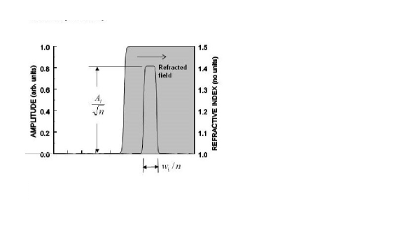
Figure 2: Representation of the field, in terms of the envelope of the vector potential, at a time $t=t_{1}$ when the field is entirely within the dielectric.

We have shown that energy–momentum relations that are systematically derived from the field equations using Maxwellian continuum electrodynamics are inconsistent with spacetime conservation laws if the gradient force is negligible as in Eq. (62). In order to avoid that fate, it has been the practice to make a physically motivated assumption that the macroscopic Maxwell–Minkowski equations describe an electromagnetic subsystem that is coupled to a material subsystem. We now examine this alternative, generally accepted as correct case BIRL ; BIBrev ; BIAMC3 ; BIKemplatest ; BIPfei ; BIAMC2 ; BIAMC4 ; BIAMC5 ; BIObuk ; BIObuk2 ; BIMuka ; BIMuka2 ; BIBarn ; BIPeierls ; BIBalazs ; BIGord ; BIMol ; BIBahder ; BIJMP , and show that it also leads to strong violation of spacetime conservation laws.

For a given electromagnetic energy–momentum four-tensor ${\sf T}_{em}^{\alpha\beta}$ (Minkowski, Abraham, etc.) there is an associated four-force density $f^{\alpha}_{em}$ such that

$$\partial_{\beta}{\sf T}_{em}^{\alpha\beta}=f^{\alpha}_{em}\,.$$ (70)

According to the current Abraham–Minkowski resolution theory BIRL ; BIBrev ; BIAMC3 ; BIKemplatest ; BIPfei ; BIAMC2 ; BIAMC4 ; BIAMC5 ; BIObuk ; BIObuk2 ; BIMuka ; BIMuka2 ; BIBarn ; BIPeierls ; BIBalazs ; BIGord ; BIMol ; BIBahder ; BIJMP , the dynamics of the material sub-system are based on a material four-tensor ${\sf T}_{matl}^{\alpha\beta}$ such that

$$\partial_{\beta}{\sf T}_{matl}^{\alpha\beta}=-f^{\alpha}_{em}\,.$$ (71)

We add Eqs. (70) and (71). Then the total energy–momentum tensor

$${\sf T}_{total}^{\alpha\beta}={\sf T}_{em}^{\alpha\beta}+{\sf T}_{matl}^{\alpha\beta}$$ (72)

obeys the local conservation law BIGiu

$$\partial_{\beta}{\sf T}_{total}^{\alpha\beta}=0$$ (73)

in accordance with the spacetime conservation law Eq. (47).

A wide variety of physical models have been employed in an effort to fully resolve the problem of momentum conservation in a dielectric BIRL ; BIBrev ; BIAMC3 ; BIKemplatest ; BIPfei ; BIAMC2 ; BIAMC4 ; BIAMC5 ; BIObuk ; BIObuk2 ; BIMuka ; BIMuka2 ; BIBarn ; BIPeierls ; BIBalazs ; BIGord ; BIMol ; BIBahder ; BIJMP . Selected examples are discussed in the next subsection. Typically, one assumes a microscopic model of the material dynamics in a dielectric and applies an averaging technique to derive the macroscopic momentum of the material. The correctness of the results is assumed to be affirmed by the fundamental nature of the physical laws that are used as the basis of the analysis. Adding the electromagnetic and material tensors, one obtains the total energy–momentum tensor for the thermodynamically closed system, Eq. (72). The total linear momentum

$${\bf G}_{total}=\frac{1}{c}\int_{\Sigma}\left({\sf T}_{total}^{10},{\sf T}_{total}^{20},{\sf T}_{total}^{30}\right)\phi dz=\int_{\Sigma}\frac{n{\bf E}\times{\bf B}}{c}dv$$ (74)

and the total energy

$$U_{total}=\int_{\Sigma}{\sf T}_{total}^{00}\phi dz=\int_{\Sigma}\frac{n^{2}{\bf E}^{2}+{\bf B}^{2}}{2}dv$$ (75)

are known quantities that can be related to the energy and momentum of the incident field in the vacuum because they are required to be constant in time by global conservation laws in the complete and closed system (unless one assumes inappropriate system boundaries). Using the corresponding total energy and total momentum densities to populate the total energy–momentum tensor, we write BIJMP

$${\sf T}_{total}^{\alpha\beta}\!=\!$$

$$\left[\begin{matrix}\frac{1}{2}(n^{2}{\bf E}^{2}+{\bf B}^{2})\!&(n{\bf E}\times{\bf B})_{1}\!&(n{\bf E}\times{\bf B})_{2}\!&(n{\bf E}\times{\bf B})_{3}\cr(n{\bf E}\times{\bf B})_{1}&{{\sf W}_{M}}_{11}&{{\sf W}_{M}}_{12}&{{\sf W}_{M}}_{13}\cr(n{\bf E}\times{\bf B})_{2}&{{\sf W}_{M}}_{21}&{{\sf W}_{M}}_{22}&{{\sf W}_{M}}_{23}\cr(n{\bf E}\times{\bf B})_{3}&{{\sf W}_{M}}_{31}&{{\sf W}_{M}}_{32}&{{\sf W}_{M}}_{33}\cr\end{matrix}\right]\,.$$ (76)

The total energy–momentum tensor, Eq. (76), is diagonally symmetric and traceless. Both the total energy, Eq. (75) and the total linear momentum, Eq. (74), are constant in time thereby satisfying the global conservation condition, Eq. (48). Applying the local conservation condition, Eq. (47), to the total energy–momentum tensor, Eq. (76), we find that the energy continuity equation

$$\frac{1}{c}\frac{\partial}{\partial t}\frac{1}{2}\left(n^{2}{\bf E}^{2}+{\bf B}^{2}\right)+\nabla\cdot(n{\bf E}\times{\bf B})=0$$ (77)

that is obtained for $\alpha=0$ is manifestly false because the two non-zero terms depend on different powers of $n$ in addition to being incommensurate with the Poynting theorem. This result is based on the total (electromagnetic plus material) energy–momentum tensor, Eq. (76), and is therefore independent of the particular electromagnetic representation, Abraham, Minkowski, etc., that is used. Then, the macroscopic Maxwell field equations and the spacetime conservation laws are laws of physics that are proven to be contradictory in the case of a thermodynamically closed system consisting of an electromagnetic subsystem and a dielectric material subsystem BIBrevnew . Clearly, the prescribed method to resolve the Abraham–Minkowski momentum dilemma produces only another contradiction.

It may be argued that pure induction without experimental support is not a method of theoretical physics. In our case, the energy–momentum evolution equations, Eqs. (32) and (38), are derived by formal theory directly from the laws of Maxwell-Minkowski continuum electrodynamics. Then the Minkowski momentum was shown to strongly violate global conservation laws. When these theorems are “fixed” by the addition of a physically motivated, but hypothetical, material energy–momentum tensor as shown in Eq. (72), the contrived total energy–momentum tensor, Eq. (76), leads to violation of other conditions of the spacetime conservation laws as shown by Eq. (77).

Proof by mathematical contradiction is far stronger than an experimental demonstration. One might recall that the 1887 Michelson–Morley experiment BIMichMor was initially interpreted to prove the existence of ether drag and was later deemed to support the absence of ether in the Einstein relativity theory. Likewise, the experiments that were originally viewed as support for the Abraham energy–momentum theory or the Minkowski theory, or both, will be shown in Sec. 7 to provide experimental justification for the new theory that is derived in Sec. 5.

IV.3 Brief Survey of Prior Work

The century-long history of the Abraham–Minkowski controversy BIMin ; BIAbr ; BIRL ; BIBrev ; BIAMC3 ; BIKemplatest ; BIPfei ; BIAMC2 ; BIAMC4 ; BIAMC5 ; BIObuk ; BIObuk2 ; BIMuka ; BIMuka2 ; BIBarn ; BIPeierls ; BIBalazs ; BIGord ; BIMol ; BIBahder ; BIJMP is a search for some provable description of momentum and momentum conservation for electromagnetic fields in dielectric media. A wide variety of physical principles have been applied to establish the priority of one type of momentum over another, or to establish that the Abraham and Minkowski formulations are equally valid. The modern resolution of the Abraham–Minkowski momentum controversy is to adopt a scientific conformity in which the Minkowski momentum and the Abraham momentum are both correct forms of electromagnetic momentum with the understanding that neither is the total momentum BIPfei ; BIAMC2 ; BIAMC5 ; BIBarn . Either the Minkowski momentum or the Abraham momentum can be used as the momentum of the electromagnetic field as long as that momentum is accompanied by the appropriate material momentum BIPfei . The material momentum is specific to a particular material and we will consider several well-known models that have appeared in the scientific literature in order to circumscribe the area of difficulty.

In a quasi-microscopic approach, the material momentum is often modeled as the aggregated kinematic momentum of individual particles of matter in the continuum limit. The total energy–momentum tensor is the sum of the electromagnetic energy–momentum tensor and the material energy–momentum tensor. In one example, Pfeifer, Nieminen, Heckenberg, and Rubinsztein-Dunlop BIPfei , posit that the total energy–momentum tensor is the sum of the Abraham energy–momentum tensor, Eq. (39), and the dust energy–momentum tensor

$${\sf T}_{mat,Abr}^{\alpha\beta}={\sf T}_{dust}^{\alpha\beta}=\left[\begin{matrix}\rho_{0}c^{2}\!&\rho_{0}cv_{1}\!&\rho_{0}cv_{2}\!&\rho_{0}cv_{3}\cr\rho_{0}cv_{1}&\rho_{0}v_{1}v_{1}&\rho_{0}v_{1}v_{2}&\rho_{0}v_{1}v_{3}\cr\rho_{0}cv_{2}&\rho_{0}v_{2}v_{1}&\rho_{0}v_{2}v_{2}&\rho_{0}v_{2}v_{3}\cr\rho_{0}cv_{3}&\rho_{0}v_{3}v_{1}&\rho_{0}v_{3}v_{2}&\rho_{0}v_{3}v_{3}\cr\end{matrix}\right]\,.$$ (78)

Here, $\rho_{0}$ is a constant mass density and ${\bf v}({\bf r},t)$ is a velocity field. The dust tensor, Eq. (78), is usually applied to a thermodynamically closed system consisting of non-interacting, neutral, mass-bearing particles in an inviscid, incoherent, unimpeded flow such that

$$\partial_{\beta}{\sf T}_{dust}^{\alpha\beta}=0$$ (79)

in the continuum limit. In the current context, however, the total tensor energy–momentum continuity equation is posited as BIPfei

$$\partial_{\beta}{\sf T}_{total}=\partial_{\beta}\left({\sf T}_{A}^{\alpha\beta}+{\sf T}_{dust}^{\alpha\beta}\right)=0\,.$$ (80)

Clearly, it is intended that the dust tensor is coupled to the Abraham electromagnetic tensor through the Abraham force density such that BIBethune

$$\partial_{\beta}{\sf T}_{dust}^{\alpha\beta}=-f^{\alpha}_{A}\,.$$ (81)

Performing the substitution of the dust tensor, Eq. (78), and the Abraham energy–momentum tensor, Eq. (39), into Eq. (80) results in BIPfei

$$\frac{1}{c}\frac{\partial}{\partial t}\left[\rho_{0}c^{2}+\frac{1}{2}\left(n^{2}{\bf E}^{2}+{\bf B}^{2}\right)\right]+\nabla\cdot(\rho_{0}{\bf v})+\nabla\cdot({\bf E}\times{\bf B})=0$$ (82)

for the $\alpha=0$ component of the total tensor energy–momentum continuity equation, Eq. (80). Because this sub-section is devoted to documenting the prior work, any issue with Eq. (82) does not condemn the new work that is presented in Secs. 5–7 of this article. Within the context of the prior work, Eq. (82) and, by extension, Eq. (97), are proven false in the next paragraph.

Pfeifer, Nieminen, Heckenberg, and Rubinsztein-Dunlop BIPfei then use global conservation of momentum arguments to phenomenologically relate the material momentum density to the electromagnetic momentum density with the ansatz

$$\rho_{0}{\bf v}={\bf g}_{total}-{\bf g}_{A}=(n-1)\frac{{\bf E}\times{\bf B}}{c}\,.$$ (83)

Substituting Eq. (83) into Eq. (82) produces BIPfei

$$\frac{1}{c}\frac{\partial}{\partial t}\left[\rho_{0}c^{2}+\frac{1}{2}\left(n^{2}{\bf E}^{2}+{\bf B}^{2}\right)\right]+\nabla\cdot(n{\bf E}\times{\bf B})=0\,.$$ (84)

The total energy and total momentum are both quadratic in the fields and must have the same dependence on the refractive index $n$. We note that if the particle density $\rho_{0}$ is constant then Eq. (84) reproduces Eq. (77) and is manifestly false because the two nonzero terms would depend on different powers of the refractive index and because the equation would be incommensurate with Poynting’s theorem. Although Pfeifer, Nieminen, Heckenberg, and Rubinsztein-Dunlop BIPfei do not propose a time-dependent model for the particle density $\rho_{0}$, the two non-zero terms of the energy continuity equation will be incommensurate unless Eq. (84) becomes

$$\frac{n}{c}\frac{\partial}{\partial t}\left[\frac{1}{2}\left(n^{2}{\bf E}^{2}+{\bf B}^{2}\right)\right]+\nabla\cdot(n{\bf E}\times{\bf B})=0\,.$$ (85)

The corresponding tensor continuity equation for the total energy and the total momentum

$$\bar{\partial}_{\beta}{\sf T}_{total}^{\alpha\beta}=0$$ (86)

is false because the presence of the index-dependent material four-divergence operator BIFinn ; BIJMP

$$\bar{\partial}_{\beta}=\left(\frac{n}{c}\frac{\partial}{\partial t},\frac{\partial}{\partial x},\frac{\partial}{\partial y},\frac{\partial}{\partial z}\right),$$ (87)

violates the conservation condition, Eq. (73), for $\alpha=0$. This result shows that the total energy and the total momentum being constant in time does not guarantee that the evolution equations for the total energy and the total momentum satisfy the local conservation law, in fact, just the opposite.

In an influential 1973 article, Gordon BIGord uses a microscopic model of the dielectric in terms of electric dipoles. Assuming a dilute vapor in which the dipoles do not interact with each other or their host, Gordon writes the microscopic Lorentz dipole force on a particle with linear polarizability $\alpha$ as BIAMC3 ; BIGord ; BIPenHaus

$${\bf f}_{atom}=\alpha\left(({\bf e}\cdot\nabla){\bf e}+\frac{d{\bf e}}{dt}\times{\bf b}\right)$$ (88)

in the vacuum, where ${\bf e}$ is the microscopic electric field and ${\bf b}$ is the microscopic magnetic field. The material momentum density is obtained by spatially averaging the force on a single dipole and integrating with respect to time. Then the material momentum density is

$${\bf g}_{matl}=\int\langle N{\bf f}_{atom}\rangle dt\,,$$ (89)

where $N$ is the dipole density. The fields acting on the dipoles inside a dielectric are not the same as the fields in free space. For the purpose of presenting the prior work, we suffer, without proof, that the material momentum density is BIGord

$${\bf g}_{matl}=N\alpha\int\frac{{\bf E}\times{\bf B}}{c}dt+N\alpha\int\frac{1}{2}\nabla({\bf E}^{2})dt\,.$$ (90)

Gordon assumes that the total momentum density is the sum of the Abraham momentum density and the material momentum density. Making a transformation to retarded time BIIcsevgiLamb , Gordon BIGord derives

$${\bf g}_{G}=\frac{n{\bf E}\times{\bf B}}{c}$$ (91)

for the total momentum density and then assumes a pseudo-momentum in order to force agreement with the Minkowski form of momentum.

In the Gordon model, and similar models, the dipoles are free particles in the vacuum that are accelerated by the Lorentz dipole force at the leading edge of the quasi-monochromatic field and travel at constant velocity until decelerated by the Lorentz dipole force at the trailing edge of the field. In a real dielectric, or a more complete theoretical model of a dielectric, the motion of the material dipoles will be considerably impeded by collisions, lattice strains, or other effects of the host material. Consequently, it is assumed that a traveling deformation of the material, rather than the unrestrained motion of dipoles, will contribute the requisite material momentum BIPfei ; BIGord . The Gordon linear momentum

$${\bf G}_{G}=\int_{\Sigma}{\bf g}_{G}dv=\int_{\Sigma}\frac{n{\bf E}\times{\bf B}}{c}dv$$ (92)

that is obtained by spatially integrating the Gordon momentum density and the Minkowski momentum, Eq. (69), that is obtained by adding a hypothetical pseudomomentum concludes the derivation. Comparing Eq. (92) to Eq. (66), the Gordon momentum ${\bf G}_{G}$ is constant in time in the case of propagation of a quasimonochromatic field through a gradient-index antireflection-coated simple linear dielectric BIBahder ; BIJMP ; BIGord . Then, we now have a plausible model for the material momentum.

There are several problems with the derivation presented in Ref. BIGord in addition to the assumptions that are described above: i) In Eq. (88), the force density $\alpha({\bf e}\cdot\nabla){\bf e}$ has been improperly retained because several other terms of the same order have been dropped in the dipole approximation BICrendrr . Moreover, this small term is divided into two large terms of nearly equal magnitude and opposite sign and one of these terms is eliminated. ii) Temporal independence of the total linear momentum is only one of the four conditions of the energy–momentum conservation laws, Eqs. (47)–(50). iii) There is a factor of 2 error in the susceptibility used by Gordon. In the corrected version of the Gordon derivation, Milonni and Boyd BIAMC3 prove that the sum of the electromagnetic and material momentums is the Minkowski momentum, Eq. (2), which is not constant in time.

Barnett and Loudon BIAMC2 and Barnett BIBarn present a model in which the Abraham momentum and the Minkowski momentum are both appropriate momentums for the field in a dielectric. Each of the classical electromagnetic momentums is accompanied by a material momentum, different in each case, and identified with either a canonical or kinetic phenomenology. The material momentum densities, ${\bf g}_{canonical}^{matl}$ and ${\bf g}_{kinetic}^{matl}$, are defined implicitly by global conservation of total momentum, such that

$${\bf G}_{total}={\bf G}_{M}+\int_{\Sigma}{\bf g}_{canonical}^{matl}dv={\bf G}_{A}+\int_{\Sigma}{\bf g}_{kinetic}^{matl}dv\,,$$ (93)

where ${\bf G}_{total}={\bf G}_{incident}$ for a gradient-index anti-reflection coated simple linear dielectric block. Although providing a descriptive model for construction of the total linear momentum, the total linear momentum, ${\bf G}_{total}$, is unique in a thermodynamically closed system because it is constant in time and it is a known quantity in terms of macroscopic fields, Eq. (74). As in the previous example, temporal independence of the total linear momentum is only one of the four conditions of the spacetime conservation laws, Eqs. (47)–(50). If we use either of the canonical or kinetic models of Eq. (93) for the total linear momentum, then the total energy–momentum tensor will be the same as Eq. (76). Applying the local conservation condition, Eq. (73), the four-divergence of the total energy–momentum tensor will produce a demonstrably false energy continuity equation, just as before, Eq. (77). Again, the two nonzero terms in Eq. (77) depend on different powers of the refractive index and Eq. (77) is incommensurate with the Poynting theorem.

Ramos, Rubilar, and Obukhov BIObuk utilize a fully relativistic 4-dimensional tensor formalism to discuss the energy–momentum of a system that consists of an antireflection-coated rigid slab of dielectric with a final constant velocity ${\bf v}$. Their total energy–momentum tensor is

$${\sf T}_{\mu}^{\;\;\nu}=\rho_{0}u_{\mu}u^{\nu}+\Big{(}{\sf F}_{\mu\sigma}F^{\sigma\nu}+\frac{1}{4}\delta_{\mu}^{\nu}F^{\sigma\lambda}{\sf F}_{\sigma\lambda}\Big{)}$$

$$+(n^{2}-1)\Big{(}{\sf F}_{\mu\sigma}F^{\lambda\nu}u^{\sigma}u_{\lambda}+\frac{1}{2}\delta_{\mu}^{\nu}{\sf F}_{\sigma\rho_{0}}F^{\sigma\lambda}u^{\rho_{0}}u_{\lambda}$$

$$-F^{\rho_{0}\sigma}{\sf F}_{\rho_{0}\lambda}u_{\sigma}u^{\lambda}u_{\mu}u^{\nu}\Big{)}\,,$$ (94)

where $u^{\mu}$ is the four-velocity $(\gamma,\gamma{\bf v})$. Ramos, Rubilar, and Obukhov BIObuk claim that the total energy–momentum tensor, Eq. (94), satisfies the energy–momentum balance equation

$$\partial_{\nu}{\sf T}_{\mu}^{\;\;\nu}-{\sf F}_{\mu\nu}J^{\nu}_{ext}=0\,,$$ (95)

that the energy–momentum tensor of the complete system is conserved, and that the system is thermodynamically closed if the four-current density $J^{\nu}_{ext}$ is zero. Then the total four-momentum of the whole system is globally conserved and

$$P_{j}=\int_{\Sigma}{\sf T}_{j}^{\;\;0}dv$$ (96)

is a time-independent quantity BIObuk . In order to test the validity of the total energy–momentum tensor, Eq. (94), we consider a quasimonochromatic field in the plane-wave limit to be normally incident on a simple linear dielectric through a gradient-index antireflection coating. Evaluating the $\nu=0$ element of Eq. (95), we obtain

$$\frac{\partial}{\partial(ct)}\left[\rho_{0}c^{2}+\frac{1}{2}(n^{2}{\bf E}^{2}+{\bf B}^{2})\right]+\nabla\cdot(\rho_{0}{\bf v})+\nabla\cdot({\bf E}\times{\bf B})=0$$ (97)

by substitution from the total energy–momentum tensor, Eq. (94), using quantities from the usual antisymmetric field tensor

$${\sf F}^{\alpha\beta}=\left[\begin{matrix}0\!&-E_{x}\!&-E_{y}\!&-E_{z}\cr E_{x}&0&-B_{z}&B_{y}\cr E_{y}&B_{z}&0&-B_{x}\cr E_{z}&-B_{y}&B_{x}&0\cr\end{matrix}\right]\,.$$ (98)

Now, Eq. (97) is the same as Eq. (82) that was derived previously using the model of Pfeifer, Nieminen, Heckenberg, and Rubinsztein-Dunlop BIPfei . Substituting Eq. (83) into Eq. (97) and taking $\rho_{0}$ as constant in time BIObuk , we write

$$\frac{1}{c}\frac{\partial}{\partial t}\left[\frac{1}{2}\left(n^{2}{\bf E}^{2}+{\bf B}^{2}\right)\right]+\nabla\cdot\left(n{\bf E}\times{\bf B}\right)=0\,.$$ (99)

As before, Eq. (99) i) is incommensurate with the Poynting theorem and ii) is self-inconsistent because the two non-zero terms depend on different powers of the refractive index thereby disproving the energy–momentum balance equation, Eq. (95), with $J^{\nu}_{ext}=0$.

A fully microscopic model of the interaction of light with ponderable matter is unique, valid, and beyond our capabilities. The examples above are representative of the many diverse quasi-microscopic treatments of the Abraham–Minkowski controversy and there is no unique quasi-microscopic model BIPfei . There are many ways to couple and average the quasi-microscopic material properties with the electromagnetic properties that are systematically derived from the macroscopic Maxwell–Minkowski equations. The correctness of the procedure is rooted in the fundamental basis of the model and the derivation. In the end, the total linear momentum is the sum of the electromagnetic momentum and the material momentum. However, the spacetime conservation laws are not satisfied. We provided specific examples, using the models of Pfeifer, Nieminen, Heckenberg, and Rubinsztein-Dunlop BIPfei , of Barnett BIBarn , and of Ramos, Rubilar, and Obukhov BIObuk , where the continuity equation for the total energy is proven to be false. More importantly, these are general results as shown in Sec. 4B. Any construction of the total energy–momentum tensor must be based on energy and momentum densities corresponding to the time independent total energy, Eq. (75) and the time independent total momentum, Eq. (74). Then the four-divergence of the total energy–momentum tensor that is constructed using Maxwellian continuum electrodynamics will always result in a provably false energy continuity equation, even if a phenomenological material energy–momentum tensor is assumed.

V Lagrangian Field Dynamics in a Dielectric-Filled Spacetime

At the fundamental microscopic level, dielectrics consist of tiny bits of host and polarizable matter, embedded in the vacuum, with interactions of various types. According to Lorentz, the seat of the electromagnetic field is empty space. If a light pulse is emitted from a point $(x_{a},y_{a},z_{a})$ at time $t_{a}$ then spherical wavefronts are defined by

$$(x-x_{a})^{2}+(y-y_{a})^{2}+(z-z_{a})^{2}=\left(c(t-t_{a})\right)^{2}$$ (100)

in a flat four-dimensional Minkowski spacetime $S_{v}(ct,x,y,z)$. Equation (100) underlies classical electrodynamics and its relationship to special relativity. Although light always travels at speed $c$ BIFeynman , Eq. (100) is only valid at very short range before the light is scattered by the various microscopic features of the dielectric. While the microscopic picture is always valid, there are practical difficulties in treating all of the interactions as light traverses a dielectric.

In continuum electrodynamics, the dielectric is treated as continuous at all length scales and the macroscopic refractive index $n$ is defined such that light travels with an effective speed of $c/n$. In an arbitrarily large simple linear dielectric medium with an isotropic homogeneous index of refraction $n$, spherical wavefronts from a point source at $(x_{a},y_{a},z_{a})$ and emitted at time $t_{a}$ are defined by

$$(x-x_{a})^{2}+(y-y_{a})^{2}+(z-z_{a})^{2}=\left(\frac{c(t-t_{a})}{n}\right)^{2}\,.$$ (101)

At this point, we postulate Eq. (101), instead of Eq. (100), as the basis of a theory of continuum electrodynamics and derive the consequences for field theory, classical continuum electrodynamics, special relativity, spacetime, and experiments.

We consider an arbitrarily large region of space to be filled with a simple linear isotropic homogeneous dielectric that is characterized by a linear refractive index $n$. For clarity and concision, we will work in a regime in which dispersion can be treated parametrically and is otherwise negligible such that $n(\omega_{p})$ is a real time-independent constant for a transparent dielectric that is illuminated by a quasimonochromatic field of center frequency $\omega_{p}$, as described in Sec. 2. We define an inertial reference frame $S(x,y,z)$ with orthogonal axes, $x$, $y$, and $z$, and require that the origin of the reference frame is significantly inside the volume that is defined by the surface of the dielectric medium. We denote a time-like coordinate in the medium as $\bar{x}_{0}$. If a light pulse is emitted from the origin at time

$$\tau=\bar{x}_{0}/c=0\,,$$ (102)

then

$$x^{2}+y^{2}+z^{2}=\left(\bar{x}_{0}\right)^{2}$$ (103)

describes spherical wavefronts in $S$. The four-vector $(\bar{x}_{0},x,y,z)$ represents the position of a point in a four-dimensional, isotropic, homogeneous, flat, non-Minkowski material spacetime $S_{d}(\bar{x}_{0},x,y,z)$. Clearly, the new time-like coordinate $\bar{x}_{0}$ is associated with $c\tau=ct/n$, while $x_{0}=ct$ is the usual time-like coordinate in a vacuum Minkowski spacetime. The material spacetime reduces to ordinary Minkowski spacetime if $n=1$.

The basis functions, $\exp(-i(n\omega/c)(\bar{x}_{0}-{\bf\hat{k}}_{0}\cdot{\bf r}))$, define the null surface, $\bar{x}_{0}={\bf\hat{k}}_{0}\cdot{\bf r}$. Fig. 3 is a depiction of the intersection of the light cone with the $x-\bar{x}_{0}$ plane in the flat material spacetime $S_{d}$ showing the null $\bar{x}_{0}=x$. There will be a different material spacetime for each value of the refractive index, but the half-opening angle of the material light cone will always be $\alpha=\pi/4$ in the corresponding material spacetime. The unit slope of the null in the $x-\bar{x}_{0}$ plane of the non-Minkowski material spacetime is related to the coordinate speed of light in a simple linear dielectric by

$$\frac{\Delta x}{\Delta t}=\frac{\Delta x}{\Delta\bar{x}_{0}}\frac{d\bar{x}_{0}}{dt}=1\cdot\frac{c}{n}=\frac{c}{n}\,.$$ (104)

This equation shows that the effective speed of light in a simple linear dielectric medium is attributable to renormalization of the time-like coordinate by $n$.

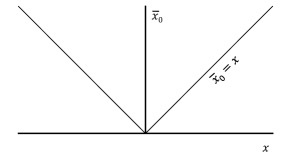
Figure 3: Null cone for light depicted in the $\bar{x}_{0}-x$ plane of a flat, non-Minkowski material spacetime that corresponds to a simple linear dielectric.

For a system of particles, the transformation of the position vector ${\bf x}_{i}$ of the $i^{th}$ particle to $J$ independent generalized coordinates is

$${\bf x}_{i}={\bf x}_{i}(\tau;q_{1},q_{2},\ldots,q_{J}).$$ (105)

Applying the chain rule, we obtain the virtual displacement

$$\delta{\bf x}_{i}=\sum_{j=1}^{J}\frac{\partial{\bf x}_{i}}{\partial q_{j}}\delta q_{j}$$ (106)

and the velocity

$${\bf u}_{i}=\frac{d{\bf x}_{i}}{d\tau}=\sum_{j=1}^{J}\frac{\partial{\bf x}_{i}}{\partial q_{j}}\frac{dq_{j}}{d\tau}+\frac{\partial{\bf x}_{i}}{\partial\tau}$$ (107)

of the $i^{th}$ particle in the new coordinate system. Substitution of

$$\frac{\partial{\bf u}_{i}}{\partial(dq_{j}/d\tau)}=\frac{\partial{\bf x}_{i}}{\partial q_{j}}$$ (108)

into the identity

$$\frac{d}{d\tau}\left(m{\bf u}_{i}\cdot\frac{\partial{\bf x}_{i}}{\partial q_{j}}\right)=m\frac{d{\bf u}_{i}}{d\tau}\cdot\frac{\partial{\bf x}_{i}}{\partial q_{j}}+m{\bf u}_{i}\cdot\frac{d}{d\tau}\left(\frac{\partial{\bf x}_{i}}{\partial q_{j}}\right)$$ (109)

yields

$$\frac{d{\bf p}_{i}}{d\tau}\cdot\frac{\partial{\bf x}_{i}}{\partial q_{j}}=\frac{d}{d\tau}\left(\frac{\partial}{\partial(dq_{j}/d\tau)}\frac{1}{2}m{\bf u}_{i}^{2}\right)-\frac{\partial}{\partial q_{j}}\left(\frac{1}{2}m{\bf u}_{i}^{2}\right).$$ (110)

For a system of particles in equilibrium, the virtual work of the applied forces ${\bf f}_{i}$ vanishes and the virtual work on each particle vanishes leading to the principle of virtual work

$$\sum_{i}{\bf f}_{i}\cdot\delta{\bf x}_{i}=0$$ (111)

and D’Alembert’s principle

$$\sum_{i}\left({\bf f}_{i}-\frac{d{\bf p}_{i}}{d\tau}\right)\cdot\delta{\bf x}_{i}=0.$$ (112)

Using Eqs. (106) and (110) and the kinetic energy of the $i^{th}$ particle

$${T}_{i}=\frac{1}{2}m{\bf u}_{i}^{2},$$ (113)

we can write D’Alembert’s principle, Eq. (112), as

$$\sum_{j}^{J}\left[\left(\frac{d}{d\tau}\left(\frac{\partial T}{\partial(dq_{j}/d\tau)}\right)-\frac{\partial T}{\partial q_{j}}\right)-Q_{j}\right]\delta q_{j}=0$$ (114)

in terms of the generalized forces

$$Q_{j}=\sum_{i}{\bf f}_{i}\cdot\frac{\partial{\bf x}_{i}}{\partial q_{j}}.$$ (115)

If the generalized forces come from a generalized scalar potential function $V$ BIGold , then we can write Lagrange equations of motion

$$\frac{d}{d\tau}\left(\frac{\partial L}{\partial(\partial q_{j}/\partial\tau)}\right)-\frac{\partial L}{\partial q_{j}}=0,$$ (116)

where $L=T-V$ is the Lagrangian. The canonical momentum is therefore

$$p_{j}=\frac{\partial L}{\partial(\partial q_{j}/\partial\tau)}$$ (117)

in a linear medium. Comparable derivations for the vacuum case, $\tau\rightarrow t$, appear in Goldstein BIGold and Marion BIMar , for example. This version of canonical momentum differs from the existing vacuum formula because the material time $\tau$ appears instead of the vacuum time $t$.

The field theory BICT is based on a generalization of the discrete case in which the dynamics are derived from a Lagrangian density ${\cal L}$. The generalization of the Lagrange equation, Eq. (116), for fields in a linear medium is

$$\frac{d}{d\bar{x}_{0}}\frac{\partial{\cal L}}{\partial(\partial A_{j}/\partial\bar{x}_{0})}=\frac{\partial{\cal L}}{\partial A_{j}}-\sum_{i}\partial_{i}\frac{\partial{\cal L}}{\partial(\partial_{i}A_{j})}\,.$$ (118)

This equation differs from the Lagrange equation for fields in the vacuum BICT

$$\frac{d}{dx_{0}}\frac{\partial{\cal L}}{\partial(\partial A_{j}/\partial x_{0})}=\frac{\partial{\cal L}}{\partial A_{j}}-\sum_{i}\partial_{i}\frac{\partial{\cal L}}{\partial(\partial_{i}A_{j})}$$ (119)

in that differentiation is performed with respect to the material time-like coordinate $\bar{x}_{0}$ instead of the vacuum coordinate $x_{0}$. We take the Lagrangian density of the electromagnetic field in the medium to be

$${\cal L}=\frac{1}{2}\left(\left(\frac{\partial{\bf A}}{\partial\bar{x}_{0}}\right)^{2}-(\nabla\times{\bf A})^{2}\right)\,.$$ (120)

Again, differentiation is performed with respect to the material time-like coordinate $\bar{x}_{0}$ instead of the vacuum coordinate $x_{0}$. Furthermore, the Lagrangian density is explicitly quadratic in the macroscopic fields corresponding to real eigenvalues and a conservative system.

Equations (118) and (120) form the basis for a new canonical theory of macroscopic fields in a simple linear dielectric. The new theory has similarities in appearance to the macroscopic Maxwell equations, but it is disjoint from the Maxwell theory because it is based in a flat non-Minkowski material spacetime $S_{d}(\bar{x}_{0},x,y,z)$ instead of a vacuum Minkowski spacetime $S_{v}(x_{0},x,y,z)$. Constructing the components of Eq. (118), we have

$$\frac{\partial{\cal L}}{\partial(\partial A_{j}/\partial\bar{x}_{0})}=\frac{\partial A_{j}}{\partial\bar{x}_{0}}$$ (121)

$$\frac{\partial\cal L}{\partial A_{j}}=0$$ (122)

$$\sum_{i}\partial_{i}\frac{\partial{\cal L}}{\partial(\partial_{i}A_{j})}=[\nabla\times(\nabla\times{\bf A})]_{j}$$ (123)

for the Lagrangian density given in Eq. (120). We substitute the individual terms, Eqs. (121)–(123), into Eq. (118), then the Lagrange equations of motion for the electromagnetic field in a dielectric are the three orthogonal components of the vector wave equation

$$\nabla\times(\nabla\times{\bf A})+\frac{\partial^{2}{\bf A}}{\partial\bar{x}_{0}^{2}}=0\,.$$ (124)

For fields, the canonical momentum density

$$\Pi_{j}=\frac{\partial{\cal L}}{\partial(\partial A_{j}/\partial\bar{x}_{0})}$$ (125)

from Eq. (121) supplants the discrete canonical momentum defined in Eq. (117).

We can write the second-order equation, Eq. (124), as a set of first-order differential equations. To that end, we introduce macroscopic field variables

$${\bf\Pi}=\frac{\partial{\bf A}}{\partial\bar{x}_{0}}$$ (126)

$${\bf B}=\nabla\times{\bf A}.$$ (127)

Here, ${\bf\Pi}$ is the canonical momentum field density whose components were defined in Eq. (125) after making the substitutions indicated by Eq. (121). Substituting the definition of the canonical momentum field ${\bf\Pi}$, Eq. (126), and the definition of the magnetic field ${\bf B}$, Eq. (127), into Eq. (124), we obtain the Maxwell–Ampère-like law

$$\nabla\times{\bf B}+\frac{\partial{\bf\Pi}}{\partial\bar{x}_{0}}=0\,.$$ (128)

The divergence of Eq. (127) and the curl of Eq. (126) respectively produce Thompson’s Law

$$\nabla\cdot{\bf B}=0$$ (129)

and a Faraday-like law

$$\nabla\times{\bf\Pi}-\frac{\partial{\bf B}}{\partial\bar{x}_{0}}=\frac{\nabla n}{n}\times{\bf\Pi}\,.$$ (130)

The divergence of the variant Maxwell–Ampère Law, Eq. (128), is

$$\frac{\partial}{\partial\bar{x}_{0}}\nabla\cdot{\bf\Pi}=-\frac{\nabla n}{n}\cdot\frac{\partial{\bf\Pi}}{\partial\bar{x}_{0}}\,.$$ (131)

Integrating Eq. (131) with respect to the time-like coordinate yields a modified version of Gauss’s law

$$\nabla\cdot{\bf\Pi}=-\frac{\nabla n}{n}\cdot{\bf\Pi}-c_{1}$$ (132)

where $-c_{1}$ is a constant of integration. Based on the derivation of these equations, it is required that the source terms in Eqs. (130) and (132) that involve the gradient of the refractive index are, at most, perturbative, essentially limiting the theory to an isotropic homogeneous block of simple linear dielectric draped with a gradient-index antireflection coating or a piecewise homogeneous simple linear dielectric. We have not included free charges and a free-charge current because it is an unnecessary complication and because an inviscid incoherent flow of non-interacting charges in the continuum limit moving unimpeded through a continuous dielectric cannot be justified at the level of rigor that we are employing in the current work.

This completes the set of first-order equations of motion for the macroscopic fields, Eqs. (128)–(130) and (132). Consolidating the equations of motion and dropping the inhomogeneous source terms, we have the equations of motion for macroscopic electromagnetic fields in an isotropic homogeneous simple linear dielectric,

$$\nabla\times{\bf B}+\frac{\partial{\bf\Pi}}{\partial\bar{x}_{0}}=0$$ (133a)

$$\nabla\cdot{\bf B}=0$$ (133b)

$$\nabla\times{\bf\Pi}-\frac{\partial{\bf B}}{\partial\bar{x}_{0}}=0$$ (133c)

$$\nabla\cdot{\bf\Pi}=0\,,$$ (133d)

derived from field theory for quasimonochromatic electromagnetic fields in a linear dielectric-filled, flat, non-Minkowski continuous material spacetime.

Readers of this article may note that the macroscopic field equations, Eqs. (133d), obviously violate special relativity because ${\bar{x}}_{0}$ is index-dependent. It is also obvious that Eqs. (133d) cannot possibly violate special relativity because their form is isomorphic to an easily verified identity of the macroscopic Maxwell–Minkowski equations, Eqs. (6d), which are known to satisfy special relativity. Readers should not unequivocally, uncritically, and untenably advocate one side or the other of this contradiction based solely on the appearance of Eqs. (133d). It is shown in Ref. BIPrepr that Eqs. (133d) comply with Rosen dielectric special relativity. The applicability of the Fresnel relations to the system described by Eqs. (133d) has been questioned and treated in Ref. BIFresnel . Other issues like free charges, free charge currents, experimental verification, dispersion, plane-wave limit, material motion, etc. were addressed as they came up in the description.

We can never place a matter-based observer, no matter how small, in a continuous dielectric because the model dielectric is continuous at all length scales and will always be displaced. Consequently, the necessity to make non-optical measurements in a vacuum leads to the establishment of a Laboratory Frame of Reference. An observer that resides in the vacuum by virtue of displacing the terrestrial atmosphere outside of the dielectric, such as Fizeau BIFizeau , will measure the speed of light in a dielectric to be dependent on the velocity of the dielectric relative to the vacuum-based Laboratory Frame of Reference, Eq. (16), an effect that Fresnel attributed to ether drag.

In deriving the theory of dielectric special relativity, Laue considered a block of dielectric moving inertially in a Laboratory Frame of Reference and used the Einstein velocity sum rule to derive the theory of dielectric special relativity and confirm Fresnel drag. That physical configuration is not correct for the special relativity that underlies the equations of motion for electromagnetic fields in a dielectric, Eqs. (133d). The current author BIPrepr derived a theory of dielectric special relativity for inertial reference frames translating at constant speed in an arbitrarily large region of space in which the speed of light is $c/n$ in the local rest frame. This rigorous derivation of special relativity in an appropriate physical configuration confirms Rosen’s BIRosen phenomenological derivation of an index-dependent theory of special relativity in a dielectric. The speed of light at the location of the observer in the dielectric is obviously independent of the motion of the dielectric; otherwise there would be an inaccessible preferred Laboratory Reference Frame. The situation is different from the Laue theory; there the vacuum-based Laboratory Frame of Reference is established first and the motion of the dielectric in the preferred Laboratory Reference Frame can be specified and measured.

Rosen BIRosen noted that there will be a different theory of relativity associated with a limiting speed in each material. In the rest frame of the material, the speed of light $c_{d}$ will be different in different dielectric materials and we can label different materials with the index $i$. Considering only isotropic, homogeneous linear dielectric materials in which the speed of light is inversely proportional to a real constant $n_{i}$, we obtain

$$({\gamma_{d}})_{i}=\frac{1}{\sqrt{1-n_{i}^{2}v_{d}^{2}/c^{2}}}$$ (134)

as our material-specific Lorentz factor BIPrepr ; BIRosen . As discussed above, the configuration of the physical system that we are treating is different from the system that was employed by Laue BILaue ; BILaue2 .

In this article, the theory of quasimonochromatic radiation interacting with a simple linear dielectric has been discussed primarily in terms of an arbitrarily large isotropic homogeneous medium or a block of an isotropic, homogeneous, linear dielectric material draped with a gradient-index anti-reflection coating. At some point, we will be required to deal with the boundary conditions of piecewise homogeneous linear dielectric materials. Reflection and refraction are experimentally uncomplicated and it would be unpleasant if the usual Fresnel formulas failed to work for the new theory. On the other hand, it is apparent that the usual derivation of the Fresnel relations BIMar ; BIGriff ; BIJackson ; BIZangwill by application of the Stoke’s theorem and the divergence theorem to the Maxwell–Minkowski equations will not work when applied to the new field equations, Eqs. (133d). Boundary conditions and the Fresnel relations are rigorously derived by conservation of energy and the application of Stoke’s theorem to the wave equation in a separate publication BIFresnel .

We cannot rigorously relate the ordinary macroscopic Maxwell–Minkowski field equations, Eqs. (6d), to the results of our derivation, Eqs. (133d). In the current formalism, based on Lagrangian field theory adapted to a region of space in which the speed of light is $c/n$, the usual macroscopic Maxwell fields ${\bf E}$ and ${\bf D}$ are not definable in terms of ${\bf\Pi}$ because the refractive index is contained in the independent coordinate and is not a free material parameter. As disclosed by Rosen BIRosen , there is a different theory of relativity associated with each isotropic homogeneous medium in which a limiting speed is associated with the phenomena that take place in the medium. Likewise, there is a different theory of electrodynamics for each linear medium, labelled $i$, with refractive index $n_{i}$ and the different theories correspond to disjoint isotropic, homogeneous, flat, non-Minkowski material spacetimes BIRosen $(S_{d})_{i}(\bar{x}_{0_{ii}},x,y,z)$. Then the macroscopic Maxwell–Minkowski equations, Eqs. (6d), cannot be derived as valid theorems from our new axioms, Eqs. (133d), and we cannot insert, by hand, familiar expressions that were derived from Maxwellian continuum electrodynamics into the new theory.

Nevertheless, we would like to informally compare and contrast the new theory with Maxwellian continuum electrodynamics. There is sufficient commonality with the classic theories that simple phenomena like refraction and wave velocity have equivalent formulations in the new theory. Then, there are special cases in which the new {${\bf\Pi}$,${\bf B}$} continuum electrodynamics can be phenomenologically related to the usual Minkowski representation {${\bf E}$,${\bf B}$,${\bf D}$,${\bf H}$} of the macroscopic Maxwell equations. These typically involve situations in which only one of the equations of macroscopic electrodynamics is needed, such as the wave equation

$$\nabla\times(\nabla\times{\bf A})+\frac{\partial}{\partial\bar{x}_{0}}\left(\frac{\partial{\bf A}}{\partial\bar{x}_{0}}\right)=0$$ (135)

that is derived by substituting the definitions of the macroscopic fields, Eqs. (126) and (127), into the Maxwell–Ampère-like law, Eq. (133a). Therefore, we can be assured that the extensive theoretical and experimental work that is “correctly” described by the macroscopic Maxwell theory of continuum electrodynamics has an equivalent, or nearly equivalent, expression in the new theory. Nevertheless, we must be very careful about integrating established concepts and formulas of Maxwellian electrodynamics into the new version of continuum electrodynamics.

More interesting is the work that we can do with the new formalism of continuum electrodynamics that was improperly posed in the standard Maxwell theory of continuum electrodynamics. These cases will typically involve the invariance or tensor properties of the set of coupled equations of motion. This interpretation is borne out in our common experience: the macroscopic Maxwell–Minkowski equations produce exceedingly accurate experimentally verified predictions of simple phenomena like reflection, refraction, Fresnel relations, wave propagation, etc., but fail to render a unique, uncontroversial, experimentally verifiable prediction of energy–momentum conservation. In the next section, we will demonstrate the utility of the new formalism of continuum electrodynamics by addressing energy–momentum conservation in a dielectric.

VI Conservation Laws and $\{{\bf\Pi},{\bf B}\}$ Electrodynamics

The derivation of the continuity equation of a property flux density is described in Sec. 3 as applying the divergence theorem to a Taylor series expansion of the property density field $\rho$ and the property flux density field ${\bf g}=\rho{\bf u}$ to a continuous flow in an otherwise empty volume BIFox . Here, we are treating the continuous (continuum limit) flow of photons (light field) in an arbitrarily large, isotropic, homogeneous, simple linear dielectric that is modeled as a region of space in which the speed of light is $c/n$. Therefore, the conditions on the flow differ from the vacuum conditions that are assumed for the usual spacetime conservation laws that were discussed in Sec. 3. Microscopically, dielectrics are mostly empty space. But, in the continuum limit, dielectrics are continuous at all length scales and the light field cannot be treated as if it is flowing in an otherwise empty volume.

It is necessary to modify the spacetime conservation laws that were presented in Sec. 3 for the flow of a photon fluid (light field) in a non-empty volume. As shown in Eq. (105), the generalized temporal coordinate in a dielectric-filled volume is $\tau$. Then a continuity equation has the form

$$\frac{\partial\rho}{\partial\tau}+\nabla\cdot(\rho{\bf u})=0$$ (136)

in an arbitrarily large region of space that is filled with an isotropic, homogeneous, simple linear dielectric material.

We can compare the conservation laws in a dielectric-filled spacetime with the vacuum conservation laws Eqs. (47)–(50), in an empty volume.

1) Continuity equations in a dielectric have the form of Eq. (136), instead of Eq. (41). Writing a scalar continuity equation for energy and a scalar continuity equation for each of the three components of the momentum, row-wise, we obtain the differential equation

$$\bar{\partial}_{\beta}{\sf T}^{\alpha\beta}=0$$ (137)

instead of Eq. (43) as a condition for conservation of energy and momentum for a continuous unimpeded flow in a dielectric-filled spacetime. The material four-divergence operator

$$\bar{\partial}_{\beta}=\left(\frac{1}{c}\frac{\partial}{\partial\tau},\frac{\partial}{\partial x},\frac{\partial}{\partial y},\frac{\partial}{\partial z}\right)$$ (138)

replaces Eq. (34) because $\tau$, not $t$, is the independent temporal coordinate.

2) The total energy and the total linear momentum

$$P^{\alpha}(\tau)=\int_{\Sigma}{\sf T}^{\alpha 0}dv=P^{\alpha}(\tau_{0})$$ (139)

are constant in material time $\tau$ for each $\alpha$ (global conservation).

3) The trace of the total energy–momentum tensor is proportional to the mass density $\rho_{m}$

$${{\sf T}^{\alpha\alpha}}\propto\rho_{m}$$ (140)

and is zero for light.

4) If the total energy–momentum tensor of the incident field is diagonally symmetric then the total energy–momentum tensor inside the dielectric medium is most-likely diagonally symmetric

$${\sf T}^{\alpha\beta}={\sf T}^{\beta\alpha}$$ (141)

as a matter of conservation of total angular momentum, absent pathological boundary conditions, subsystem separation, or other inappropriate system definitions.

5) The extra continuity equation for the total energy and the total momentum in a thermodynamically closed system

$$\bar{\partial}_{\beta}{\sf T}^{\beta\alpha}=0$$ (142)

is obtained by substituting the symmetry condition, Eq. (141), into the continuity condition, Eq. (137).

For each different medium, there is a different material four-divergence operator, Eq. (138), and a different material four-continuity equation, Eq. (137), due to the dependence of the time-like coordinate on the refractive index $n$.

We can demonstrate consistency of the new formulation of continuum electrodynamics with the conservation laws inside a dielectric-filled spacetime. The equations of motion for the macroscopic fields, Eqs. (128) and (130), can be combined in the usual manner, using algebra and calculus, to write an energy continuity equation

$$\frac{\partial}{\partial\bar{x}_{0}}\left[\frac{1}{2}\left({\bf\Pi}^{2}+{\bf B}^{2}\right)\right]+\nabla\cdot\left({\bf B}\times{\bf\Pi}\right)=\frac{\nabla n}{n}\cdot({\bf B}\times{\bf\Pi})$$ (143)

in terms of an electromagnetic energy density

$$\rho=\frac{1}{2}\left({\bf\Pi}^{2}+{\bf B}^{2}\right)\,,$$ (144)

an electromagnetic momentum density

$${\bf g}=\frac{{\bf B}\times{\bf\Pi}}{c}\,,$$ (145)

and a perturbative transient power density

$$p=\frac{\nabla n}{n}\cdot({\bf B}\times{\bf\Pi})\,.$$ (146)

Likewise, we can combine Eqs. (128)–(130) and (132) to derive the momentum continuity equation (see Sec. 6.8 of Jackson, Ref. BIJackson )

$$\frac{\partial}{\partial x_{0}}({\bf B}\times{\bf\Pi})_{i}+\sum_{j}\frac{\partial}{\partial x_{j}}{{\sf W}_{T}}_{ij}={\bf f}_{i}\,,$$ (147)

where the stress-tensor ${\sf W}_{T}$ is

$${{\sf W}_{T}}_{ij}=-\Pi_{i}\Pi_{j}-B_{i}B_{j}+\frac{1}{2}({\bf\Pi}^{2}+{\bf B}^{2})\delta_{ij}$$ (148)

and

$${\bf f}={\bf\Pi}\times\left(\frac{\nabla n}{n}\times{\bf\Pi}\right)-\left(\frac{\nabla n}{n}\cdot{\bf\Pi}\right){\bf\Pi}$$ (149)

is a (gradient) force density. Then the continuity equations, Eqs. (143) and (147), can be written, row-wise, as a differential equation

$$\bar{\partial}_{\beta}{\sf T}^{\alpha\beta}=(p,{\bf f})\,,$$ (150)

where

$${\sf T}^{\alpha\beta}=\left[\begin{matrix}({\bf\Pi}^{2}+{\bf B}^{2})/2&({\bf B}\times{\bf\Pi})_{1}&({\bf B}\times{\bf\Pi})_{2}&({\bf B}\times{\bf\Pi})_{3}\cr({\bf B}\times{\bf\Pi})_{1}&{{\sf W}_{T}}_{11}&{{\sf W}_{T}}_{12}&{{\sf W}_{T}}_{13}\cr({\bf B}\times{\bf\Pi})_{2}&{{\sf W}_{T}}_{21}&{{\sf W}_{T}}_{22}&{{\sf W}_{T}}_{23}\cr({\bf B}\times{\bf\Pi})_{3}&{{\sf W}_{T}}_{31}&{{\sf W}_{T}}_{32}&{{\sf W}_{T}}_{34}\cr\end{matrix}\right]$$ (151)

is an electromagnetic matrix and

$$f^{\alpha}=(p,{\bf f})=\Bigg{(}\frac{\nabla n}{n}\cdot({\bf B}\times{\bf\Pi}),$$

$${\bf\Pi}\times\left(\frac{\nabla n}{n}\times{\bf\Pi}\right)-\left(\frac{\nabla n}{n}\cdot{\bf\Pi}\right){\bf\Pi}\Bigg{)}$$ (152)

is the four-force density.

We integrate Eq. (145) over all-space $\Sigma$ and obtain

$${\bf G}=\int_{\Sigma}\frac{{\bf B}\times{\bf\Pi}}{c}dv.$$ (153)

Likewise,

$$U=\int_{\Sigma}\frac{{\bf\Pi}^{2}+{\bf B}^{2}}{2}dv$$ (154)

is obtained by integrating Eq. (144).

We can apply a gradient-index antireflection coating to an isotropic homogeneous simple linear dielectric in order to greatly suppress reflections. Analysis of the wave equation for a quasimonochromatic pulse entering an antireflection coated simple linear dielectric from the vacuum shows that the amplitude of the vector potential is reduced by $\sqrt{n}$ and the width is reduced by $n$, Sec. 4. Then the definitions of the macroscopic canonical field ${\bf\Pi}$ and the macroscopic magnetic field ${\bf B}$, Eqs. (126) and (127), show that the macroscopic fields in the dielectric are each greater than the incident vacuum fields by a factor of $\sqrt{n}$ compensating for the reduced width of the field in the dielectric. Neglecting the small gradients, the electromagnetic momentum, Eq. (153), and the electromagnetic energy, Eq. (154), are conserved. Then the electromagnetic momentum, Eq. (153), is the total momentum and the electromagnetic energy, Eq. (154), is the total energy. Consequently, there is no significant energy or momentum contained in any hypothetical unobservable material subsystem and there is no need for a mechanism in the theory to couple to any subsystem by a source or sink of either energy or momentum. In this limit, the right-hand side of Eq. (150) is negligible. Then

$$\bar{\partial}_{\beta}{\sf T}^{\alpha\beta}=0$$ (155)

conforms to the corrected spacetime conservation condition, Eq. (137). The other conservation conditions, Eqs. (139)–(141), are also satisfied. Therefore, the macroscopic electromagnetic system, Eqs. (133d), is thermodynamically closed and Eq. (151) is the traceless, diagonally symmetric, total energy–momentum tensor and the differential equation, Eq. (155), is a tensor conservation law.

All of the quantities that constitute the total energy density, total momentum density, and total energy–momentum tensor are electromagnetic quantities with the caveat that the gradient of the refractive index is small. Although rigorous results are restricted to a limiting case, the the real-world necessity of a non-zero gradient adds only a small perturbative effect. The opposite limit of a piecewise homogeneous medium without an antireflection coating must be handled using Fresnel boundary conditions BIFresnel .

VII Experimental Confirmation

VII.1 The Balazs thought experiment

In 1953, Balazs BIBalazs proposed a thought experiment to resolve the Abraham–Minkowski controversy. The thought experiment was based on the law of conservation of momentum and a theorem that the center of mass, including the rest mass that is associated with the energy, moves at a uniform velocity BIBoyer . The total energy

$$E=\left({\bf p}\cdot{\bf p}c^{2}+m^{2}c^{4}\right)^{1/2}$$ (156)

becomes the Einstein formula $E=mc^{2}$ for massive particles in the limit ${\bf v}/c\rightarrow 0$. For massless particles, like photons, Eq. (156) becomes

$${\bf p}=\frac{E}{c}{\bf\hat{e}}_{k}=\frac{\hbar\omega_{0}}{c}{\bf\hat{e}}_{k}\,,$$ (157)

where ${\bf\hat{e}}_{k}$ is a unit vector in the direction of motion. Equation (157) defines the instantaneous momentum of a photon between scattering events in a microscopic model of a dielectric. The description of the macroscopic momentum of a field in terms of the momentums of constituent photons is difficult because the effective momentum of a photon in the direction of propagation of the macroscopic field is different from its instantaneous momentum due to scattering. Some sort of averaging process is required, at which point the single photon description becomes a problem. An additional issue with the photon description of light propagation in a continuous dielectric is illustrated by the commingling of macroscopic fields and the macroscopic refractive index with microscopic photon momentum and momentum states in a description of photon recoil momentum in a medium BICampbell . There are other complications, including an indefinite photon number, that cause us to choose to choose a macroscopic classical description for light propagation in a dielectric.

As an electromagnetic field propagates from vacuum into a simple linear dielectric, the effective velocities of photons in the field are reduced due to scattering. There is a corresponding increase in photon density in the dielectric. Likewise, the classical energy density $({\bf\Pi}^{2}+{\bf B}^{2})/2$ and the classical momentum density ${\bf B}\times{\bf\Pi}/c$ are enhanced by a factor of $n$ in the dielectric, compared to the vacuum. For finite pulses in a dielectric, the enhanced energy density is offset by a narrowing of the pulse so that the electromagnetic energy

$$U_{total}=\int_{\Sigma}\frac{1}{2}\frac{{\bf\Pi}^{2}+{\bf B}^{2}}{c}dv\,,$$ (158)

is time independent for quasimonochromatic fields in the plane-wave limit. The electromagnetic energy is the total energy by virtue of being constant in time. Likewise, the electromagnetic momentum,

$${\bf G}_{total}=\int_{\Sigma}\frac{{\bf B}\times{\bf\Pi}}{c}dv\,,$$ (159)

is time independent and is the total momentum. The center-of-energy velocity of the field slows to $(c/n){\bf\hat{e}}_{k}$.

Invoking the Einstein mass–energy equivalence, it is argued in the scientific literature BIBarn that some microscopic constituents of the dielectric must be accelerated and then decelerated by the field; otherwise the theorem that the center of mass–energy moves at a constant velocity is violated. For a distribution of particles of mass $m_{i}$ and velocity ${\bf u}_{i}$, the total momentum

$${\bf P}_{total}=\sum_{i}m_{i}{\bf u}_{i}$$ (160)

is the sum of the momentums of all the particles $i$ in the distribution. If the mass of each particle $m_{i}$ is constant, the statement that the velocity of the center of mass

$${\bf u}_{CM}=\frac{\sum_{i}m_{i}{\bf u}_{i}}{\sum_{i}m_{i}}$$ (161)

is constant is a statement of conservation of total momentum.

Because of the enhanced momentum density of the field in a dielectric, the differential of electromagnetic momentum

$$\delta{\bf p}=\frac{{\bf B}\times{\bf\Pi}}{c}\delta v$$ (162)

that is contained in an element of volume $\delta v$ (a “particle”), is a factor of $n$ greater than in the vacuum. For a finite pulse, the narrower pulse width and enhanced momentum density offset allowing the electromagnetic momentum to be constant in time as the field enters, and exits, the dielectric through the gradient-index antireflection coating. Consequently, there is no need to hypothesize any motion of the material constituents of the dielectric to preserve the conservation of linear momentum, even though the velocity of light slows to $c/n$.

VII.2 The Jones–Richards experiment

One of the enduring questions of the Abraham–Minkowski controversy is why the Minkowski momentum is so often measured experimentally while the Abraham form of momentum is so favored in theoretical work. We now have the tools to answer that question. The Minkowski momentum is not measured directly, but inferred from a measured index dependence of the optical force on a mirror placed in a dielectric fluid BIPfei ; BIAMC2 ; BIExp . The force on the mirror is

$${\bf F}=\frac{d}{d\bar{x}_{0}}(2c{\bf G})=\frac{d}{d\bar{x}_{0}}\int_{V}2{\bf B}\times{\bf\Pi}\,\delta(z)dv\,,$$ (163)

which depends on the total momentum density, Eq. (145). If we were to assume ${\bf F}=2d{\bf G}/dt$, which is the relation between momentum and force in an otherwise empty spacetime, then we would write

$${\bf F}=\frac{1}{c}\frac{d}{dt}\int_{V}{2{\bf D}\times{\bf B}}\,\delta(z)dv\,.$$ (164)

Then one might infer from Eq. (164) that the momentum density of the field in the dielectric fluid is the Minkowski momentum density.

The measured force on the mirror in the Jones–Richards experiment BIExp is consistent with both Eqs. (163) and Eqs. (164), depending on what theory you use to interpret the results. Clearly an experiment that measures force, instead of directly measuring the change in momentum in the dielectric, will not conclusively distinguish the momentum density. Specifically, the Jones–Richards experiment does not prove that the Minkowski momentum density is the momentum density in the dielectric, as has been argued, nor does it prove that the total momentum density, Eq. (145), is the momentum density in the dielectric. However, based on the changes to continuum electrodynamics that are necessitated by conservation of energy and momentum in the propagation of light in a continuous medium, we can justify Eq. (163), instead of Eq.  (164), as the appropriate relation between the force on the mirror and the momentum of the field in a dielectric.

VIII Conclusion

It has been said that physics is an experimental science and that physical theory must be constructed on the solid basis of observations and measurements. That is certainly true for serendipitous discoveries like x-rays and radioactivity; But Maxwell BIMaxwell used inductive reasoning to modify the Ampère law and construct the laws of electromagnetics two decades before Hertz BIHertz demonstrated the existence of electromagnetic waves. Later, Einstein’s theory of special relativity violated the well-established and experimentally verified law of conservation of mass and this law was modified to become the law of conservation of mass–energy. Mathematics is the language of physics and there are many other examples (quantum mechanics, nonlinear optics, high-energy particle physics, etc.) where theory led experiments and not the other way around.

In this article, we treated Maxwellian continuum electrodynamics as an axiomatic formal theory and showed that valid theorems of the formal theory are contradicted by conservation laws. Axiomatic formal theory is a cornerstone of abstract mathematics and the contradiction of valid theorems of Maxwellian continuum electrodynamics by other fundamental laws of physics proves, unambiguously, that electrodynamics and energy–momentum conservation laws, as currently applied to dielectrics, are mutually inconsistent.

We then established a rigorous basis for a reformulation of theoretical continuum electrodynamics by deriving equations of motion for the macroscopic fields from Lagrangian field theory adapted for a dielectric-filled spacetime. We reformulated the conservation laws, which were originally derived for the case of an unimpeded inviscid flow of non-interacting particles (dust, fluid, etc.) in the continuum limit in an otherwise empty volume for the flow of a light field in a dielectric-filled volume. In a separate publication BIPrepr , we used coordinate transformations between inertial reference frames in a dielectric-filled volume to derive a theory of dielectric special relativity. The reformulated versions of continuum electrodynamics, special relativity, spacetime, field theory, and energy–momentum conservation laws are mutually consistent in a dielectric-filled volume. The Abraham–Minkowski controversy is trivially resolved because the tensor total energy–momentum continuity theorem, the total energy–momentum tensor, the total momentum, and the total energy are fully electromagnetic and unique for a closed and complete system consisting of a simple linear dielectric block draped with a gradient-index antireflection coating that is illuminated by quasimonochromatic light. The newly derived theory makes a unique prediction that was shown to be consistent with the Balazs BIBalazs thought experiment and the Jones–Richards experiment BIExp and is consequently compliant with the Scientific Method.

References

- (1) R. W. Fox and A. T. McDonald, Introduction to Fluid Mechanics, Wiley, New York (1978), Chap. 5.
- (2) L. D. Landau and E. M. Lifshitz, The Classical Theory of Fields, 4th ed., Elsevier, Amsterdam (2006), Sec. 32.
- (3) H. Minkowski, Die Grundgleichungen für die elektromagnetischen Vorgänge in bewegten Körpern, Natches. Ges. Wiss. Göttingen, 53-111 (1908).
- (4) M. Abraham, Zur Elektrodynamik bewegter Körper, Rend. Circ. Mat. Palermo 28, 1-28 (1909).
- (5) D. J. Griffiths, Resource Letter EM-1: Electromagnetic Momentum, Am. J. Phys. 80, 7–18 (2012).
- (6) I. Brevik, Experiments in phenomenological electrodynamics and the electromagnetic energy–momentum tensor, Phys. Rep. 52, 133-201 (1979).
- (7) P. W. Milonni and R. W. Boyd, Momentum of light in a dielectric medium, Adv. Opt. Photonics 2, 519–553 (2010).
- (8) B. A. Kemp, Macroscopic Theory of Optical Momentum, Progress in Optics 20, 437–488 (2015).
- (9) R. N. C. Pfeifer, T. A. Nieminen, N. R. Heckenberg, and H. Rubinsztein-Dunlop, Colloquium: momentum of an electromagnetic wave in dielectric media, Rev. Mod. Phys. 79, 1197–1216 (2007).
- (10) S. M. Barnett and R. Loudon, The enigma of optical momentum in a medium, Phil. Trans. A 368, 927–939 (2010).
- (11) B. A. Kemp, Resolution of the Abraham–Minkowski debate: Implications for the electromagnetic wave theory of light in matter, J. Appl. Phys. 109, 111101 (2011).
- (12) Y. N. Obukhov, Electromagnetic energy and momentum in moving media, Ann. Phys. (Berlin) 17, 830–851 (2008).
- (13) T. Ramos, G. F. Rubilar and Y. N. Obukhov, Relativistic analysis of the dielectric Einstein box: Abraham, Minkowski, and the total energy–momentum tensors, Phys. Lett. A 375, 1703–1709 (2011).
- (14) T. Ramos, G. F. Rubilar and Y. N. Obukhov, First principles approach to the Abraham–Minkowski controversy for the momentum of light in general linear non-dispersive media, J. Opt. 17, 025611 (2015).
- (15) M. Mansuripur, Radiation pressure and the linear momentum of the electromagnetic field, Opt. Exp. 12, 5375–5401 (2004).
- (16) M. Mansuripur, Radiation pressure and the linear momentum in dispersive dielectric media, Opt. Exp. 13, 2245–2250 (2014).
- (17) S. M. Barnett, Resolution of the Abraham–Minkowski dilemma, Phys. Rev. Lett. 104, 070401 (2010).
- (18) R. Peierls, The momentum of light in a refracting medium, Proc. R. Soc. Lond. A 347, 475–491 (1976).
- (19) N. L. Balazs, The energy–momentum tensor of the electromagnetic field inside matter, Phys. Rev. 91, 408–411 (1953).
- (20) J. P. Gordon, Radiation forces and momenta in dielectric media, Phys. Rev. A 8, 14–21 (1973).
- (21) C. Møller, The Theory of Relativity, Oxford University Press, London (1972).
- (22) M. E. Crenshaw and T. B. Bahder, Energy–momentum tensor for the electromagnetic field in a dielectric, Opt. Commun. 284, 2460–2465 (2011).
- (23) M. E. Crenshaw, Electromagnetic momentum and the energy–momentum tensor in a linear medium with magnetic and dielectric properties, J. Math. Phys. 55, 042901 (2014).
- (24) M. E. Crenshaw, The total energy momentum tensor for electromagnetic felds in a dielectric in Optical Trapping and Optical Micromanipulation XIV, Proc. of SPIE Vol. 10347, (SPIE, Bellingham, WA, 2017), Article 10347-119.
- (25) I. Brevik, What do experiments in optics tell us about photon momentum in media?, Trans. R. Norw. Soc. Sci. Lett. 3, 83-93 (2014).
- (26) W. She, J. Yu, and R. Feng, Observation of a Push Force on the End Face of a Nanometer Silica Filament Exerted by Outgoing Light, Phys. Rev. Lett. 101, 243601 (2008).
- (27) L. Zhang, W. She, and U. Leonhardt, Experimental evidence for Abraham pressure of light, New J. Phys. 17, 053035 (2015).
- (28) M. Mansuripur, Comment on “Observation of a Push Force on the End Face of a Nanometer Silica Filament Exerted by Outgoing Light”, Phys. Rev. Lett. 103, 019301 (2009).
- (29) I. Brevik, Comment on “Observation of a Push Force on the End Face of a Nanometer Silica Filament Exerted by Outgoing Light”, Phys. Rev. Lett. 103, 219301 (2009).
- (30) M. Bethune-Waddell and K. J. Chau, Simulations of radiation pressure experiments narrow down the energy and momentum of light in matter, Rep. Prog. Phys. 78, 122401 (2015).
- (31) I. Brevik, Radiation Forces and the Abraham-Minkowski Problem, Mod. Phys. Lett. A 33, 1830006 (2018).
- (32) I. Brevik, Analysis of recent interpretations of the Abraham-Minkowski problem, Phys. Rev. A 98, 043847 (2018).
- (33) P. Penfield, Jr. and H. A. Haus, Electrodynamics of Moving Media, MIT Press, Cambridge (1967).
- (34) D. Giulini, Laue’s Theorem Revisited: Energy–Momentum Tensors, Symmetries, and the Habitat of Globally Conserved Quantities, Int. J. Geom. Methods Mod. Phys. 15, 1850182 (2018).
- (35) R. V. Jones and J. C. S. Richards, The Pressure of Radiation on a Refracting Medium, Proc. R. Soc. London, Ser. A 221, 480–498 (1954).
- (36) F. Ravndal, “Effective electromagnetic theory for dielectric media”, http://arxiv.org/pdf/0804.4013v3.pdf (2008).
- (37) A. A. Michelson and E. W. Morley, On the Relative Motion of the Earth and the Luminiferous Ether, Am. J. Sci. 34, 333-345 (1887).
- (38) J. B. Marion, Classical Dynamics of Particles and Systems, Academic, New York (1970).
- (39) D. J. Griffiths, Introduction to Electrodynamics, Prentice Hall, New Jersey (1981).
- (40) J. D. Jackson, Classical Electrodynamics, 2nd Ed., John Wiley, New York (1975).
- (41) A. Zangwill, Modern Electrodynamics, Cambridge Univ. Press, Cambridge (2011).
- (42) G. Weinstein, Albert Einstein and the Fizeau 1851 Water Tube Experiment, http://arxiv.org/pdf/1204.3390.pdf (2012).
- (43) M. Laue, Die Mitfürung des Lichtes durch bewegte Körper nach dem Relativitätsprinzip, Ann. Phys. (Berlin) 23, 989–990 (1907).
- (44) W. Rindler, Introduction to Special Relativity, Oxford University Press, New York (1982).
- (45) I. Brevik, Minkowski momentum resulting from a vacuum–medium mapping procedure, and a brief review of Minkowski momentum experiments, Ann. Phys. 377, 10 (2017).
- (46) N. G. C. Astrath, L. C. Malacarne, M. L. Baesso, G. V. B. Lukasevicz, and S. E. Bialkowski, Unravelling the effects of radiation forces in water, Nature Communications 5, 4363 (2014).
- (47) V. P. Torchigin and A. V. Torchigin, Interrelation between various types of optically induced forces, Opt. Commun. 301-302, 147–151 (2013).
- (48) A. Icsevgi and W. E. Lamb, Jr., Propagation of light pulses in a laser amplifier, Phys. Rev. 185, 517–545 (1969).
- (49) M. E. Crenshaw, Decomposition of the total momentum in a linear dielectric into field and matter components, Ann. Phys. (NY), 338, 97–106 (2013).
- (50) R. P. Feynman, R. B. Leighton, and M. L. Sands, The Feynman Lectures on Physics, Vol. 1, Sec. 31, Addison–Wesley, Reading, (1963).
- (51) H. Goldstein, Classical Mechanics, Addison-Wesley, Reading (1980).
- (52) C. Cohen-Tannoudji, J. Dupont-Roc and T. Grynberg, Photons and Atoms, Wiley, New York (1989).
- (53) M. H. Fizeau, On the hypotheses relating to the luminous aether, and an experiment which appears to demonstrate that the motion of bodies alters the velocity with which light propagates itself in their interior, Phil. Mag. 2, 568–573 (1851).
- (54) M. Crenshaw, Reconciliation of the Rosen and Laue theories of special relativity in a linear dielectric medium, Am. J. Phys. 87, 296–300 (2019).
- (55) N. Rosen, Special theories of relativity, Am. J. Phys 20, 161–164 (1952).
- (56) M. E. Crenshaw, Representation Independent Boundary Conditions for a Piecewise-Homogeneous Linear Magneto-dielectric Medium, AIP Advances 9, 075102 (2019).
- (57) T. H. Boyer, Illustrations of the Relativistic Conservation Law for the Center of Energy, Am. J. Phys. 73, 953–961 (2005).
- (58) G. K. Campbell, A. E. Leanhardt, J. Mun, M. Boyd, E. W. Streed, W. Ketterle, and D. E. Pritchard, Photon Recoil Momentum in Dispersive Media, Phys. Rev. Lett. 94, 170403 (2005).
- (59) J. C. Maxwell, Phil. Trans. Roy. Soc. Lon., 155, 459–512 (1865).
- (60) H. R. Hertz, Ueber die Einwirkung einer geradinigen electrischen Schwingung auf eine benachbarte Strombahn, Ann. Phys. (Berlin), 270, 155-170 (1888).