Stochastic Cascade Amplification of Fluctuations

Abstract

We consider a dynamical system which has a stable attractor and which is perturbed by an additive noise. Under some quite typical conditions, the fluctuations from the attractor are intermittent and have a probability distribution with power-law tails. We show that this results from a stochastic cascade of amplification of fluctuations due to transient periods of instability. The exponent of the power-law is interpreted as a negative fractal dimension.

Intermittency refers to the alternation of long periods of rest, followed by bursts of strong activity. This phenomenon plays a crucial role in the dynamics of a wide range of physical systems, for example in fluid dynamics Reynolds83 ; ShrSig00 , astrophysics Priest02 , condensed matter FKJM08 , as well as in physiology Krahe04 . Theoretical explanations proposed in the case of deterministic dynamical systems with a few degrees of freedom assume that the system is close to the transition to chaotic behaviour Pom+80 ; Ott+94 ; Ven+96 ; Ott02 . The description of intermittency in extended dynamical systems remains a challenging issue Pom86 ; CM88 .

The importance of noise in the dynamics leading to intermittency has been established in pipe flows Eckhardt07 and spatially extended systems which are close to the instability onset Pra+11 ; Pra+12 , and is likely to play an important role in other physical systems as well. This article is concerned with the influence of noise on intermittency in simple model systems.

Here, we consider a universal form of intermittency arising from the addition of noise to a dynamical system which has stable dynamics. It arises for dynamical systems which are (i) non-autonomous, and (ii) stable, in the sense that in the absence of noise, solutions converge to a point attractor. It is the interaction between the noise and the fluctuating environment which generates intermittency, via a mechanism of stochastic amplification. In one spatial dimension we consider equations of motion in the form:

$$\dot{x}=v(x,t)+\sqrt{2D}\eta(t),$$ (1)

where $v(x,t)$ is a velocity field fluctuating in space and time, $\eta(t)$ is a white noise signal with $\langle\eta(t)\rangle=0$ and $\langle\eta(t)\eta(t^{\prime})\rangle=\delta(t-t^{\prime})$, and $D$ is the diffusion coefficient of the corresponding Brownian motion, which we assume to be small ($\langle X\rangle$ denotes the expectation value of $X$). In the deterministic case ($D=0$) the system is characterised by its Lyapunov exponent $\lambda$. If $\lambda<0$, the system is stable, so all the trajectories of the system converge to an attractor Wil+03 when $D=0$. If the system is unstable, $\lambda>0$, there is typically a strange attractor Ott02 .

In the presence of noise ($D\neq 0$), however, the trajectories do not remain on the attractor of a stable system. As a result, the separation of two trajectories, denoted as $\Delta x$, can have large excursions away from $0$, leading to tails of the probability distribution function (PDF) $P_{\Delta x}$ (Throughout we denote by $P_{X}$ the PDF of the quantity $X$).

The PDF $P_{\Delta x}$ may be expected to be well approximated by a Gaussian distribution. In the case of a stable autonomous system the motion in the vicinity of the attractor satisfies $\dot{x}=\lambda x+\sqrt{2D}\eta(t)$ with $\lambda<0$, which is an Ornstein-Uhlenbeck (OU) process Uhl+30 . In this case the deviations from the attractors do have a Gaussian distribution, with a variance $D/|\lambda|$, so the deviations $\Delta x$ between two trajectories also have a Gaussian PDF, with a variance $2D/|\lambda|$.

We demonstrate here the existence of a generic class of models for which the distribution $P_{\Delta x}$ is non-Gaussian and has power-law tails over a range of values of $\Delta x$:

$$P_{\Delta x}\sim|\Delta x|^{-(1+\alpha)},$$ (2)

when $\Delta x$ is large compared to $\sqrt{D/|\lambda|}$. Note that when $\alpha>0$, the asymptotic form (2) cannot extend all the way to $\Delta x=0$. The large excursions of $\Delta x(t)$ described by the power-law tails are a manifestation of the phenomenon of intermittency, whereby close-by trajectories are separated by the combined effect of the noise and fluctuating environment. This is illustrated in Fig. 1, which shows individual trajectories and their differences for a simple model discussed in detail below (see Eqs. (10) and (11)). Figure 2 shows the corresponding power-law distribution of $\Delta x$.

In this paper we explain the origin of this intermittency and show how it can be quantified by analysing an equation which determines the exponent $\alpha$. We show that there are universal aspects to these fluctuations which arise because the mechanism for producing the large fluctuations is independent of the mechanism which seeds them. The power-law (2) is an emergent property, in the sense that it arises for generic equations of motion which do not themselves contain non-integer exponents. We also observe that statistics of the temporal variation of the intermittent signal, such as the waiting times distribution, follows a power-law behaviour.

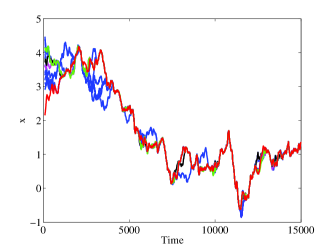
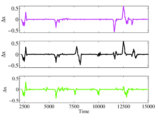
Figure 1: (Color online). a Set of trajectories of a model of colloidal particles in suspension, Eqs. (10). Different trajectories separate and recombine. b Intermittent separation of pairs of trajectories $\Delta x(t)$. The parameters are $\gamma=0.05$, $\ell_{\text{c}}=0.08$, $A=0.02$, $D=10^{-8}$.

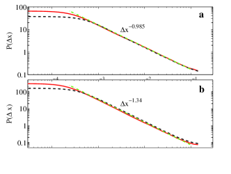
Figure 2: (Color online). The probability distribution $P_{\Delta x}$ for the model (10), for two values of $D$ ($D=3\times 10^{-10}$, full curve, and $D=10^{-9}$, dashed curves, showing fits by a power law $|\Delta x|^{-(\alpha+1)}$. The parameters are a $\gamma=0.3125$, $\ell_{\text{c}}=0.08$, $A=0.02$ b $\gamma=0.375$, $\ell_{\text{c}}=0.08$, $A=0.02$.

Beyond the point at which the underlying system becomes unstable, the system has a strange attractor, where phase points cluster on a fractal measure Ott02 . As $\lambda$ approaches zero from below, the exponent $\alpha$ in Eq. (2) approaches zero from above. When $\lambda>0$, the two-point correlation function of the strange attractor, $g(\Delta x)$, has a power-law dependence:

$$g(\Delta x)\sim|\Delta x|^{D_{2}-1},$$ (3)

where $D_{2}$ is the correlation dimension Gra+84 . Equations (2) and (3) have the same structure with the exponents related by

$$\alpha=-D_{2}$$ (4)

so that normalisable distributions of fluctuations correspond to negative values of $D_{2}$. Equation (2) therefore gives a physical meaning to a negative fractal dimension, but we should emphasise the difference between the interpretation of the two exponents. Equation (3) describes the pair correlation function for a system with no added noise, whereas Eq. (2) describes the tail of the PDF for separations when a small noise signal is added. The formal relation between our exponent $\alpha$ and the correlation dimension $D_{2}$ allows us to use recent advances in computing the correlation dimension Wil+10 ; Gus+11 ; Wil+12 to quantify our exponent $\alpha$. An alternative definition of negative fractal dimension has been offered in Man90 .

We now explain the power-law tails by introducing a cascade amplification mechanism. Consider the linearisation of Eq. (1) to give the separation between two nearby trajectories:

$$\delta\dot{x}=Z(t)\delta x+2\sqrt{D}\eta(t),$$ (5)

where

$$Z(t)=\frac{\partial v}{\partial x}(x(t),t).$$ (6)

Note that when $D=0$, $Z(t)$ is the logarithmic derivative of the separation $\delta x(t)$, and that its expectation value is the Lyapunov exponent:

$$Z(t)=\frac{\delta\dot{x}}{\delta x},\qquad\lambda=\lim_{t\to\infty}\frac{1}{t}\int_{0}^{t}{\rm d}t^{\prime}\ Z(t^{\prime})=\langle Z(t)\rangle\ .$$ (7)

We can think of $Z(t)$ as being an instantaneous Lyapunov exponent. In the case of autonomous systems with an attractor, the attractor must be a fixed point in phase space, and $Z(t)$ approaches a constant $\lambda<0$ as $t\to\infty$. In this case the fluctuations are described by an OU process and the distribution $P_{\Delta x}$ is Gaussian. In cases where the dynamical system is non-autonomous, $Z(t)$ need not approach a constant value. If the external driving is a stationary stochastic process, $Z(t)$ is a fluctuating quantity with stationary statistics. The origin of the power-law tails described by (2) is that the fluctuations are amplified during periods when $Z(t)>0$. This noise amplification is independent of the initial amplitude, because the fluctuating quantity $Z(t)$ acts multiplicatively in Eq. (5). This leads to a stochastic cascade amplification process, whereby large amplitude fluctuations are built up by a succession of periods where $Z(t)>0$. The power-law tail in the fluctuation distribution arises whenever $Z(t)$ is positive for some intervals of time, however short.

In order to quantify this picture, let us consider the dynamics of the fluctuations in a logarithmic variable

$$Y={\rm ln}(\Delta x)\ .$$ (8)

Consider the tail of $P_{\Delta x}$, where the fluctuations are much larger than the driving noise, so that the term $\sqrt{2D}\eta(t)$ in (5) can be neglected. In this limit the equation of motion for $Y(t)$ is simply $\dot{Y}=Z(t)$. Because the fluctuations of $Z(t)$ are independent of $Y$, the PDF of $Y$ is expected to approach a limit which has translational invariance, up to a normalisation factor. This implies that:

$$P_{Y}\sim\exp(-\alpha Y)$$ (9)

where the constant $\alpha$ depends on the statistics of $Z(t)$ Wil+12 . The corresponding PDF of $\Delta x$ [Eq. (2)] is then obtained by writing the change of variable ${\rm d}P=P_{Y}{\rm d}Y=P_{\Delta x}{\rm d}\Delta x$. Note that when $Y\to-\infty$, or alternatively, $\Delta x\to 0$, the noise term dominates in Eq. (5), so Eq. (2) does not apply. This prevents any difficulty with the divergence of $P_{Y}$. In fact, the role of the noise term reduces to providing a natural cutoff at small separations ($\Delta x\to 0$), thus preventing potential normalisation problems. It also follows that the exponent $\alpha$ is independent of $D$, provided that $D>0$.

Next we describe a concrete and physically important example of a system that produces fluctuations described by (2). This is provided by colloidal particles in a turbulent fluid flow, with velocity field $\mbox{\boldmath$u$}(\mbox{\boldmath$x$}(t),t)$. The motion of small particles suspended in the flow is determined by viscous drag, which makes their velocity $\mbox{\boldmath$v$}(t)$ relax to that of the surrounding fluid. When the particles have a density which is much higher than that of the fluid in which they are dispersed, the viscous drag is proportional to the difference between the particle velocity and the fluid velocity at its current location (limitations of the model are discussed in Gat83 ; Max+83 ). The problem studied in this paper is based upon a one-dimensional version of this model, which includes Brownian motion of the particles:

$$\dot{x} = v+\sqrt{2D}\eta(t),$$ (10a)

$$\dot{v} = \gamma[u(x,t)-v],$$ (10b)

where $\gamma$ is proportional to the viscosity of the fluid. We consider a random velocity field with a vanishingly small correlation time, with statistics given by

$$\langle u(x,t)\rangle = 0,$$ (11a)

$$\langle u(x,t)u(x^{\prime},t^{\prime})\rangle = A^{2}\exp\left[-\frac{(x-x^{\prime})^{2}}{\ell_{\text{c}}^{2}}\right]\delta(t-t^{\prime}).\qquad$$ (11b)

All of the explicit work shown in this paper is based on Eqs. (10) and (11). This model has two very different random elements. The random velocity field $u(x,t)$ is the same for all trajectories, whereas the Brownian noise $\eta(t)$ has a different realisation for each particle trajectory. This model has been extensively analysed for $D=0$. The Lyapunov exponent, obtained in Wil+03 , was found to be negative for sufficiently large values of $\gamma$, with the attractor not being a fixed point, but a random walk. The separation of trajectories was analysed by Der+07 and the correlation dimension was investigated in Gus+11 for the case where $D_{2}\geq 0$. When $D\neq 0$, we find that the deviations of the trajectories are found to exhibit a power-law tail in their PDF, described by Eq. (2), see Fig. 2.

Consider the linearisation of Eqs. (10):

$$\delta\dot{x} = \delta v+2\sqrt{D}\eta(t),$$

$$\delta\dot{v} = \gamma\left[S(t)\delta x-\delta v\right],$$ (12)

where $S(t)=\frac{\partial u}{\partial x}(x(t),t)$ is the velocity gradient at the position of a particle, which can be modelled by a white noise signal with diffusion coefficient ${\cal D}$:

$$S(t)=\sqrt{2{\cal D}}\zeta(t)\ ,\ \ \ \ {\cal D}=\frac{A^{2}}{\ell_{\text{c}}^{2}}$$ (13)

where $\zeta(t)$ is independent of $\eta(t)$ but has the same statistical properties.

When $D=0$, from Eqs. (Stochastic Cascade Amplification of Fluctuations) and (13) we obtain the following equation of motion for $Z(t)$ (previously obtained in Wil+03 ):

$$\dot{Z}=-\gamma Z-Z^{2}+\sqrt{2{\cal D}}\zeta(t).$$ (14)

We wish to determine the PDF for $Y$ in the form (9). From Eq. (14) we can construct a Fokker-Planck equation for the joint probability density $\rho(Y,Z)$ of $Y$ and $Z$, and seek a solution in the form $\rho(Y,Z)=\exp(-\alpha Y)\rho_{Z}(Z)$ for consistency with (9). Following an approach described in Wil+10 , this leads to a differential equation for $\alpha$ in the form

$$\hat{F}\rho_{Z}(Z)+\alpha Z\rho_{Z}(Z)=0$$ (15)

where $\hat{F}$ is a differential operator defined by writing

$$\hat{F}\rho(Z)=\frac{\partial}{\partial Z}\left[(\gamma Z+Z^{2})+{\cal D}\frac{\partial}{\partial Z}\right]\rho(Z)\ .$$ (16)

Because $\partial/\partial Z$ is a left-factor of $\hat{F}$, any normalisable solution of (15) with $\alpha\neq 0$ must satisfy:

$$\int_{-\infty}^{\infty}{\rm d}Z\ Z\,\rho_{Z}(Z)=0\ .$$ (17)

Equation (17) must be imposed on any approximate solutions of (15) constructed by perturbation theory. We remark that the integral in (17) is distinct from the Lyapunov exponent, because $\rho_{Z}(Z)$ is a distribution of $Z$ which is conditional upon the value of $Y$.

In order to facilitate the analysis of (15), we replace $Z$ by a scaled variable $x$, and introduce a dimensionless parameter $\varepsilon$:

$$x(t)=\sqrt{\frac{\gamma}{{\cal D}}}Z(t)\ ,\ \ \ \ \varepsilon=\sqrt{\frac{{\cal D}}{\gamma^{3}}}\ .$$ (18)

With these definitions, Eq. (16) is replaced by

$$\frac{\partial}{\partial x}\left[x+\varepsilon x^{2}+\frac{\partial}{\partial x}\right]\rho(x)+\alpha\varepsilon x\rho(x)=0\ .$$ (19)

Our numerical results indicate that the exponent $\alpha$, determined by directly computing $P_{\Delta x}$, is a function of the scaling variable $\varepsilon$, as illustrated in Fig. 3.

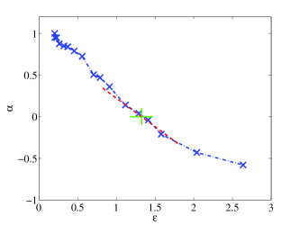
Figure 3: (Color online) Exponent $\alpha$ defined by (2) as a function of the dimensionless parameter $\varepsilon$ defined by (18). Note that $\alpha\to 1$ as $\varepsilon\to 0$ and that in the vicinity of the critical point $\varepsilon_{\rm c}$ where $\lambda=0$, we have $\alpha\sim K(\varepsilon_{\rm c}-\varepsilon)$. The dashed line uses our theoretical value for the coefficient $K$ and the cross shows the critical point location.

We consider two different perturbative approaches to determining $\alpha$ as a function of $\varepsilon$. The first is to make an expansion about $\varepsilon=0$. This can be done by following the method discussed in Wil+10 . The series expansion of $\alpha$ has only one non-zero term: $\alpha=1$, and all of the coefficients of higher powers of $\varepsilon$ are identically zero Meh . The implication is that $\alpha$ has a non-analytic dependence upon $\varepsilon$.

An alternative approach is to make a perturbative expansion about the critical point where the Lyapunov exponent changes sign. For the model underlying (10), this occurs at $\varepsilon_{\rm c}\approx 1.33\ldots$. We follow an approach used in Gus+11 (see also Sch+02 ). To leading order in $\varepsilon-\varepsilon_{\rm c}$ we obtain

$$\alpha=K(\varepsilon_{\rm c}-\varepsilon)\ .$$ (20)

Using the approach described in Gus+11 and Sch+02 the coefficient $K$ is expressed in terms of finite-dimensional integrals, whose numerical evaluation leads to $K\approx 0.688$. This value is found to be in good agreement with the results shown in Fig. 3.

We have shown that intermittency in our model leads to power-law behaviour of $P_{\Delta x}$. We now investigate the temporal variation of the signal $\Delta x(t)$. The intermittency of $\Delta x(t)$ shown in Fig. 1 can be characterised by considering the distribution of waiting time intervals $T$ over which $\Delta x(t)$ remains below a defined threshold, say $c_{\text{th}}$. Figure 4 shows the PDF $P_{T}$ of the waiting times $T$ for three different cases of noise intensity, namely $D=10^{-7}$, $10^{-8}$, and $10^{-9}$, and for the case where $\varepsilon\approx 1.118$. We observe that $P_{T}$ follows a power-law behaviour with an exponential decay at long times which can be fit to the function $P_{T}=NT^{-\tau}\exp{(-bT)}$ with an exponent $\tau=1.12\pm 0.07$, independent of $D$. Note that varying $D$ only affects the cut-off value of the exponential tail, i.e. the value of the parameter $b$: increasing $D$ decreases the range of values of $T$ over which $P_{T}$ has a power-law dependence. The inset of Fig. 4 shows that the choice of the threshold $c_{\text{th}}$ does not affect the exponent of the power-law regime, but only modifies $b$. It is important to remark that none of the mechanisms explaining the power-law distribution of inter-burst times observed in other physical systems (see e.g. Vaz+06 ; Lau+09 ; Pra+11 ) is applicable in the present problem.

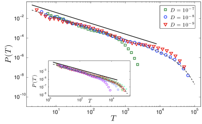
Figure 4: (Color online) PDF of the waiting times $T$ for different values of the noise intensity $D$. The dashed line corresponds to a data fit to the function $P_{T}=NT^{-\tau}\exp{(-bT)}$ with $\tau=1.12\pm 0.07$, and the solid line corresponds to a power law with exponent $-1.12$. The inlet shows results obtained by choosing different values of the threshold $c_{\text{th}}$ ($0.002\leq c_{\text{th}}\leq 0.02$) for the case of $D=10^{-8}$. The parameters of the simulation are $\gamma=0.05$, $A=0.02$ and $\ell_{\text{c}}=0.08$.

To conclude, we have explained and characterised a class of intermittent fluctuations in dynamical systems. They differ from the usual types of intermittency considered in low-dimensional systems, in that they arise when the equations of motion have additive noise, but the underlying dynamical system is stable (i.e. has a negative Lyapunov exponent). We have shown using symmetry arguments, and the assumption that the instantaneous Lyapunov exponent has positive fluctuations, that the intermittency is characterised by a power-law distribution of the magnitude of the fluctuations, and we have discussed perturbative methods for estimating the exponent $\alpha$. We have also presented evidence that there are power law distributions of other quantities, such as the inter-burst times, which is a feature common to many different intermittent systems. The stochastic cascade amplification mechanism for producing these fluctuations is generic, so that they should be observable in a wide class of systems.

References

- (1) O. Reynolds, Proc. R. Soc. Lond., 35, 84-99 (1883).
- (2) B. I. Shraiman and E. D. Siggia, Nature, 405, 639-46, (2000).
- (3) E. R. Priest and T. G. Forbes, Atron. Astroph. Rev., 10, 313-77 (2002).
- (4) P. Frantsuzov, M. Kuna, B. Janko and R. A. Marcus, Nature Physics, 4, 519-22 (2008).
- (5) R. Krahe and F. Gabbani, Nature reviews: Neuroscience, 5, 13-23 (2004).
- (6) Y. Pomeau and P. Manneville, Commun. Math. Phys., 74, 189-97, (1980).
- (7) E. Ott and J. C. Sommerer, Physics Letters A, 188, 39-47, (1994).
- (8) S. C. Venkataramani, T. M. Antonsen Jr., E. Ott and J. C. Sommerer, Physica D, 96, 66-99, (1996).
- (9) E. Ott, Chaos in Dynamical Systems, 2nd edition, University Press, Cambridbe, (2002).
- (10) Y. Pomeau, Physica D 23, 3-11 (1986).
- (11) H. Chaté and P. Manneville, Physica D 32, 409-422 (1988).
- (12) B. Eckhardt, T. M. Schneider, B. Hof and J. Westerweel, Annu. Rev. Fluid Mech. 39, 447-68 (2007).
- (13) M. Pradas, D. Tseluiko, S. Kalliadasis, D. T. Papageorgiou and G. A. Pavliotis, Phys. Rev. Lett., 106, 060602, (2011).
- (14) M. Pradas, S. Kalliadasis, D. T. Papageorgiou, G. A. Pavliotis, and D. Tseluiko. Eur. J. Appl. Math., 23, 563, (2012).
- (15) M. Wilkinson and B. Mehlig, Phys. Rev. E 68, 040101(R), (2003).
- (16) G. E. Uhlenbeck and L. S. Ornstein, Phys. Rev., 36, 823-41, (1930).
- (17) P. Grassberger and I. Procaccia, Physica D, 13, 34-54, (1984).
- (18) M. Wilkinson, K. Gustavsson and B. Mehlig, Europhys. Lett. 89, 5002 (2010).
- (19) K. Gustavsson and B. Mehlig, Phys. Rev. E 84, 045304 (2011).
- (20) M. Wilkinson, B. Mehlig, K. Gustavsson and E. Werner, Eur. Phys. J. B, 85, 18, (2012).
- (21) B. B. Mandelbrot, Physica A, 163, 306-15, (1990).
- (22) R. Gatignol, J. Méc. Théor. Appl., 1, 143?60, (1983).
- (23) M. R. Maxey and J. J. Riley, Phys. Fluids, 26, 883-9, (1983).
- (24) S. A. Derevyanko, G. Falkovich, K. Turitsyn and S. TuritsynS, J. Turbulence, 8, 1-18, (2007).
- (25) B. Mehlig and K. Gustavsson (unpublished) noted that the expansion in of the correlation dimension for (10) with is trivial.
- (26) H. Schomerus and M. Titov, Phys. Rev. E, 66, 066207, (2002).
- (27) A. Vázquez, J. G. Oliveira, Z. Dezsö, K-I. Goh, I. Kondor and A-L. Barabási, Phys. Rev. E, 73, 036127, (2006).
- (28) L. Laurson, X. Illa and M. J. Alava, J. Stat. Mech., P01019, (2009).