Finding One Community in a Sparse Graph

Abstract

We consider a random sparse graph with bounded average degree, in which a subset of vertices has higher connectivity than the background. In particular, the average degree inside this subset of vertices is larger than outside (but still bounded). Given a realization of such graph, we aim at identifying the hidden subset of vertices. This can be regarded as a model for the problem of finding a tightly knitted community in a social network, or a cluster in a relational dataset.

In this paper we present two sets of contributions: $(i)$ We use the cavity method from spin glass theory to derive an exact phase diagram for the reconstruction problem. In particular, as the difference in edge probability increases, the problem undergoes two phase transitions, a static phase transition and a dynamic one. $(ii)$ We establish rigorous bounds on the dynamic phase transition and prove that, above a certain threshold, a local algorithm (belief propagation) correctly identify most of the hidden set. Below the same threshold no local algorithm can achieve this goal. However, in this regime the subset can be identified by exhaustive search.

For small hidden sets and large average degree, the phase transition for local algorithms takes an intriguingly simple form. Local algorithms succeed with high probability for $\deg_{\rm in}-\deg_{\rm out}>\sqrt{\deg_{\rm out}/e}$ and fail for $\deg_{\rm in}-\deg_{\rm out}<\sqrt{\deg_{\rm out}/e}$ (with $\deg_{\rm in}$, $\deg_{\rm out}$ the average degrees inside and outside the community). We argue that spectral algorithms are also ineffective in the latter regime. It is an open problem whether any polynomial time algorithms might succeed for $\deg_{\rm in}-\deg_{\rm out}<\sqrt{\deg_{\rm out}/e}$.

1 Introduction

1.1 Motivation

The problem of finding a highly connected subset of vertices in a large graph arises in a number of applications across science and engineering. Within social network analysis, a highly connected subset of nodes is interpreted as a community [For10]. Many approaches to data clustering and dimensionality reduction construct a ‘similarity graph’ over the data points. A highly connected subgraph corresponds to a cluster of similar data points [VL07].

A closely related problem arises in the analysis of matrix data, e.g. in microarray data analysis. In this context, researchers are often interested in a submatrix whose entries have an average value larger (or lower) than the rest [SWPN09]. Such an anomalous submatrix is interpreted as evidence of association between gene expression levels and phenotypes (e.g. medical conditions). If we consider the graph adjacency matrix, a highly connected subset of vertices corresponds indeed to a principal submatrix with average value larger than the background.

The special case of finding a completely connected subset of vertices (a clique) in a graph has been intensely studied within theoretical computer science. Assuming P$\neq$NP, the largest clique in a graph cannot be found in polynomial time. Even a very rough approximation to its size is hard to find [Has96, Kho01]. In particular, it is hard to detect the presence of a clique of size $N^{1-\varepsilon}$ in a graph with $N$ vertices.

Such hardness results motivated the study of random instances. In particular, the so-called ‘planted clique’ or ‘hidden clique problem’ [Jer92] requires to find a clique of size $k$ that is added (planted) in a random graph with edge density $1/2$. More precisely, for a subset of vertices $S\subseteq[N]$, all edges $(i,j)$, with $\{i,j\}\subseteq S$ are present. All other edges are present independently with probability $1/2$. Such a clique can be found reliably by exhaustive search as soon as $k\geq 2(1+\varepsilon)\log_{2}N$ [GM75]. However, despite many efforts, no algorithm is known that achieves this goal for $k\ll\sqrt{N}$ [AKS98, FK00, DGGP14]. In other words, the problem of finding cliques of size $2\log_{2}N\ll k\ll\sqrt{N}$ is solvable, but possibly hard. Proving that indeed it is computationally hard to find cliques in this regime is an outstanding problem in theoretical computer science.

For general polynomial algorithms, it is known since [AKS98] that a clique of size $\delta\sqrt{N}$ can be found in time $N^{O(\log(1/\delta))}$ for any $\delta>0$ fixed. Hence, if we allow any time complexity polynomial in $N$, then the question is whether the planted clique can be found for $k=o(\sqrt{N})$.

A more stringent computational constraint requires that the clique is found in nearly-linear time, i.e. in time of order $O(N^{2}(\log N)^{c})$. Note that the number of bits required to encode an instance of the problem is of order $N^{2}$, so $N^{2}(\log N)^{c}$ is a logarithmic multiple of the time required to read an instance. Dekel, Gurel-Gurevittch and Peres [DGGP14] developed a linear-time algorithm (i.e. with complexity $O(N^{2})$) that finds the hidden clique with high probability, provided $k>1.261\sqrt{N}$. In [DM14b] it was proved that, if $k>(1+\varepsilon)\sqrt{N/e}$, then there exists a message passing algorithm that finds with high probability the clique with $O(N^{2}\log N)$ operations. The same paper provided evidence that a certain class of ‘local’ algorithms fails at the same threshold. Among other motivations, the present paper generalizes and supports the existence of a fundamental threshold for local algorithms –at least in the sparse graph setting.

1.2 Rigorous contributions

In the present paper, we consider the problem of finding a highly connected subset of vertices in a sparse graph, i.e. in a graph with bounded average degree. In this case, the hidden set size must scale linearly with $N$ to obtain a non-trivial behavior. Somewhat surprisingly, we find that the phase transition ‘at $1/\sqrt{e}$’ leaves a trace also in the sparse regime.

More precisely, we consider a random graph generated as follows. We select a subset of vertices $S$ of size $\kappa N$, uniformly at random given its size. We connect any two vertices in the set independently with probability $a/N$. Any other edge is added independently with probability $b/N$, $b<a$. The problem distribution is therefore parametrized by $a,b,\kappa\in\mathbb{R}$ and we will be therefore interested in the limit $N\to\infty$, with $a,b,\kappa$ fixed. A more intuitive parametrization is obtained by replacing $a,b$ with the average degrees for vertices $i\in S$, and $i\not\in S$ denoted, respectively, by $\deg_{\rm in}$, $\deg_{\rm out}$

Our main rigorous result is a sharp phase transition in the following double asymptotics:

• First $N\to\infty$. This corresponds to considering large graphs.

• Then $\kappa\to 0$ and $\deg_{\rm in},\deg_{\rm out}\to\infty$. This corresponds to focusing on small hidden sets, but still linear in $N$. The requirement $\deg_{\rm in},\deg_{\rm out}\to\infty$ is a necessary consequence of $\kappa\to 0$: it can be shown that otherwise the hidden set cannot possibly be detected.

Our main rigorous result (Theorem 1) establishes that, in the above double asymptotics, a phase transition takes place for local algorithms at

$$\deg_{\rm in}-\deg_{\rm out}=\sqrt{\frac{\deg_{\rm out}}{e}}\,.$$ (1)

Namely, we consider the problem of testing whether a vertex $i$ is in $S$ or not. We say that such a test is reliable if, in the above limit, the fraction of incorrectly estimated vertices vanishes in expectation. Then:

• For $\deg_{\rm in}-\deg_{\rm out}>(1+\varepsilon)\sqrt{\deg_{\rm out}/e}$, a local algorithm can estimate reliably $S$ in time of the order of the number of edges. This is achieved for instance, by the belief propagation algorithm.

• For $\deg_{\rm in}-\deg_{\rm out}<(1-\varepsilon)\sqrt{\deg_{\rm out}/e}$, no local algorithm can reliably reconstruct $S$.

Analogously to the classical hidden clique problem, there is a large gap between what can be achieved by local algorithms, and optimal estimation with unbounded computational resources. Proposition 4.1 estabilishes that exhaustive search will find $S$ in exponential time, as soon as $\deg_{\rm in}-\deg_{\rm out}>\varepsilon\sqrt{\deg_{\rm out}/e}$ for some positive $\varepsilon$ (in the same double limit).

Note that, in both cases, a small fraction of the vertices in $S$ remains undetected because of the graph sparsity, for any $\deg_{\rm in}<\infty$. In particular, the number of vertices of degree $0$ is linear in $N$, and such nodes cannot be identified.

Let us finally mention the degree of a vertex $i$ is a Poisson with mean $\deg_{\rm in}$ if $i\in S$ and mean $\deg_{\rm out}$ if $i\not\in S$. Hence, the degree standard deviation (outside $S$) is $\sqrt{\deg_{\rm out}}$. Therefore, the ratio $(\deg_{\rm in}-\deg_{\rm out})/\sqrt{\deg_{\rm out}}$ is the difference in mean degree divided by the standard deviation, and has the natural interpretation of a ‘signal-to-noise ratio.’

1.3 Non-rigorous contributions

While our rigorous analysis focuses on the limit $\kappa\to 0$ and $\deg_{\rm in},\deg_{\rm out}\to\infty$ (after $N\to\infty$), we will use the cavity method from spin glass theory to investigate the model behavior for arbitrary $\deg_{\rm in},\deg_{\rm out},\kappa$ (in the $N\to\infty$ limit) or, equivalently, arbitrary $a,b,\kappa$.

We will use two approaches to obtain concrete predictions from the cavity method:

• For general $a,b$ (bounded degree), we derive the cavity predictions for local quantities, as well as for the free energy density. We show that this indeed coincide (up to a shift) with the mutual information per variable between the hidden set $S$ and the observed graph $G$.

  We use the ‘population dynamics’ (or ‘sampled density evolution’) algorithm [MP01, RU08, MM09] to solve numerically the cavity equations.

• We then consider the limit of large $a,b$ (large degree) for arbitrary $\kappa$. In order to obtain a non-trivial limit, the signal-to-noise ratio $\lambda=\kappa^{2}(a-b)^{2}/[(1-\kappa)b]$ is kept fixed in this limit, together with $\kappa\in[0,1]$.

  The cavity equations simplify in this limit (the cavity field distributions become Gaussian), and we can derive an exact phase diagram, without recourse to intensive numerical methods, cf. Figure 5.

This two approaches are complementary in that the large-degree asymptotics yields closed-form expressions. The qualitative features of the resulting phase diagram should remain unchanged at moderately small values of $a,b$. Our population dynamics analysis confirms this.

As already mentioned, one of the motivations for the present work was to better understand the computational phase transition discovered in [DM14b] for the classical hidden clique problem. For background edge density $1/2$, this takes place when the size of the hidden clique is $k\approx\sqrt{N/e}$. This phase transition can indeed be formally recovered as a dense limit of the results presented in this paper.

More precisely, the phase transition for hidden cliques [DM14b] is captured by Eq. (1), once we rewrite the latter in terms ${\rm var}_{\rm out}$, the variance of the degrees of nodes $i\not\in S$. In the sparse regime, the degree is approximately Poisson distributed, and hence ${\rm var}_{\rm out}\approx\deg_{\rm out}$. Therefore Eq. (1) can be rewritten as $(\deg_{\rm in}-\deg_{\rm out})/\sqrt{{\rm var}_{\rm out}}=1/\sqrt{e}$ For the classical (dense) hidden clique problem, we have $\deg_{\rm out}=(N-1)/2$, $\deg_{\rm in}=(N+k-2)/2$ and ${\rm var}_{\rm out}=(N-1)/4$, and hence we recover the condition $k\approx\sqrt{N/e}$.

From a different perspective, the present work offers a statistical mechanics interpretation of the phase transitions in the hidden clique problem. Namely, the latter can be formally recovered as the $\kappa\to 0$ limit of the phase diagram in Figure 5 below. In particular, the computational phase transition at $k=\sqrt{N/e}$ corresponds to a dynamical phase transition (a spinodal point) in the underlying statistical mechanics model.

1.4 Paper outline

The rest of the paper is organized as follows. In the next section we define formally our model and some related notations. Section 3 derives the phase diagram using the cavity method. In particular, we show that the model undergoes two phase transitions as the signal-to-noise ratio increases (for $k/N$ small enough): a static phase transition and a dynamic one, The two phase transitions are well separated. Section 4 presents rigorous bounds on the behavior of local algorithms and exhaustive search, that match the above phase transitions for small $k/N$. This section is self-contained and the interested reader can move directly to it, after the model definition (some useful, but elementary results are presented in Section 3.3). Proofs are deferred to the appendix. Finally, Section 5 positions our results in the context of recent literature.

Several research communities have been working on closely related problems: statistical physics, theoretical computer science, machine learning, statistics, information theory. We tried to write a paper that could be accessible to researchers with different backgrounds, both in terms of tools and of language. We apologize for any redundancy that might have followed from this approach.

Notations

We use $[\ell]=\{1,\dots,\ell\}$ to denote the set of first $\ell$ integers, and $|A|$ to denote the size (cardinality) of set $A$.) For a set $V$, we write $(i,j)\subseteq V$ to indicate that $(i,j)$ runs over all unordered pairs of distinct elements in $V$. For instance, for a symmetric function $F(i,j)=F(j,i)$, we have

$$\prod_{(i,j)\subseteq[N]}F(i,j)\equiv\prod_{1\leq i<j\leq N}F(i,j)\,.$$ (2)

If instead $E$ is a set of edges over the vertex set $V$ (unordered pairs with elements in $V$) we write $(i,j)\in E$ to denote elements of $E$.

We use ${\sf N}(\mu,\sigma^{2})$ to denote the Gaussian distribution with mean $\mu$ and variance $\sigma^{2}$. Other classical probability distributions are denoted in a way that should be self-explanatory (Bernoulli$(p)$, Poisson$(c)$, and so on).

2 Model definition

We consider a random graph $G_{N}=(V_{N},E_{N})$ with vertex set $V_{N}=[N]\equiv\{1,\dots,N\}$ and random edges generated as follows. A set $S\subseteq V_{N}$ is chosen at random. Introducing the indicator variables

$$x_{i}=\begin{cases}1&\;\;\mbox{if $i\in S$,}\\ 0&\;\;\mbox{otherwise,}\end{cases}$$ (3)

we let $x_{i}\in\{0,1\}$ independently with

$${\mathbb{P}}\big{(}x_{i}=1\big{)}=\kappa\,.$$ (4)

In particular $|S|$ is a binomial random variable, and is tightly concentrated around its mean $\mathbb{E}|S|=\kappa N$. Edges are independent given $S$, with the following probability for $i,j\in V_{N}$ distinct:

$${\mathbb{P}}\big{\{}(i,j)\in E_{N}|S\big{\}}=\begin{cases}a/N&\;\;\mbox{if $\{i,j\}\subseteq S$,}\\ b/N&\;\;\mbox{otherwise.}\end{cases}$$ (5)

We let $x=(x_{1},\dots,x_{N})$ denote the vector identifying $S$. By using Bayes theorem, the conditional distribution of $x$ given $G$ is easily written

$$\tilde{p}_{G}(x)\equiv{\mathbb{P}}(x|G)=\frac{1}{\widetilde{Z}(G)}\prod_{i\in[N]}\Big{(}\frac{\kappa}{1-\kappa}\Big{)}^{x_{i}}\prod_{(i,j)\subseteq[N]}\Big{(}\frac{1-a/N}{1-b/N}\Big{)}^{x_{i}x_{j}}\prod_{(i,j)\in E}\rho_{N}^{x_{i}x_{j}}\,,$$ (6)

where $\rho_{N}\equiv(a/b)\big{(}(1-b/N)/(1-a/N)\big{)}$.

We next replace the last probability distribution with one that is equivalent as $N\to\infty$, and slightly more convenient for the cavity calculations of the next section. (These simplifications will not be used to prove the rigorous bounds in Section 4.) We first note that, as $N\to\infty$, we have $\rho_{N}\to\rho$ with

$$\rho\equiv\frac{a}{b}\,.$$ (7)

Next, letting $|x|\equiv\sum_{i=1}^{N}x_{i}$, we can rewrite the second product in Eq. (6) as

$$\prod_{(i,j)\subseteq[N]} \Big{(}\frac{1-a/N}{1-b/N}\Big{)}^{x_{i}x_{j}}=\Big{(}\frac{1-a/N}{1-b/N}\Big{)}^{\binom{|x|}{2}}=C\,\Big{(}\frac{1-a/N}{1-b/N}\Big{)}^{(2\kappa N-1)(|x|-\kappa N)/2}\cdot\Big{(}\frac{1-a/N}{1-b/N}\Big{)}^{\frac{1}{2}(|x|-\kappa N)^{2}}$$ (8)

with

$$C=\Big{(}\frac{1-a/N}{1-b/N}\Big{)}^{\frac{1}{2}\kappa N(\kappa N-1)}\,,$$ (9)

a constant independent of $x$. Notice that $|x|\sim{\rm Binom}(N,\kappa)$ is tightly concentrated around $\mathbb{E}\{|x|\}=\kappa N$. In particular $|x|=\kappa N+O(\sqrt{N})$ with high probability, and therefore the last term in Eq. (8) is of order $\Theta(1)$. We will neglect it, thus obtaining

$$\prod_{(i,j)\subseteq[N]} \Big{(}\frac{1-a/N}{1-b/N}\Big{)}^{x_{i}x_{j}}\approx C^{\prime}\,\Big{(}\frac{1-a/N}{1-b/N}\Big{)}^{\kappa N(|x|-\kappa N)}\approx C^{\prime\prime}\,e^{-\kappa(a-b)|x|}\,.$$ (10)

The error incurred by neglecting the last term in Eq. (8) can be corrected by considering the following approximate conditional distribution of $x$ given the graph $G$

$$p_{G}(x)=\frac{1}{Z(G)}\;\prod_{(i,j)\in E}\rho^{x_{i}x_{j}}\prod_{i\in V}\gamma^{x_{i}}\,{\mathbb{I}}\Big{(}\sum_{i\in V_{N}}x_{i}=\kappa N\Big{)}$$ (11)

where ${\mathbb{I}}(A)$ is the indicator function on condition $A$ and

$$\gamma \equiv e^{-\kappa(a-b)}\Big{(}\frac{\kappa}{1-\kappa}\Big{)}\,.$$ (12)

Note that we multiplied $\tilde{p}_{G}(\,\dot{\,})$ by the indicator function ${\mathbb{I}}\Big{(}\sum_{i\in V_{N}}x_{i}=\kappa N\Big{)}$. This can be interpreted as replacing the i.i.d. Bernoulli distribution (4) with the uniform distribution over $S$ with $|S|=\kappa N$, which is immaterial as long as local properties of $\tilde{p}_{G}(x)$ are considered.

In the following, we shall compare different reconstruction methods. Any such method corresponds to a function $T_{i}(G)\in\{0,1\}$ of vertex $i$ and graph $G$, with the interpretation

$$T_{i}(G)=\begin{cases}1&\mbox{ if $i$ is estimated to be in $S$},\\ 0&\mbox{ if $i$ is estimated not to be in $S$}.\end{cases}$$ (13)

We characterize such a test through its rescaled success probability

$${\rm P}_{\rm succ}^{(N)}(T)={\mathbb{P}}\big{(}T_{i}(G)=1\big{|}i\in S\big{)}+{\mathbb{P}}\big{(}T_{i}(G)=0\big{|}i\not\in S\big{)}-1\,.$$ (14)

Note that a trivial test (assigning $T_{i}(G)\in\{0,1\}$ at random independently of $G$) achieves ${\rm P}_{\rm succ}^{(N)}(T)=0$, while a perfect test has ${\rm P}_{\rm succ}^{(N)}(T)=1$. We shall often omit the arguments $T$, $n$ from ${\rm P}_{\rm succ}^{(N)}(T)$ in the following.

We note in passing that the optimal estimator with respect to the metric (14) is the maximum-likelihood estimator

$$T_{i}^{\rm opt}(G)=\begin{cases}1&\mbox{ if ${\mathbb{P}}(G|i\in S)\geq{\mathbb{P}}(G|i\not\in S)$,}\\ 0&\mbox{ if ${\mathbb{P}}(G|i\in S)<{\mathbb{P}}(G|i\not\in S)$.}\end{cases}$$ (15)

Namely, for any other estimator $T$, we have ${\rm P}_{\rm succ}^{(N)}(T)\leq{\rm P}_{\rm succ}^{(N)}(T^{\rm opt})$ (see, for instance, the textbook [LC98] for a proof of this fact). The resulting success probability coincides with the total variation distance between the conditional distribution of $G$ given the two hypotheses $i\in S$ and $i\not\in S$. Recall that, given two probability measures $p,q$ on the same finite space $\Omega$, their total variation distance is defined as $\|p(\,\cdot\,)-q(\,\cdot\,)\|_{\mbox{\rm\tiny TV}}\equiv(1/2)\sum_{\omega\in\Omega}|p(\omega)-q(\omega)|$. Then we have

$${\rm P}_{\rm succ}^{(N)}(T)\leq{\rm P}_{\rm succ}^{(N)}(T^{\rm opt})=\|{\mathbb{P}}(G\in\cdot|i\in S)\geq{\mathbb{P}}(G\in\cdot|i\not\in S)\|_{\mbox{\rm\tiny TV}}\,.$$ (16)

3 Phase transitions via cavity method

In this section we use the cavity method to derive an exact phase diagram of the model. It is convenient to introduce the following signal-to-noise-ratio parameter:

$$\lambda\equiv\frac{(\deg_{\rm out}-\deg_{\rm in})^{2}}{(1-\kappa)\deg_{\rm out}}\,.$$ (17)

Using the fact that the degree outside $S$ is Poisson with mean $\deg_{\rm out}=b$, and inside is Poisson with mean $\deg_{\rm in}=\kappa a+(1-\kappa)b$, we also have

$$\lambda=\frac{\kappa^{2}(a-b)^{2}}{(1-\kappa)b}\,.$$ (18)

We will therefore think in terms of the three independent parameters: $\kappa$ (the relative size of $|S|$); $b$ (the average degree in the background); $\lambda$ (the signal-to-noise ratio).

We generically find two solutions of the cavity recursion, that possibly coincide depending on the parameters values. This correspond to two distinct phases of the statistical mechanics models, and also have a useful algorithmic interpretation, which will be spelled out in detail in Section 3.3.

Initializing the recursion with the ‘exact solution’ of the reconstruction problem (‘plus’ initialization), we converges to a ferromagnetic fixed point. This provides an upper bound on the performance of any reconstruction algorithm. Initializing the recursion with a completely oblivious initialization (‘free’ initialization), we converge to a paramagnetic fixed point. This also corresponds to the performance of the best possible local algorithm (see next section for a formal definition). A very similar qualitative picture is found in other inference problems on random graphs, one early example being the analysis of sparse graph codes [RU08, MM09]. An important simplification is that we do not expect replica-symmetry breaking in these models [Nis01, Mon08].

Depending on the model parameters, we encounter two types of behaviors as $\lambda$ increases.

• For large $\kappa$ or small $b$, the two fixed points mentioned above coincide for all $\lambda$ and no phase transition takes place.

• For small $\kappa$ and large $b$, two phase transitions take place: a static phase transition at $\lambda_{\rm s}(\kappa,b)$ and a dynamic phase transition at a larger value $\lambda_{\rm d}(\kappa,b)$. In addition, a spinodal point occurs at $\lambda_{\rm sp}(\kappa,b)<\lambda_{\rm s}(\kappa,b)<\lambda_{\rm d}(\kappa,b)$.

  For $\lambda<\lambda_{\rm sp}$ the two fixed point above coincide, and yield bad reconstruction. For $\lambda>\lambda_{\rm d}$ they coincide and yield good reconstruction. In the intermediate phase $\lambda_{\rm sp}\leq\lambda\leq\lambda_{\rm d}$, the two fixed points do not coincide. The relevant fixed point for Bayes-optimal reconstruction corresponds to the one of smaller free energy, and the transition between the two takes place at $\lambda_{\rm s}$.

The reader might consult Fig. 5 for an illustration. Also, a very similar phase diagram was obtained in the related problem of sparse principal component analysis in [DM14a, LKZ15].

3.1 Cavity equations and population dynamics

Fixing $i$, let ${\mathbb{P}}(\,\cdot\,|i\in S)$ (respectively ${\mathbb{P}}(\,\cdot\,|i\not\in S)$) be the law of $G$ subject to $S$ containing (respectively –not containing) vertex $i$. Consider the random variable

$$\xi_{i}(G)\equiv\log\frac{{\mathbb{P}}(x_{i}=1|G)}{{\mathbb{P}}(x_{i}=0|G)}\,.$$ (19)

The likelihood ratio test (maximizing ${\rm P}_{\rm succ}$) amounts to choosing

$$T^{\rm opt}_{i}(G)={\mathbb{I}}\Big{(}\xi_{i}(G)\geq\log\frac{\kappa}{1-\kappa}\Big{)}\,.$$ (20)

As $N\to\infty$, the distribution of $\xi_{i}(G)$ under ${\mathbb{P}}(\,\cdot\,|i\in S)$ converges to the law of a certain random variable $\xi_{1}$, and the distribution of $\xi_{i}(G)$ under ${\mathbb{P}}(\,\cdot\,|i\not\in S)$ converges instead to $\xi_{0}$. The cavity method allows to write fixed point equations for these limit distributions. We omit details of the derivation since they are straightforward given the model (11), and since it is sufficient here to consider the replica-symmetric version of the method. General derivations can be found in [MM09, Chapter 14]. A closely related calculation is carried out in [DKMZ11a], which studies a more general random graph model, the so-called stochastic block model.

The distribution of $\xi_{1}$, $\xi_{0}$ are fixed point of the following recursion (the symbol $\stackrel{{\scriptstyle{\rm d}}}{{=}}$ means that the distributions of quantities on the two sides are equal)

$$\xi_{0}^{(t+1)} \stackrel{{\scriptstyle{\rm d}}}{{=}}h+\sum_{i=1}^{L_{00}}f(\xi^{(t)}_{0,i})+\sum_{i=1}^{L_{01}}f(\xi^{(t)}_{1,i})\,,$$ (21)

$$\xi_{1}^{(t+1)} \stackrel{{\scriptstyle{\rm d}}}{{=}}h+\sum_{i=1}^{L_{10}}f(\xi^{(t)}_{0,i})+\sum_{i=1}^{L_{11}}f(\xi^{(t)}_{1,i})\,.\$$ (22)

Here $\xi^{(t)}_{0/1,i}$ are independent copies of $\xi^{(t)}_{0/1}$. Further $L_{00}\sim{\rm Poisson}((1-\kappa)b)$, $L_{01}\sim{\rm Poisson}(\kappa b)$, $L_{10}\sim{\rm Poisson}((1-\kappa)b)$, $L_{11}\sim{\rm Poisson}(\kappa a)$, are independent Poisson random variables, independent of the $\{\xi^{(t)}_{0,i}\}$. Finally,

$$h=\log\gamma=-\kappa(a-b)-\log\Big{(}\frac{1-\kappa}{\kappa}\Big{)}\,,$$ (23)

and the function $f:\mathbb{R}\to\mathbb{R}$ is given by

$$f(\xi)\equiv\log\Big{(}\frac{1+\rho\,e^{\xi}}{1+e^{\xi}}\Big{)}\,.$$ (24)

(Recall that $\rho=a/b$, cf. Eq. (7).)

The cavity method predicts that the asymptotic distribution of $\xi_{i}(G)$ (conditional to $i\in S$ or $i\not\in S$) is a fixed point of Eqs. (21), (22). In order to find the fixed points, we iterate these distributional equations with two types of initial conditions (that correspond, respectively, to the poor reconstruction and good reconstruction phases)

$${\rm free}\;\;: \;\;\;\begin{cases}\xi^{(0),\mbox{\rm\tiny fr}}_{0}=\log(\kappa/(1-\kappa))\,,\\ \xi^{(0),\mbox{\rm\tiny fr}}_{1}=\log(\kappa/(1-\kappa))\,,\end{cases}$$ (25)

$${\rm plus}\;\;: \;\;\;\begin{cases}\xi^{(0),\mbox{\rm\tiny pl}}_{0}=-\infty\,,\\ \xi^{(0),\mbox{\rm\tiny pl}}_{1}=+\infty\,.\end{cases}$$ (26)

We refer to Section 3.3 for the interpretation and monotonicity properties of these conditions: in particular it can be proved that $\xi^{(t)}_{0/1}$ converge in distribution if initialized in this manner. We implemented Eqs. (21), (22) numerically using the ‘population dynamics’ method of [MP01] (also known as ‘sampled density evolution’ [RU08, MM09]).

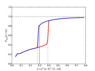
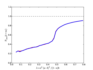
Figure 1: The success probability in the two different phases, for $\kappa=0.005$ (left), $0.020$ (right) and $b=100$ (corresponding to average degree outside the set $S$, $\deg_{\rm out}=100$). Red curves correspond ${\rm P}_{\rm succ}(\mbox{\rm fr})$ (i.e. free boundary/initial conditions), and provide to the optimal performance of local algorithms. Blue curves yield ${\rm P}_{\rm succ}(\mbox{\rm pl})$ (i.e. plus boundary/initial conditions) and yield an upper bound on the performance of any algorithm. The continuous black line at $\lambda_{\rm s}\approx 0.3$ coincides with the phase transition of Bayes-optimal estimation. These curves were computed by averaging over $10$ runs of the population dynamics algorithm with $M=10^{4}$ samples and $300$ iterations.

In Figure 1, we plot the predicted behavior of ${\rm P}_{\rm succ}$ for $b=100$ and two different values of the clique size: $\kappa\in\{0.005,0.020\}$. The success probability is predicted to be (for $N\to\infty$)

$${\rm P}_{\rm succ}={\mathbb{P}}(\xi^{(\infty)}_{1}\geq 0)+{\mathbb{P}}(\xi_{0}^{(\infty)}<0)-1\,.$$ (27)

We denote by ${\rm P}_{\rm succ}(\mbox{\rm fr})$ and ${\rm P}_{\rm succ}(\mbox{\rm pl})$ the predictions obtained with the two initializations above.

As anticipated two behaviors can be observed. For $\kappa$ sufficiently large, the curves ${\rm P}_{\rm succ}(\mbox{\rm fr})$ and ${\rm P}_{\rm succ}(\mbox{\rm pl})$ coincide for all $\lambda$. When this happens, this is also the success probability of the optimal likelihood ratio test $T^{\rm opt}$, and the latter can be effectively approximated using a local algorithm (e.g. belief propagation), see Section 3.3. For $\kappa$ small the two curves remain distinct in an intermediate interval of values: $\lambda\in(\lambda_{\rm sp},\lambda_{\rm d})$.

In this regime, the asymptotic behavior of the Bayes-optimal test is captured by the fixed point that yields the lowest free energy. It is convenient to define the rescaled free energy density as follows (assuming that the limit exists)

$$\psi\equiv\frac{\kappa^{2}}{2}\,\Big{(}a\log\frac{a}{b}-2a+2b\Big{)}-\log(1-\kappa)-\lim_{n\to\infty}\frac{1}{n}\mathbb{E}\log Z(G)\,.$$ (28)

The reason for this choice of the additive constants is that the resulting free energy is also equal to the asymptotic mutual information between the hidden set $S$ and the observed graph $G$

$$\psi=\lim_{n\to\infty}\frac{1}{N}\ {\rm I}(G;S)\,.$$ (29)

This quantity has therefore an immediate interpretation and several useful properties.

The replica symmetric cavity method (equivalently, Bethe-Peierls approximation) predicts

$$\psi=\min_{{\rm P}_{0},{\rm P}_{1}}\Psi({\rm P}_{0},{\rm P}_{1})\,,$$ (30)

where the supremum is over all probability distributions ${\rm P}_{0},{\rm P}_{1}$ over the real line satisfying the following symmetry property (see Section 3.3 for further clarification on this property):

$$\frac{{\rm d}{\rm P}_{1}}{{\rm d}{\rm P}_{0}}(\xi)=\frac{1-\kappa}{\kappa}\,e^{\xi}\,.$$ (31)

The functional $\Psi$ is defined as follows

$$\Psi =\Psi^{{\rm e}}-\Psi^{{\rm v}}+\Psi_{0}\,,$$ (32)

$$\Psi^{{\rm e}} =\frac{1}{2}\big{(}\kappa^{2}a+(1-\kappa^{2})b\big{)}\,\mathbb{E}\log\Big{\{}1+\frac{(\rho-1)\,e^{\xi_{x_{1},1}+\xi^{\prime}_{x_{2},2}}}{(1+e^{\xi_{x_{1},1}})(1+e^{\xi_{x_{2},2}}))}\Big{\}}\,,$$ (33)

$$\Psi^{{\rm v}} =\mathbb{E}\log\Big{\{}1-\kappa+\kappa\,e^{-\kappa(a-b)}\prod_{i=1}^{L_{0}}\Big{(}\frac{1+\rho\,e^{\xi_{0,i}}}{1+e^{\xi_{0,i}}}\Big{)}\prod_{j=1}^{L_{1}}\Big{(}\frac{1+\rho\,e^{\xi_{1,j}}}{1+e^{\xi_{1,j}}}\Big{)}\Big{\}}\,,$$ (34)

$$\Psi_{0} =\frac{\kappa^{2}}{2}\,\Big{(}a\log\frac{a}{b}-2a+2b\Big{)}\,.$$ (35)

Here expectation is taken with respect to the following independent random variables:

• $\{\xi_{0,i}\}$ that are i.i.d. random variables with distribution ${\rm P}_{0}$;

• $\{\xi_{1,i}\}$ that are i.i.d. random variables with distribution ${\rm P}_{1}$;

• $(x_{1},x_{2})\in\{0,1\}^{2}$ with joint distribution $p_{1,1}=\kappa^{2}a/z$, $p_{0,1}=p_{1,0}=\kappa(1-\kappa)b/z$, $p_{1,1}=(1-\kappa)^{2}b/z$, where $z=\kappa^{2}a+(1-\kappa^{2})b$.

• $(L_{0},L_{1})$ with the following mixture distribution. With probability $\kappa$: $L_{0}\sim{\rm Poisson}((1-\kappa)b)$, $L_{1}\sim{\rm Poisson}(\kappa a)$. With probability $(1-\kappa)$: $L_{0}\sim{\rm Poisson}((1-\kappa)b)$, $L_{1}\sim{\rm Poisson}(\kappa b)$.

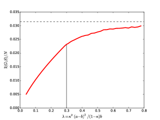
Figure 2: The free energy density (equivalently, the mutual information per vertex), for $\kappa=0.005$. The horizontal line corresponds to the maximal mutual information $H(\kappa)\approx 0.03148$., The vertical line at $\lambda_{\rm s}\approx 0.3$ corresponds to the phase transition of the Bayes-optimal estimator. This curve was computed by averaging over $10$ runs of the population dynamics algorithm with $M=10^{4}$ samples and $300$ iterations.

Let ${\rm P}_{0/1}^{\mbox{\rm\tiny pl}}$ and ${\rm P}_{0/1}^{\mbox{\rm\tiny fr}}$ the distributions of the fixed points obtained with plus and free initial conditions. In Figure 2 we plot the minimum of the corresponding Bethe free energies $\Psi(\mbox{\rm pl})=\Psi({\rm P}_{0}^{\mbox{\rm\tiny pl}},{\rm P}_{1}^{\mbox{\rm\tiny pl}})$ and $\Psi(\mbox{\rm fr})=\Psi({\rm P}_{0}^{\mbox{\rm\tiny fr}},{\rm P}_{1}^{\mbox{\rm\tiny fr}})$ for $b=100$, $\kappa=0.005$ (as obtained by the population dynamics algorithm). This is the cavity prediction for the free energy density $\psi$. The value of $\lambda$ for which $\Psi(\mbox{\rm pl})=\Psi(\mbox{\rm fr})$ corresponds to the phase transition point $\lambda_{\rm s}$ between paramagnetic and ferromagnetic phases. From the reconstruction point of view, this is the phase transition for Bayes-optimal estimation:

$$\lim_{N\to\infty}{\rm P}_{\rm succ}^{(N)}(T^{\rm opt})=\begin{cases}{\rm P}_{\rm succ}(\mbox{\rm fr})&\mbox{ for $\lambda<\lambda_{\rm s}$}\,,\\ {\rm P}_{\rm succ}(\mbox{\rm pl})&\mbox{ for $\lambda>\lambda_{\rm s}$}\,.\end{cases}$$ (36)

Notice from Figure 2 that as expected $\psi=\lim_{N\to\infty}{\rm I}(G;S)/N$ is monotone increasing in the signal-to-noise ratio $\lambda$, with $\psi\to 0$ as $\lambda\to 0$, and $\psi\to H(\kappa)$ as $\lambda\to\infty$ (here $H(\kappa)=-\kappa\log\kappa-(1-\kappa)\log(1-\kappa)$ is the entropy of a Bernoulli random variable with mean $\kappa$). Also, the curve Fig. 2 presents some ‘wiggles’ at large $\kappa$ that are due to the limited numerical accuracy of the population dynamics algorithm.

3.2 Large-degree asymptotics

In the previous section we solved numerically the distributional equations (21), (22). This approach is somewhat laborious and its accuracy is limited. Asymptotic expansions provide complementary analytical insights into the solution of these equations.

a

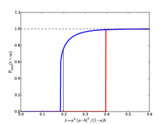
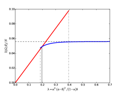
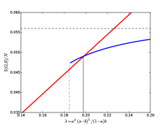
Figure 3: Limit $a,b\to\infty$ with $\lambda$ and $\kappa$ fixed. Here $\kappa=0.01$. Left frame: Success probability for free boundary condition (equivalently, local algorithms, red curve), and plus boundary condition (equivalently, general upper bound, blue curve). Center frame: free energy (equivalently, mutual information per vertex) with same boundary conditions. Right frame: zoom of the free energy curves.

Here we consider $a,b\to\infty$ with $\kappa$ fixed, and $(a-b)/b^{2}$ converging to a limit. In particular, the signal-to-noise ratio $\lambda$ is also a constant. Let us emphasize once more that these limits are taken after $N\to\infty$ and hence the graph is still sparse.

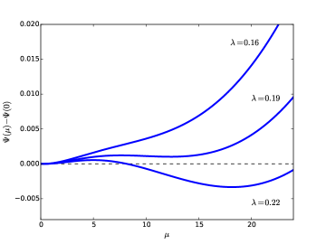
Figure 4: Limit $a,b\to\infty$ with $\lambda$ and $\kappa$ fixed. Here we plot the (shifted) free energy function $\Psi(\mu)-\Psi(0)$ for $\kappa=0.01$ and $\lambda\in\{0.16,0.19,0.22\}$. Comparing with Figure 3 we see that $0.16<\lambda_{\rm sp}(\kappa)<\lambda_{\rm s}(\kappa)$, $\lambda_{\rm sp}(\kappa)<0.19<\lambda_{\rm s}(\kappa)$, $\lambda_{\rm sp}(\kappa)<\lambda_{\rm s}(\kappa)<0.22<\lambda_{\rm d}(\kappa)$.

In this limit, the fixed points of Eqs. (21), (22) take the form

$$\xi_{0} \sim{\sf N}\Big{(}-\log\Big{(}\frac{1-\kappa}{\kappa}\Big{)}-\frac{1}{2}\,\mu,\;\mu\Big{)}\,,$$ (37)

$$\xi_{1} \sim{\sf N}\Big{(}-\log\Big{(}\frac{1-\kappa}{\kappa}\Big{)}+\frac{1}{2}\,\mu,\;\mu\Big{)}\,.$$ (38)

Further $\mu$ satisfies the fixed point equation

$$\mu=\lambda\,{\sf F}(\mu;\kappa)$$ (39)

where the function ${\sf F}(\,\cdot\,;\,\cdot\,)$ is defined by

$${\sf F}(\mu;\kappa)\equiv\mathbb{E}\Big{\{}\frac{1-\kappa}{\kappa+(1-\kappa)e^{-(\mu/2)+\sqrt{\mu}\,Z}}\Big{\}}\,,$$ (40)

with expectation being taken with respect to $Z\sim{\sf N}(0,1)$. In other words, the distributional equations (21), (22) reduced to a single nonlinear equation for the scalar $\mu$. Large $\mu$ correspond to accurate recovery.

More formally, we expect the distributional solutions of Eqs. (21), (22) to converge to solutions of Eqs. (37) to (40). We do not provide a ‘physicists’ derivation of this statement since this follows heuristically from Lemma 4.4. The latter establishes that, iterating the cavity equations Eqs. (21), (22) any fixed number of times $t$ is equivalent (in the large-degree limit) to iterating Eqs. (37) to (40).

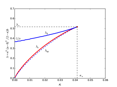
Figure 5: Phase diagram of the hidden subgraph problem in the large degree limit $a,b\to\infty$, with $\kappa=\mathbb{E}|S|/N$ (relative size of the hidden set) and $\lambda=\kappa^{2}(a-b)^{2}/((1-\kappa)b)$ (signal-to-noise ratio) fixed. The three curves are, from top to bottom $\lambda_{\rm d}(\kappa)$, $\lambda_{\rm s}(\kappa)$ and $\lambda_{\rm sp}(\kappa)$.

The free energy (32) becomes a function of $\mu$ (we still denote it by $\Psi$ with a slight abuse of notation):

$$\Psi(\mu) =\frac{1}{4}\lambda(1-\kappa)+\frac{\kappa^{2}}{4\lambda(1-\kappa)}\mu^{2}-\mathbb{E}\log\Big{\{}1-\kappa+\kappa\,\exp\Big{(}\sqrt{\mu}Z-\frac{1}{2}\mu+\mu X\Big{)}\Big{\}}\,,$$ (41)

where expectation is with respect to independent random variables $X\sim{\rm Bernoulli}(\kappa)$ and $Z\sim{\sf N}(0,1)$. Its local minima are solutions of Eq. (39).

Equation (39) can be easily solved numerically, yielding the phase diagram in Figure 5. As before, we obtain phase transitions $\lambda_{\rm sp}(\kappa)<\lambda_{\rm s}(\kappa)<\lambda_{\rm d}(\kappa)$ as long as $\kappa$ is below a critical point $\kappa<\kappa_{*}$. The critical point location is

$$\kappa_{*}\approx 0.04139\,,\;\;\;\;\;\;\;\;\;\lambda_{*}\approx 0.5176\,.$$ (42)

The free energy $\Psi(\mu)$ has two local minima $\mu^{\mbox{\rm\tiny pl}}>\mu^{\mbox{\rm\tiny fr}}$ for $\kappa<\kappa_{*}$, $\lambda\in(\lambda_{\rm sp}(\kappa),\lambda_{\rm d}(\kappa))$, and one local minimum otherwise. The local minimum $\mu^{\mbox{\rm\tiny pl}}$ is the global minimum for $\lambda>\lambda_{\rm s}(\kappa)$, while $\mu^{\mbox{\rm\tiny fr}}$ is the global minimum for $\lambda<\lambda_{\rm s}(\kappa)$. We refer to Figures 3 and 4 for illustration.

Of particular interest is the case of small hidden subsets, i.e. the limit $\kappa\to 0$ (note that $|S|$ is still linear in $N$). For small $\kappa$ we have $\lim_{\kappa\to 0}{\sf F}(\mu;\kappa)={\sf F}(\mu;0)=e^{\mu}$. Hence the solutions (39) that stay bounded converges to the solution of

$$\mu=\lambda\,e^{\mu}\,.$$ (43)

This equation has two solutions for $\lambda<1/e$ and no solution for $\lambda>1/e$. This implies that

$$\lim_{\kappa\to 0}\lambda_{\rm d}(\kappa)=\frac{1}{e}\,,$$ (44)

which is the result announced in Eq. (1). It is also easy to see that $\lambda_{\rm s}(\kappa),\lambda_{\rm sp}(\kappa)\to 0$ as $\kappa\to 0$.

3.3 Algorithmic interpretation

The distributional equations (21) and (22) define a sequence of probability distributions indexed by $t\in\{0,1,2,\dots\}$. More precisely, for every $t$ the recursion defines the probability distributions ${\rm P}_{0}^{(t)}$ (the distribution of $\xi_{0}^{(t)}$) and ${\rm P}_{1}^{(t)}$ (the distribution of $\xi_{1}^{(t)}$). When specialized to the free/plus initial conditions (cf. Eqs.  (25),  (25)), these probability distributions have a simple and useful interpretation that we will now explain.

Define ${\sf B}_{t}(G,i)$ to be the ball of radius $t$ centered at $i\in V$, in graph $G$. Namely, this is the subset of vertices of $G$ whose distance from $i$ is at most $t$. By a slight abuse of notation, this will also denote the subgraph induced in $G$ by those vertices. The following remarks are straightforward.

Free boundary condition. Consider the optimal test $T_{i}(G)$ among those that only use local information. In other words, $T_{i}(G)$ is the optimal test that is a function of ${\sf B}_{t}(G,i)$. This is again a likelihood ratio test. Concretely, we can define the log-likelihood ratio

$$\xi_{i}(G;t)\equiv\log\frac{{\mathbb{P}}(x_{i}=1|{\sf B}_{t}(G,i))}{{\mathbb{P}}(x_{i}=0|{\sf B}_{t}(G,i))}\,.$$ (45)

Then the optimal test takes the form $T_{i}(G)={\mathbb{I}}(\xi_{i}(G)\geq\log[\kappa/(1-\kappa)])$ (if we are interested in maximizing ${\rm P}_{\rm succ}^{(N)}(T)$) or $T_{i}(G)={\mathbb{I}}(\xi_{i}(G)\geq 0)$ (if we are interested in minimizing the expected number of incorrectly assigned vertices).

Fixing the depth parameter $t$, the distribution of $\xi_{i}(G;t)$ converges (as $N\to\infty$) to ${\rm P}_{0}^{(t),\mbox{\rm\tiny fr}}$ for $i\in S$, and to ${\rm P}_{1}^{(t),\mbox{\rm\tiny fr}}$ for $i\not\in S$. Mathematically, for any fixed $i$

$$\xi_{i}(G;t) \stackrel{{\scriptstyle{\rm d}}}{{\Rightarrow}}\xi_{1}^{(t),\mbox{\rm\tiny fr}}\;\;\;\;\;\;\mbox{ under }{\mathbb{P}}(\,\cdot\,|i\in S)\,,$$ (46)

$$\xi_{i}(G;t) \stackrel{{\scriptstyle{\rm d}}}{{\Rightarrow}}\xi_{0}^{(t),\mbox{\rm\tiny fr}}\;\;\;\;\;\;\mbox{ under }{\mathbb{P}}(\,\cdot\,|i\not\in S)\,.$$ (47)

In particular, for any fixed $t$, the success probability

$${\rm P}_{\rm succ}(t;\mbox{\rm fr})={\rm P}_{0}^{(t),\mbox{\rm\tiny fr}}\Big{(}\xi<\log[\kappa/(1-\kappa)]\Big{)}+{\rm P}_{1}^{(t),\mbox{\rm\tiny fr}}\Big{(}\xi\geq\log[\kappa/(1-\kappa)]\Big{)}-1\,$$ (48)

is the maximum asymptotic success probability achieved by any test that is $t$-local (in the sense of being a function of depth-$t$ neighborhoods). It follows immediately from the definition that ${\rm P}_{\rm succ}(t;\mbox{\rm fr})$ is monotone increasing in $t$. Its $t\to\infty$ limit ${\rm P}_{\rm succ}(\mbox{\rm fr})$ is the maximum success probability achieved by any local algorithm. This quantity was computed through population dynamics in the previous section, see Figure 1.

Plus boundary condition. Let $\overline{\sf B}_{t}(G,i)$ be the complement of ${\sf B}_{t}(G,i)$, i.e. the set of vertices of $G$ that have distance at least $t$ from $i$. Then $\xi^{(t),\mbox{\rm\tiny pl}}_{0/1}$ has the interpretation of being the log-likelihood ratio, when information is revealed about the labels of vertices in $\overline{\sf B}_{t-1}(G,i)$. Namely, if we define

$$\xi^{\prime}_{i}(G;t)\equiv\log\frac{{\mathbb{P}}(x_{i}=1|{\sf B}_{t}(G,i),x_{\overline{\sf B}_{t}(G,i)})}{{\mathbb{P}}(x_{i}=0|{\sf B}_{t}(G,i),x_{\overline{\sf B}_{t}(G,i)})}\,,$$ (49)

then we have

$$\xi^{\prime}_{i}(G;t) \stackrel{{\scriptstyle{\rm d}}}{{\Rightarrow}}\xi_{1}^{(t),\mbox{\rm\tiny pl}}\;\;\;\;\;\;\mbox{ under }{\mathbb{P}}(\,\cdot\,|i\in S)\,,$$ (50)

$$\xi^{\prime}_{i}(G;t) \stackrel{{\scriptstyle{\rm d}}}{{\Rightarrow}}\xi_{0}^{(t),\mbox{\rm\tiny pl}}\;\;\;\;\;\;\mbox{ under }{\mathbb{P}}(\,\cdot\,|i\not\in S)\,.$$ (51)

In particular, ${\rm P}_{\rm succ}(\mbox{\rm pl})$ is an upper bound on the performance of any estimator. In the previous section we computed this quantity numerically through population dynamics.

Let us finally comment on the relation (31) between ${\rm P}_{0}$ and ${\rm P}_{1}$. This is an elementary consequence of Bayes formula: consequences of this relation have been useful in statistical physics under the name of ‘Nishimori property’ [Nis01]. It is also known in coding theory as ‘symmetry condition’ [RU08]. Consider the general setting of two random variables $X,Y$, with $X\in\{0,1\}$, ${\mathbb{P}}(X=1)=\kappa$, and let $\xi(Y)=\log[{\mathbb{P}}(X=1|Y)/{\mathbb{P}}(X=0|Y)]$. Then for any interval $A$ (with non-zero probability), applying Bayes formula,

$${\mathbb{P}}(\xi(Y)\in A|X=1) =\frac{{\mathbb{P}}(\xi(Y)\in A;X=1)}{{\mathbb{P}}(X=1)}$$ (52)

$$=\frac{1}{\kappa}\,\mathbb{E}\big{\{}{\mathbb{I}}(\xi(Y)\in A){\mathbb{P}}(X=1|Y)\big{\}}=\frac{1}{\kappa}\,\mathbb{E}\big{\{}{\mathbb{I}}(\xi(Y)\in A)\,{\mathbb{I}}(X=0)e^{\xi(Y)}\big{\}}$$ (53)

$$=\frac{1-\kappa}{\kappa}\,\mathbb{E}\big{\{}{\mathbb{I}}(\xi(Y)\in A)\,e^{\xi(Y)}|X=0\big{\}}\,,$$ (54)

which is the claimed property.

4 Rigorous results

In the previous section we relied on the non-rigorous cavity method from spin glass theory to derive the phase diagram. Most notably we used numerical methods, and formal large-degree asymptotics to study the distributional equations (21), (22). Here we will establish rigorously some key implications of the phase diagram, namely:

• By exhaustive search over all subsets of $k$ vertices in $G$, we can estimate $S$ accurately for any $\lambda>0$ and $\kappa$ small.

• Local algorithms succeed in reconstructing accurately $S$ if $\lambda>1/e$, and fail for $\lambda<1/e$ (assuming large degrees and $\kappa$ small).

4.1 Exhaustive search

Given a set of vertices $R\subseteq[N]$, we let $E(R)$ denote the number of edges with both endpoints in $R$. Exhaustive search maximizes this quantity among all the sets that have the ‘right size.’ Namely, it outputs

$$\widehat{S}=\arg\max_{R\subseteq[N]}\Big{\{}\,E(R)\,:|R|=\lfloor\kappa n\rfloor\Big{\}}\,.$$ (55)

(If multiple maximizers exist, one of them is selected arbitrarily.) We can also define a test function $T_{i}(G)$ by letting $T^{\mbox{\rm\tiny ex}}_{i}(G)=1$ for $i\in\widehat{S}$ and $T^{\mbox{\rm\tiny ex}}_{i}(G)=0$ otherwise. Note that, for $\kappa n$ growing with $n$, this algorithm is non-polynomial and hence cannot be used in practice. It provides however a useful benchmark..

We have the following result showing that exhaustive search reconstructs $S$ accurately, for any constant $\lambda$ and $\kappa$ small. We refer to Section A for a proof.

Proposition 4.1.

Let ${\rm P}_{\rm succ}^{\mbox{\rm\tiny ex}}=\lim\sup_{N\to\infty}{\rm P}_{\rm succ}^{(N),\mbox{\rm\tiny ex}}$ be the asymptotic success probability of exhaustive search and assume $\kappa<1/2$. Then

$${\rm P}_{\rm succ}^{\mbox{\rm\tiny ex}}\geq 1-\frac{2e}{\sqrt{\kappa}}\,\exp\Big{(}-\frac{\lambda(1-\kappa)b}{16\,\kappa a}\Big{)}\,.$$ (56)

In particular, we have the following large degree asymptotics as $a,b\to\infty$ with $\lambda,\kappa$ fixed

$${\rm P}_{\rm succ}^{\mbox{\rm\tiny ex}}(b=\infty)\equiv\lim\inf_{a,b\to\infty}{\rm P}_{\rm succ}^{\mbox{\rm\tiny ex}}\geq 1-\frac{2e}{\sqrt{\kappa}}\,\exp\Big{(}-\frac{\lambda(1-\kappa)}{16\,\kappa}\Big{)}\,,$$ (57)

and ${\rm P}_{\rm succ}^{\mbox{\rm\tiny ex}}(b=\infty)\to 1$ as $\kappa\to 0$ for any $\lambda>0$ fixed.

4.2 Local algorithms

We next give a formal definition of $t$-local algorithms. Let ${\cal G}_{*}$ is the space of unlabeled rooted graphs, i.e. the space of graphs with one distinguished vertex (see –for instance– [Mon15] for more details). Formally, an estimator $T_{i}(G)$ for the hidden set problem is a function $(G,i)\mapsto T(G;i)=T_{i}(G)\in\{0,1\}$. Since the pair $(G,i)$ is indeed a graph with one distinguished vertex (and the vertices labels clearly do not matter), we can view $T$ as a function on ${\cal G}_{*}$:

$$T:{\cal G}_{*}\to\{0,1\}\,.$$ (58)

The following definition formalizes the discussion in Section 3.3 (where the definition of ${\sf B}_{t}(G,i)$ is also given). The key fact about this definition is that $t$ (the ‘locality radius’) is kept fixed, while the graph size can be arbitrarily large.

Definition 4.2.

Given a non-negative integer $t$, we say that a test $T$ is $t$-local if there exists a function ${\cal F}:{\cal G}_{*}\to\{0,1\}$ such that, for all $(G,i)\in{\cal G}_{*}$,

$$T_{i}(G)={\cal F}\big{(}{\sf B}_{t}(G,i)\big{)}\,.$$ (59)

We say that a test is local, if it is $t$-local for some fixed $t$.

We denote by ${\sf Loc}(t)$ and ${\sf Loc}=\cup_{t\geq 0}{\sf Loc}(t)$ the sets of $t$-local and local tests.

The next lemma is a well-known fact that we nevertheless state explicitly to formalize some of the remarks of Section 3.3. Recall that ${\rm P}_{\rm succ}^{(N)}(T)$ denotes the success probability of test $T$, as per Eq. (14), and let ${\rm P}_{\rm succ}(t;\mbox{\rm fr})$ be defined as in Eq. (48), with ${\rm P}_{0}^{(t),\mbox{\rm\tiny fr}}$, ${\rm P}_{1}^{(t),\mbox{\rm\tiny fr}}$, the laws of random variables $\xi_{0}^{(t),\mbox{\rm\tiny fr}}$, $\xi_{1}^{(t),\mbox{\rm\tiny fr}}$.

Lemma 4.3.

We have

$$\sup_{T\in{\sf Loc}(t)}\lim_{N\to\infty}{\rm P}_{\rm succ}^{(N)}(T)={\rm P}_{\rm succ}(t;\mbox{\rm fr})\,.$$ (60)

In particular

$$\sup_{T\in{\sf Loc}}\lim_{N\to\infty}{\rm P}_{\rm succ}^{(N)}(T)={\rm P}_{\rm succ}(\mbox{\rm fr})\equiv\lim_{t\to\infty}{\rm P}_{\rm succ}(t;\mbox{\rm fr})\,.$$ (61)

Further, the maximal local success probability ${\rm P}_{\rm succ}(t;\mbox{\rm fr})$ can be achieved using belief propagation with respect to the graphical model (11) in $O(t|E|)$ time.

We will therefore valuate the fundamental limits of local algorithms by analyzing the quantity ${\rm P}_{\rm succ}(\mbox{\rm fr})$. The following theorem establishes a phase transition for this quantity at $\lambda=1/e$.

Theorem 1.

Consider the hidden set problem with parameters $a,b,\kappa$, and let $\lambda\equiv\kappa^{2}(a-b)^{2}/(1-\kappa)b$. Then:

• If $\lambda<1/e$, then all local algorithms have success probability uniformly bounded away from one. In particular, letting $x_{*}(\lambda)<e$ to be the smallest positive solution of $x=e^{\lambda x}$, we have

  $$\sup_{T\in{\sf Loc}}\lim_{N\to\infty}{\rm P}_{\rm succ}^{(N)}(T)={\rm P}_{\rm succ}(\mbox{\rm fr})\leq\frac{x_{*}-1}{4}<\frac{e-1}{4}\,.$$ (62)

• If $\lambda>1/e$, then local algorithms can have success probability arbitrarily close to one. In particular, considering the large degree asymptotics $a,b\to\infty$ with $\kappa,\lambda$ fixed

  $$\lim\inf_{a,b\to\infty}{\rm P}_{\rm succ}(\mbox{\rm fr})={\rm P}_{\rm succ}^{{\rm largdeg}}(\mbox{\rm fr};\kappa,\lambda)\,,$$ (63)

  we have

  $$\lim_{\kappa\to 0}{\rm P}_{\rm succ}^{{\rm largdeg}}(\mbox{\rm fr};\kappa,\lambda)=1\,.$$ (64)

As a useful technical tool in proving part $(b)$ of this theorem, we establish a normal approximation result in the spirit of Eqs. (37), (38). In order to state this result, we recall the definition of Wasserstein distance of order $2$, $W_{2}(\mu,\nu)$ between two probability measures $\mu$, $\nu$ on $\mathbb{R}$, with finite second moment $\int x^{2}\nu({\rm d}x)<\infty$, $\int x^{2}\rho({\rm d}x)<\infty$. Namely, denoting by ${\cal C}(\nu,\rho)$ the family of couplings of $\mu$ and $\nu$, we have

$$W_{2}(\nu,\rho)\equiv\left\{\inf_{\gamma\in{\cal C}(\mu,\nu)}\int|x-y|^{2}\,\gamma({\rm d}x,{\rm d}y)\right\}^{1/2}\,.$$ (65)

Given a sequence of probability measures $\{\nu_{n}\}_{n\in{\mathbb{N}}}$ with finite second moment, we write $\nu_{n}\stackrel{{\scriptstyle W_{2}}}{{\to}}\nu$ if $W_{2}(\nu_{n},\nu)\to 0$.

Lemma 4.4.

For $t\geq 0$, let $\xi_{0/1}^{(t),\mbox{\rm\tiny fr}}$ be the random variables defined by the distributional recursion (21), (22), with initial condition (25), and denote by ${\rm P}_{0}^{(t),\mbox{\rm\tiny fr}}$, ${\rm P}_{1}^{(t),\mbox{\rm\tiny fr}}$ the corresponding laws. Further let $\mu^{(t)}$ be defined recursively by letting $\mu^{(0)}=0$ and

$$\mu^{(t+1)} =\lambda\,{\sf F}(\mu^{(t)};\kappa)\,,\text{where }{\sf F}(\mu;\kappa) =\mathbb{E}\left\{\frac{1-\kappa}{\kappa+(1-\kappa)\exp\{-\mu/2+\sqrt{\mu}Z\}}\right\},\quad\quad Z\sim{\sf N}(0,1).$$ (66)

Then, considering the limit $a,b\to\infty$ with $\kappa$ fixed and $\kappa^{2}(a-b)^{2}/((1-\kappa)b)\to\lambda\in(0,\infty)$, we have

$${\rm P}_{0}^{(t),\mbox{\rm\tiny fr}}\stackrel{{\scriptstyle W_{2}}}{{\longrightarrow}}{\sf N}\Big{(}-\log\Big{(}\frac{1-\kappa}{\kappa}\Big{)}-\frac{1}{2}\,\mu^{(t)},\;\mu^{(t)}\Big{)}\,,$$ (67)

$${\rm P}_{1}^{(t),\mbox{\rm\tiny fr}}\stackrel{{\scriptstyle W_{2}}}{{\longrightarrow}}{\sf N}\Big{(}-\log\Big{(}\frac{1-\kappa}{\kappa}\Big{)}+\frac{1}{2}\,\mu^{(t)},\;\mu^{(t)}\Big{)}\,.$$ (68)

The proof of this lemma is presented in Section B.1.

5 Discussion and related work

As mentioned in the introduction, the problem of identifying a highly connected subgraph in an otherwise random graph has been studied across multiple communities. Within statistical theory, Arias-Castro and Verzelen [ACV14, VAC13] established necessary and sufficient conditions for distinguishing a purely random graph, from one with a hidden community. With the scaling adopted in our paper, this ‘hypothesis testing’ problem requires to distinguish between the following two hypotheses:

$$H_{0}: \;\;\mbox{Each edge is present independently with probability $b/N$},$$

$$H_{1}: a/N$$ Edges within the community are present with probability .

$$\;\;\mbox{ Other edges are present with probability $b/N$}.$$

Note that this problem is trivial in the present regime and can be solved –for instance– by counting the number of edges in $G$.

The sparse graph regime studied in the present paper was also recently considered in a series of papers that analyzes community detection problems using ideas from statistical physics [DKMZ11b, DKMZ11a, KMM⁺13]. The focus of these papers is on a setting whereby the graph $G$ contains $k\geq 2$ non-overlapping communities, each of equal size $N/k$. Using our notation, vertices within the same community are connected with probability $a/N$ and vertices belonging to different communities are connected with probability $b/N$. Interestingly, the results of [DKMZ11a] point at a similar phenomenon as the one studied here for $k\geq 5$. Namely, for a range of parameters the community structure can be identified by exhaustive search, but low complexity algorithms appear to fail.

Let us mention that the very same phase transition structure arises in other inference problem, for instance in decoding sparse graph error correcting codes, or solving planted constraint satisfaction problems [RU08, MM09, ART06, ZK11]. A unified formalism for all of these problems is adopted in [AM13]. All of these problems present a regime of model parameters whereby a large gap separates the optimal estimation accuracy, from the optimal accuracy achieved by known polynomial time algorithms. Establishing that such a gap cannot be closed under standard complexity-theoretic assumptions is an outstanding challenge. (See [HWX14] for partial evidence in this direction –albeit in a different regime.) One can nevertheless gain useful insight by studying classes of algorithms with increasing sophistication.

Local algorithms

are a natural starting point for sparse graph problems. The problem of finding a large independent set in a sparse random graph is closely related to the one studied here. Indeed an independent set can be viewed as a subset of vertices that is ‘less-connected’ than the background (indeed is a subset of vertices such that the induced subgraph has no edge).

The largest independent set in a uniformly random regular graph with $N$ vertices of degree $d$ has typical size $\alpha(d)\,N+o(N)$ where, for large bounded degree $d$, $\alpha(d)=2d^{-1}\log d(1+o_{d}(1))$. Hatami, Lovász and Szegedy [HLS12] conjectured that local algorithms can find independent sets of almost maximum size –up to sublinear terms in $N$. Gamarnik and Sudan [GS14] recently disproved this conjectured and demonstrated a constant multiplicative gap for local algorithms. Roughly speaking, for large degrees no local algorithm can produce an independent set of size larger than $86\%$ of the optimum. This factor of $86\%$ was later improved by Rahman and Virag [RV14] to $50\%$. This gap is analogous to the gap in estimation error established in the present paper. We refer to [GHH14] for a broader review of this line of work.

As mentioned before, belief propagation (when run for an arbitrary fixed number of iterations) is a special type of local algorithm. Further it is basically optimal (among local algorithms) for Bayes estimation on locally tree like graphs. The gap between belief propagation decoding and optimal decoding is well studied in the context of coding [RU08, MM09].

Spectral algorithms.

Let $A_{N}$ be the adjacency matrix of the graph $G_{N}$ (for simplicity we set $(A_{N})_{ii}\sim{\rm Bernoulli}(a/N)$ for $i\in S$, and $(A_{N})_{ii}\sim{\rm Bernoulli}(b/N)$ for $i\not\in S$). We then have

$$\mathbb{E}\{A_{N}|S\}=\frac{a-b}{n}\,{\mathbf{1}}_{S}{\mathbf{1}}_{S}^{{\sf T}}+\frac{b}{n}\,{\mathbf{1}}{\mathbf{1}}^{{\sf T}}\,.$$ (69)

This suggests that the principal eigenvector of $(A_{N}-(b/n){\mathbf{1}}{\mathbf{1}}^{{\sf T}})$ should be localized on the set $S$. Indeed this approach succeeds in the dense case (degree of order $n$), allowing to reconstruct $S$ with high probability [AKS98].

In the sparse graph setting considered here, the approach fails because the operator norm $\|A_{N}-\mathbb{E}\{A_{N}|S\}\|_{2}$ is unbounded as $N\to\infty$. Concretely, the sparse graph $G_{N}$ has large eigenvalues of order $\sqrt{\log N/\log\log N}$ localized on the vertices of largest degree. This point was already discussed in several related problems [FO05, CO10, KMO10, KMM⁺13, MNS13]. Several techniques have been proposed to address this problem, the crudest one being to remove high-degree vertices.

We do not expect spectral techniques to overcome the limitations of local algorithms in the present problem, even in their advanced forms that take into account degree heterogeneity. Evidence for this claim is provided by studying the dense graph case, in which degree heterogeneity does not pose problems. In that case spectral techniques are known to fail for $\lambda<1$ [DM14b, MRZ14], and hence are strictly inferior to (local) message passing algorithms that succeed for any $\lambda>1/e$.

Semidefinite relaxations.

Convex relaxations provide a natural class of polynomial time algorithms that are more powerful than spectral approaches. Feige and Krauthgamer [FK00, FK03] studied the Lovász-Schrijver hierarchy of semidefinite programming (SDP) relaxations for the hidden clique problem. In that setting, each round of the hierarchy yields a constant factor improvement in clique size, at the price of increasing complexity. It would be interesting to extend their analysis to the sparse regime. It is unclear whether SDP hierarchies are more powerful than simple local algorithms in this case.

Let us finally mention that the probability measure (11) can be interpreted as the Boltzmann distribution for a system of $\kappa N$ particles on the graph $G$, with fugacity $\gamma$, and interacting attractively (for $\rho>1$). Statistical mechanics analogies were previously exploited in [ISS07, GSSV11]. (See also [HRN12] for the general community detection problem.)

Appendix A Proof of Proposition 4.1

For the sake of simplicity, we shall assume a slightly modified model whereby the hidden set $S$ is uniformly random with size $|S|=k$, with $k/N\to\kappa$. Recall that, under the independent model (4) $|S|\sim{\rm Binom}(n,\kappa)$ and hence is tightly concentrated around its mean $\kappa n$. Hence, the result the independent model follows by a simple conditioning argument.

Let $L\equiv|\widehat{S}\cap S|$. By exchangeability of the graph vertices, we have

$${\rm P}_{\rm succ}^{(N),\mbox{\rm\tiny ex}} ={\mathbb{P}}\big{(}T_{i}(G)=1\big{|}i\in S\big{)}+{\mathbb{P}}\big{(}T_{i}(G)=0\big{|}i\not\in S\big{)}-1$$ (70)

$$=\mathbb{E}\Big{\{}\frac{L}{k}+\frac{N-2k+L}{N-k}-1\Big{\}}$$ (71)

$$=\mathbb{E}\Big{\{}\frac{L}{k}-\frac{k-L}{N-k}\Big{\}}\geq 1-2\mathbb{E}\Big{\{}\frac{k-L}{k}\Big{\}}\,,$$ (72)

where the last inequality follows since, without loss of generality, $N-k>k$. Setting $x_{*}\equiv(e/\sqrt{\kappa})\exp\big{(}-\lambda(1-\kappa)b/(16\,\kappa a)\big{)}$, we will prove that for any $\delta>0$ there exists $c(\delta)>0$ such that

$${\mathbb{P}}\big{(}L\leq k(1-x_{*}-\delta)\big{)}\leq 2\,e^{-n\,c(\delta)}\,.$$ (73)

The claim the follows by using the inequality (72) together with the fact that $(k-L)/k\leq 1$.

For two sets $A$, $B\subseteq V=[N]$, we let $E(A,B)$ the number of edges $(i,j)\in E$ such that $\{i,j\}\subseteq A$, but $\{i,j\}\not\subseteq B$. In order to prove Eq. (73) note that, for $\ell\in\{0,1,\dots,k\}$

$${\mathbb{P}}(L=\ell) \leq{\mathbb{P}}\big{(}\exists R\subseteq V:\;|R|=k,\,|R\cap S|=\ell,\,E(R,S)\geq E(S,R)\big{)}\,.$$ (74)

To see this notice that, by definition, if $L=\ell$ then $|\widehat{S}\cap S|=\ell$. This mean that there must exists at least one set $R\subseteq[n]$ satisfying the following conditions:

• $|R|=k$.

• $|R\cap S|=\ell$.

• $E(R)\geq E(S)$.

Indeed $\widehat{S}$ is such a set. This immediately implies Eq. (74) by noticing that $E(S,R)=E(S)-E(S\cap R)$ and $E(R,S)=E(R)-E(S\cap R)$. By a union bound (setting $m\equiv\binom{k}{2}-\binom{\ell}{2}$):

$${\mathbb{P}}(L=\ell) \leq\sum_{j=0}^{m}{\mathbb{P}}\big{(}\exists R_{1}\subseteq S,R_{2}\subseteq V\setminus S:\;|R_{1}|=\ell,\,|R_{2}|=k-\ell,\,E(S,R_{1})\leq j,\,E(R_{1}\cup R_{2},S)\leq j\big{)}$$ (75)

$$\leq\sum_{j=0}^{m}\binom{k}{\ell}\binom{N-k}{k-\ell}\,{\mathbb{P}}\big{(}{\rm Binom}(m;a/N)\leq j\big{)}\,\,{\mathbb{P}}\big{(}{\rm Binom}(m;b/N)\geq j\big{)}\,.$$ (76)

In the last inequality we used union bound and the fact that edges contributing to $E(S,R_{1})$ and $E(R_{1}\cup R_{2},S)$ are independent. Using Chernoff bound on the tail of binomial random variables (with $D(q||p)=q\log(q/p)+(1-q)\log((1-q)/(1-p))$ the Kullback-Leibler divergence between two Bernoulli random variables), we get

$${\mathbb{P}}(L=\ell) \leq(m+1)\binom{k}{\ell}\binom{N-k}{k-\ell}\,\max_{j\in[bm/n,am/n]\cap{\mathbb{N}}}{\mathbb{P}}\big{(}{\rm Binom}(m;a/N)\leq j\big{)}\,\,{\mathbb{P}}\big{(}{\rm Binom}(m;b/N)\geq j\big{)}$$ (77)

$$\leq(m+1)\binom{k}{\ell}\binom{N-k}{k-\ell}\,\exp\Big{\{}-m\,\min_{j\in[bm/n,am/n]}\big{[}D(j/m||a/N)+D(j/m||b/N)\big{]}\Big{\}},.$$ (78)

Here, the first inequality follows because both probabilities are increasing for $j<bm/N$ and decreasing for $j>am/N$. We further note that, $\frac{{\rm d}^{2}D(x||p)}{{\rm d}x^{2}}\geq 1+x^{-1}$ and therefore, for $q,p\in[0,1]$,

$$D(q||p)\geq\frac{1}{2}\Big{(}\frac{1}{\max(p,q)}+1\Big{)}(q-p)^{2}\,.$$ (79)

This implies that, for $p_{1}<p_{2}$, we have

$$\min_{x\in[p_{1},p_{2}]}\big{[}D(x||p_{1})+D(x||p_{2})\big{]} \geq\frac{1}{2}\Big{(}\frac{1}{p_{2}}+1\Big{)}\,\min_{x\in[p_{1},p_{2}]}\big{[}(x-p_{1})^{2}+(x-p_{2})^{2}\big{]}$$ (80)

$$\geq\frac{1}{4}\Big{(}\frac{1}{p_{2}}+1\Big{)}\,(p_{1}-p_{2})^{2}\,.$$ (81)

We substitute the last inequality in Eq. (78), together with the bounds $\binom{a}{b}\leq\min[(ea/b)^{b},(ea/(a-b))^{a-b}]$

$${\mathbb{P}}(L=\ell) \leq(m+1)\Big{(}\frac{ke}{k-\ell}\Big{)}^{k-\ell}\Big{(}\frac{Ne}{k-\ell}\Big{)}^{k-\ell}\exp\Big{\{}-\frac{m}{4}\Big{(}1+\frac{N}{a}\Big{)}\Big{(}\frac{a}{N}-\frac{b}{N}\Big{)}^{2}\Big{\}}\,.$$ (82)

We let $\ell=k(1-x)=\kappa N(1-x)$ whence

$$m=\binom{k}{2}-\binom{\ell}{2}\;\geq\;\frac{k}{2}(k-\ell)=\frac{N^{2}\kappa^{2}}{2}x\,.$$ (83)

We therefore get

$${\mathbb{P}}(L=\ell) \leq(m+1)\Big{(}\frac{e}{x\sqrt{\kappa}}\Big{)}^{2\kappa Nx}\,\exp\Big{\{}-\frac{Nx}{8}\,\frac{\kappa^{2}(a-b)^{2}}{a}\Big{\}}$$ (84)

$$\leq(m+1)\left\{\frac{e}{x\sqrt{\kappa}}\,\exp\Big{(}-\frac{\lambda(1-\kappa)b}{16\kappa\,a}\Big{)}\right\}^{2\kappa Nx}\,.$$ (85)

For $x\geq x_{*}+\delta$, the argument in parenthesis is smaller than $e^{-c(\delta)/(2\kappa x)}$ and therefore

$${\mathbb{P}}(L=\ell) \leq(m+1)\,e^{-Nc(\delta)},.$$ (86)

Summing over $\ell\leq k(1-x_{*}-\delta)$, we get ${\mathbb{P}}(Lk(1-x_{*}-\delta))\leq k(m+1)\,e^{-Nc(\delta)}$ which implies the claim (73), after eventually adjusting $c(\delta)$, since $k(m+1)\leq N^{3}$.

Appendix B Proof of Theorem 1

B.1 Proof of Lemma 4.4

Throughout this section we will drop the superscript fr from $\xi_{0/1}^{(t),\mbox{\rm\tiny fr}}$ and ${\rm P}_{0/1}^{(t)}$.

Recall that convergence in $W_{2}$ distance is equivalent to weak convergence, plus convergence of the first two moments [Vil08, Theorem 6.9]. We will prove by the following by induction over $t$:

1. The first moments $\mathbb{E}\{|\xi_{0}^{(t)}|\}$, $\mathbb{E}\{|\xi_{1}^{(t)}|\}$ are finite and we have

   $$\lim_{a,b\to\infty}\mathbb{E}\{\xi_{0}^{(t)}\} =-\log\Big{(}\frac{1-\kappa}{\kappa}\Big{)}-\frac{1}{2}\,\mu^{(t)}\,,$$ (87)

   $$\lim_{a,b\to\infty}\mathbb{E}\{\xi_{1}^{(t)}\} =-\log\Big{(}\frac{1-\kappa}{\kappa}\Big{)}+\frac{1}{2}\,\mu^{(t)}\,.$$ (88)

2. The variances ${\sf{Var}}(\xi_{0}^{(t)})$, ${\sf{Var}}(\xi_{1}^{(t)})$ are finite and they converge

   $$\lim_{a,b\to\infty}{\sf{Var}}(\xi_{0}^{(t)}) =\mu^{(t)}\,,$$ (89)

   $$\lim_{a,b\to\infty}{\sf{Var}}(\xi_{1}^{(t)}) =\mu^{(t)}\,.$$ (90)

3. Weak convergence

   $${\rm P}_{0}^{(t)}\Rightarrow{\sf N}\Big{(}-\log\Big{(}\frac{1-\kappa}{\kappa}\Big{)}-\frac{1}{2}\,\mu^{(t)},\;\mu^{(t)}\Big{)}\,,$$ (91)

   $${\rm P}_{1}^{(t)}\Rightarrow{\sf N}\Big{(}-\log\Big{(}\frac{1-\kappa}{\kappa}\Big{)}+\frac{1}{2}\,\mu^{(t)},\;\mu^{(t)}\Big{)}\,.$$ (92)

These claims obviously hold for $t=0$. Next assuming that they hold up to iteration $t$, we need to prove them for iteration $t+1$. For the sake of brevity, we will only present this calculation for ${\rm P}_{0}^{(t+1)}$, since the derivation for ${\rm P}_{1}^{(t+1)}$ is completely analogous.

Let us start by considering Eq. (87). First notice that the absolute value of right-hand side of Eq. (21) is upped bounded by

$$h+C_{2}\sum_{i=1}^{L_{00}}(1+|\xi^{(t)}_{0,i}|)+C_{2}\sum_{i=1}^{L_{01}}(1+|\xi^{(t)}_{1,i}|)\,,$$ (93)

and hence $\mathbb{E}|\xi^{(t+1)}_{0}|<\infty$ follows from the induction hypothesis I$(t)$ and the fact that $L_{00},L_{01}$ are Poisson. Next to prove Eq. (87), we take expectation of Eq. (21), and let, for simplicity, $l(\kappa)\equiv\log((1-\kappa)/\kappa)$:

$$\mathbb{E}\{\xi_{0}^{(t+1)}\} =-l(\kappa)-\kappa(a-b)+(1-\kappa)b\,\mathbb{E}\log\left(1+(\rho-1)\frac{e^{\xi_{0}^{(t)}}}{1+e^{\xi_{0}^{(t)}}}\right)$$ (94)

$$\phantom{=}+\kappa b\,\mathbb{E}\log\left(1+(\rho-1)\frac{e^{\xi_{1}^{(t)}}}{1+e^{\xi_{1}^{(t)}}}\right)$$

$$=-l(\kappa)-\kappa(a-b)+$$ (95)

$$\phantom{=}+(1-\kappa)(a-b)\mathbb{E}\left(\frac{e^{\xi_{0}^{(t)}}}{1+e^{\xi_{0}^{(t)}}}\right)+\kappa(a-b)\mathbb{E}\left(\frac{e^{\xi_{1}^{(t)}}}{1+e^{\xi_{1}^{(t)}}}\right)$$

$$\phantom{=}-(1-\kappa)\frac{(a-b)^{2}}{2b}\mathbb{E}\left\{\left(\frac{e^{\xi_{0}^{(t)}}}{1+e^{\xi_{0}^{(t)}}}\right)^{2}\right\}-\kappa\frac{(a-b)^{2}}{2b}\mathbb{E}\left\{\left(\frac{e^{\xi_{1}^{(t)}}}{1+e^{\xi_{1}^{(t)}}}\right)^{2}\right\}+O\left(\frac{(a-b)^{3}}{b^{2}}\right)$$

where the last equality follows from bounded convergence, since, for all $x\in\mathbb{R}$, $0\leq e^{x}/(1+e^{x})\leq 1$. Note that the laws of $\xi_{0}^{(t)}$ and $\xi_{1}^{(t)}$ satisfy the symmetry property (31). Hence, for any measurable function $g:\mathbb{R}\to\mathbb{R}$ such that the expectations below make sense, we have

$$(1-\kappa)\mathbb{E}\,g(\xi_{0}^{(t)})+\kappa\mathbb{E}\,g(\xi_{1}^{(t)})=\kappa\mathbb{E}\{(1+e^{-\xi_{1}^{(t)}})\,g(\xi_{1}^{(t)})\}\,.$$ (96)

In particular applying this identity to $g(x)=e^{x}/(1+e^{x})$ and $g(x)=[e^{x}/(1+e^{x})]^{2}$, we get

$$(1-\kappa)\mathbb{E}\left(\frac{e^{\xi_{0}^{(t)}}}{1+e^{\xi_{0}^{(t)}}}\right)+\kappa\,\mathbb{E}\left(\frac{e^{\xi_{1}^{(t)}}}{1+e^{\xi_{1}^{(t)}}}\right) =\kappa\,,$$ (97)

$$(1-\kappa)\mathbb{E}\left\{\left(\frac{e^{\xi_{0}^{(t)}}}{1+e^{\xi_{0}^{(t)}}}\right)^{2}\right\}+\kappa\,\mathbb{E}\left\{\left(\frac{e^{\xi_{1}^{(t)}}}{1+e^{\xi_{1}^{(t)}}}\right)^{2}\right\} =\kappa\mathbb{E}\left(\frac{e^{\xi_{1}^{(t)}}}{1+e^{\xi_{1}^{(t)}}}\right)\,.$$ (98)

Substituting in Eq. (95), and expressing $a$ in terms of $b,\kappa,\lambda$ we get

$$\mathbb{E}\{\xi_{0}^{(t+1)}\} =-l(\kappa)-\frac{(1-\kappa)\lambda}{2\kappa}\,\mathbb{E}\left(\frac{e^{\xi_{1}^{(t)}}}{1+e^{\xi_{1}^{(t)}}}\right)+O(b^{-1/2})$$ (99)

$$=-l(\kappa)-\frac{(1-\kappa)\lambda}{2\kappa}\mathbb{E}\left(\frac{1}{1+\exp\big{\{}l(\kappa)-\mu^{(t)}/2+\sqrt{\mu^{(t)}}\,Z\}}\right)+o_{b}(1)\,,$$ (100)

where $o_{b}(1)$ denotes a quantity vanishing as $b\to\infty$. The last equality follows from induction hypothesis III$(t)$ and the fact that $g(x)=1/(1+e^{-x})$ is bounded continuous, with $Z\sim{\sf N}(0,1)$. This yields the desired claim (87) after comparing with Eq. (66).

Consider next Eq. (89). The upper bound on the right-hand side of Eq. (21) given by Eq. (93) immediately imply that ${\sf{Var}}(\xi^{(t+1)}_{0})<\infty$. In order to estabilish Eq. (89), we recall an elementary formula for the variance of a Poisson sum. If $L$ is a Poisson random variable and $\{X_{i}\}_{i\geq 1}$ are i.i.d. with finite second moment, then

$${\sf{Var}}\Big{(}\sum_{i=1}^{L}X_{i}\Big{)}=\mathbb{E}(L)\,E(X_{1}^{2})\,.$$ (101)

Applying this to Eq. (21), and expanding for large $b$ thanks to the bounded convergence theorem, we get

$${\sf{Var}}(\xi_{0}^{(t+1)}) =(1-\kappa)b\,\mathbb{E}\left\{\big{[}\log\left(1+(\rho-1)\frac{e^{\xi_{0}^{(t)}}}{1+e^{\xi_{0}^{(t)}}}\right)\big{]}^{2}\right\}+\kappa b\,\mathbb{E}\left\{\big{[}\log\left(1+(\rho-1)\frac{e^{\xi_{1}^{(t)}}}{1+e^{\xi_{1}^{(t)}}}\right)\big{]}^{2}\right\}$$ (102)

$$=(1-\kappa)\frac{(a-b)^{2}}{b}\mathbb{E}\left\{\left(\frac{e^{\xi_{0}^{(t)}}}{1+e^{\xi_{0}^{(t)}}}\right)^{2}\right\}+\kappa\,\frac{(a-b)^{2}}{b}\mathbb{E}\left\{\left(\frac{e^{\xi_{1}^{(t)}}}{1+e^{\xi_{1}^{(t)}}}\right)^{2}\right\}+O(b^{-1/2})$$ (103)

$$=\kappa\frac{(a-b)^{2}}{b}\mathbb{E}\left(\frac{e^{\xi_{1}^{(t)}}}{1+e^{\xi_{1}^{(t)}}}\right)+O(b^{-1/2})\,,$$ (104)

where the last equality follows by applying again Eq. (98). By using the induction hypothesis III$(b)$ and the fact that $g(x)=(1+e^{-x})$ is bounded Lipschitz,

$$\lim_{a,b\to\infty}{\sf{Var}}(\xi_{0}^{(t+1)}) =\frac{1-\kappa}{\kappa}\,\lambda\,\mathbb{E}\left(\frac{1}{1+\exp\big{\{}l(\kappa)-\mu^{(t)}/2+\sqrt{\mu^{(t)}}\,Z\}}\right)=\lambda\,{\sf F}(\mu^{(t)};\kappa)\,,$$ (105)

which is Eq. (66).

We finally consider Eq. (91). By subtracting the mean, we can rewrite Eq. (21) as

$$\xi_{0}^{(t+1)}-\mathbb{E}\{\xi_{0}^{(t+1)}\} \stackrel{{\scriptstyle{\rm d}}}{{=}}\sum_{i=1}^{L_{00}}X_{i}+\sum_{i=1}^{L_{01}}Y_{i}+(L_{00}-\mathbb{E}L_{00})\mathbb{E}f(\xi^{(t)}_{0,1})+(L_{01}-\mathbb{E}L_{01})\mathbb{E}f(\xi^{(t)}_{1,1})\,,$$ (106)

where $X_{i}=f(\xi^{(t)}_{0,i})-\mathbb{E}f(\xi^{(t)}_{0,i})$, $Y_{i}=f(\xi^{(t)}_{1,i})-\mathbb{E}f(\xi^{(t)}_{1,i})$. Note that $X_{i}$, $Y_{i}$ have zero mean and, by the calculation above, they have variance $\mathbb{E}\{X_{i}^{2}\}=\mathbb{E}\{Y_{i}^{2}\}=O(1/b)$. Denoting the right hand side by $S_{b}$:

$$S_{b}=\sum_{i=1}^{\mathbb{E}L_{00}}X_{i}+\sum_{i=1}^{\mathbb{E}L_{01}}Y_{i}+(L_{00}-\mathbb{E}L_{00})\mathbb{E}f(\xi^{(t)}_{0,1})+(L_{01}-\mathbb{E}L_{01})\mathbb{E}f(\xi^{(t)}_{1,1})+o_{P}(1)\,,$$ (107)

because (for instance) $\sum_{i=1}^{L_{00}}X_{i}-\sum_{i=1}^{\mathbb{E}L_{00}}X_{i}$ is a sum of order $\sqrt{b}$ independent random variables with zero mean and variance of order $1/b$. Note that

$$\lim_{a,b\to\infty}\mathbb{E}L_{0,0}{\sf{Var}}(X_{1})+\lim_{a,b\to\infty}\mathbb{E}L_{0,1}{\sf{Var}}(Y_{1})+\lim_{a,b\to\infty}{\sf{Var}}(L_{0,0})\mathbb{E}f(\xi^{(t)}_{0,1})+\lim_{a,b\to\infty}{\sf{Var}}(L_{0,1})\mathbb{E}f(\xi^{(t)}_{1,1})$$

$$=\lim_{a,b\to\infty}\big{\{}(1-\kappa)b\mathbb{E}[f(\xi^{(t)}_{0,1})^{2}]+\kappa b\mathbb{E}[f(\xi^{(t)}_{1,1})^{2}]\big{\}}=\mu^{(t+1)}\,,$$ (108)

where the last equality follows by the calculation above. Hence, by applying the central limit theorem to each of the four terms in Eq. (107) and noting that they are independent, we conclude that $S_{b}$ converges in distribution to ${\sf N}(0,\mu^{(t+1)})$.

B.2 Proof of Theorem 1.$(a)$

Define the event $A=\{\xi\geq\log(\kappa/(1-\kappa))\}$, and write ${\rm P}_{0/1}^{(t)}$ for ${\rm P}_{0/1}^{(t),\mbox{\rm\tiny fr}}$. From Eq. (48) we have

$${\rm P}_{\rm succ}(t;\mbox{\rm fr}) ={\rm P}_{0}^{(t)}(A^{c})+{\rm P}_{1}^{(t)}(A)-1$$ (109)

$$={\rm P}_{1}^{(t)}(A)-{\rm P}_{0}^{(t)}(A)$$ (110)

$$={\rm E}_{0}^{(t)}\Big{\{}{\mathbb{I}}_{A}\,\frac{{\rm d}{\rm P}^{(t)}_{1}}{{\rm d}{\rm P}^{(t)}_{0}}\Big{\}}-{\rm P}_{0}^{(t)}(A)$$ (111)

$$\leq{\rm E}_{0}^{(t)}\left\{\Big{(}\frac{{\rm d}{\rm P}^{(t)}_{1}}{{\rm d}{\rm P}^{(t)}_{0}}-1\Big{)}^{2}\right\}^{1/2}\,{\rm P}_{0}^{(t)}(A)^{1/2}-{\rm P}_{0}^{(t)}(A)$$ (112)

$$\leq\sup_{q\geq 0}\left\{{\rm E}_{0}^{(t)}\left\{\Big{(}\frac{{\rm d}{\rm P}^{(t)}_{1}}{{\rm d}{\rm P}^{(t)}_{0}}-1\Big{)}^{2}\right\}^{1/2}\,q-q^{2}\right\}$$ (113)

$$=\frac{1}{4}{\rm E}_{0}^{(t)}\left\{\Big{(}\frac{{\rm d}{\rm P}^{(t)}_{1}}{{\rm d}{\rm P}^{(t)}_{0}}-1\Big{)}^{2}\right\}\,.$$ (114)

Using Eq. (31), and the fact that ${\rm E}_{0}^{(t)}\Big{(}\frac{{\rm d}{\rm P}^{(t)}_{1}}{{\rm d}{\rm P}^{(t)}_{0}}\Big{)}=1$, we get

$${\rm P}_{\rm succ}(t;\mbox{\rm fr})\leq\frac{1}{4}\left(\Big{(}\frac{1-\kappa}{\kappa}\Big{)}^{2}\mathbb{E}\{e^{2\xi_{0}^{(t)}}\}-1\right)\,.$$ (115)

Call $x_{t}\equiv(1-\kappa)^{2}\kappa^{-2}\mathbb{E}\{e^{2\xi_{0}^{(t)}}\}$. By the initialization (25), $x_{0}=1$. Taking exponential moments of Eq. (21), we get

$$x_{t+1}=\exp\left\{-2\kappa a+(2\kappa-1)b+(1-\kappa)b\,\mathbb{E}\left[\left(\frac{1+\rho\,e^{\xi_{0}^{(t)}}}{1+e^{\xi_{0}^{(t)}}}\right)^{2}\right]+\kappa b\,\mathbb{E}\left[\left(\frac{1+\rho\,e^{\xi_{1}^{(t)}}}{1+e^{\xi_{1}^{(t)}}}\right)^{2}\right]\right\}\,.$$ (116)

Note that by Eq. (31), for any measurable function $g:\mathbb{R}\to\mathbb{R}$ such that the expectations below make sense, we have

$$(1-\kappa)\mathbb{E}\,g(\xi_{0}^{(t)})+\kappa\mathbb{E}\,g(\xi_{1}^{(t)})=(1-\kappa)\,\mathbb{E}\{(1+e^{\xi_{0}^{(t)}})\,g(\xi_{0}^{(t)})\}\,.$$ (117)

Applying this to $g(x)=(1+\rho e^{x})^{2}/(1+e^{x})^{2}$, we get

$$x_{t+1}=\exp\left\{-2\kappa a+(2\kappa-1)b+(1-\kappa)b\,\mathbb{E}\left[\frac{(1+\rho\,e^{\xi_{0}^{(t)}})^{2}}{1+e^{\xi_{0}^{(t)}}}\right]\right\}\,.$$ (118)

Now we claim that, for $z\geq 0$, we have

$$\frac{(1+\rho z)^{2}}{1+z}\leq 1+(2\rho-1)z+(\rho-1)^{2}z^{2}\,.$$ (119)

This can be checked, for instance, by multiplying both sides by $(1+z)$ and simplifying. Using $\mathbb{E}\{e^{\xi_{0}^{(t)}}\}=\kappa/(1-\kappa)$ and $\mathbb{E}\{e^{2\xi_{0}^{(t)}}\}=\kappa^{2}x_{t}/(1-\kappa)^{2}$, we get

$$x_{t+1} \leq\exp\left\{-2\kappa a+(2\kappa-1)b+(1-\kappa)b\,\Big{(}1+(2\rho-1)\frac{\kappa}{1-\kappa}+(\rho-1)^{2}\Big{(}\frac{\kappa}{1-\kappa}\Big{)}^{2}x_{t}\Big{)}\right\}$$ (120)

$$=e^{\lambda\,x_{t}}\,.$$ (121)

Let $\overline{x}_{t}$ be the solution of the above recursion with equality, i.e. $\overline{x}_{0}=1$ and

$$\overline{x}_{t+1}=e^{\lambda\overline{x}_{t}}\,.$$ (122)

It is a straightforward exercise to see that $\overline{x}_{t}$ is monotone increasing in $t$ and $\lambda$. Further, for $\lambda\leq 1/e$, $\lim_{t\to\infty}\overline{x}_{t}(\lambda)=x_{*}(\lambda)$ the smallest positive solution of $x=e^{\lambda x}$, and $x_{*}(\lambda)\leq x_{*}(1/e)=e$. Hence $x_{t}\leq\overline{x}_{t}\leq x_{*}(\lambda)$ which, together with Eq. (115) finishes the proof.

B.3 Proof of Theorem 1.$(b)$

Note that by monotonicity ${\rm P}_{\rm succ}(\mbox{\rm fr})\geq{\rm P}_{\rm succ}(t;\mbox{\rm fr})$, and hence it is sufficient to lower bound the limit of the latter quantity. By Lemma 4.4, we have

$$\lim_{a,b\to\infty}{\rm P}_{\rm succ}(t;\mbox{\rm fr})=1-2\,\Phi\Big{(}-\sqrt{\mu^{(t)}}/2\Big{)}\,,$$ (123)

where $\Phi(x)\equiv\int_{-\infty}^{x}e^{-z^{2}/2}{\rm d}z/\sqrt{2\pi}$ is the Gaussian distribution, and $\mu^{(t)}$ is defined recursively by Eq. (66) with $\mu^{(0)}=0$. Hence for all $t\geq 0$

$$\lim_{\kappa\to 0}{\rm P}_{\rm succ}^{{\rm largdeg}}(\mbox{\rm fr};\kappa,\lambda)\geq\lim_{\kappa\to 0}\Big{\{}1-2\,\Phi\Big{(}-\sqrt{\mu^{(t)}}/2\Big{)}\Big{\}}\,.$$ (124)

It is therefore sufficient to prove that

$$\lim_{t\to\infty}\lim_{\kappa\to 0}\mu^{(t)}=\infty\,.$$ (125)

Now by monotone convergence, we have

$$\lim_{\kappa\to 0}{\sf F}(\mu;\kappa)=\mathbb{E}\{e^{(\mu/2)-\sqrt{\mu}Z}\}=e^{\mu}\,.$$ (126)

Further ${\sf F}(\mu;\kappa)$ increases monotonically towards its limit as $\kappa\to 0$. Furthermore, ${\sf F}(\mu;\kappa)$ is increasing in $\mu$ for any fixed $\kappa\geq 0$. By induction over $t$ we prove that $\lim_{\kappa\to 0}\mu^{(t)}={\overline{\mu}}^{(t)}$ (the limit being monotone from below), where ${\overline{\mu}}^{(0)}=0$ and for all $t\geq 0$

$${\overline{\mu}}^{(t+1)}=\lambda\,e^{{\overline{\mu}}^{(t)}}\,.$$ (127)

In order to prove this claim, note that the base case of the induction is trivial and (writing explicitly the dependence on $\kappa$

$$\mu^{(t+1)}(\kappa)\leq\lambda\,e^{\mu^{(t)}(\kappa)}\leq\lambda\,e^{{\overline{\mu}}^{(t)}}\equiv{\overline{\mu}}^{(t+1)}\,.$$ (128)

On the other hand for a fixed $\kappa_{0}>0$

$$\lim_{\kappa\to 0}\mu^{(t+1)}(\kappa)\geq\lambda\lim_{\kappa\to 0}{\sf F}(\mu^{(t)}(\kappa_{0});\kappa)=\lambda\,e^{\mu^{(t)}(\kappa_{0})}\,.$$ (129)

The claim follows since $\kappa_{0}$ can be taken arbitrarily small.

Now it is easy to show from Eq. (127) that $\lim_{t\to\infty}{\overline{\mu}}^{(t)}=\infty$ for $\lambda>1/e$ (this is is indeed closely related to the sequence $\overline{x}_{t}$ constructed in the previous section, since $\overline{x}_{t}=\exp({\overline{\mu}}^{(t)})$).

References

- [ACV14] Ery Arias-Castro and Nicolas Verzelen, Community detection in dense random networks, The Annals of Statistics 42 (2014), no. 3, 940–969.
- [AKS98] Noga Alon, Michael Krivelevich, and Benny Sudakov, Finding a large hidden clique in a random graph, Proceedings of the ninth annual ACM-SIAM symposium on Discrete algorithms, Society for Industrial and Applied Mathematics, 1998, pp. 594–598.
- [AM13] Emmanuel Abbe and Andrea Montanari, Conditional random fields, planted constraint satisfaction and entropy concentration, Approximation, Randomization, and Combinatorial Optimization. Algorithms and Techniques, Springer, 2013, pp. 332–346.
- [ART06] Dimitris Achlioptas and Federico Ricci-Tersenghi, On the solution-space geometry of random constraint satisfaction problems, Proceedings of the thirty-eighth annual ACM symposium on Theory of computing, ACM, 2006, pp. 130–139.
- [CO10] Amin Coja-Oghlan, Graph partitioning via adaptive spectral techniques, Combinatorics, Probability and Computing 19 (2010), no. 02, 227–284.
- [DGGP14] Yael Dekel, Ori Gurel-Gurevich, and Yuval Peres, Finding hidden cliques in linear time with high probability, Combinatorics, Probability and Computing 23 (2014), no. 01, 29–49.
- [DKMZ11a] Aurelien Decelle, Florent Krzakala, Cristopher Moore, and Lenka Zdeborová, Asymptotic analysis of the stochastic block model for modular networks and its algorithmic applications, Physical Review E 84 (2011), no. 6, 066106.
- [DKMZ11b] , Inference and phase transitions in the detection of modules in sparse networks, Physical Review Letters 107 (2011), no. 6, 065701.
- [DM14a] Y. Deshpande and A. Montanari, Information-theoretically optimal sparse PCA, Information Theory (ISIT), 2014 IEEE International Symposium on, June 2014, pp. 2197–2201.
- [DM14b] Yash Deshpande and Andrea Montanari, Finding hidden cliques of size in nearly linear time, Foundations of Computational Mathematics (2014), 1–60.
- [DMU04] Changyan Di, Andrea Montanari, and Rudiger Urbanke, Weight distributions of ldpc code ensembles: combinatorics meets statistical physics, IEEE International Symposium on Information Theory, 2004.
- [FK00] Uriel Feige and Robert Krauthgamer, Finding and certifying a large hidden clique in a semirandom graph, Random Structures and Algorithms 16 (2000), no. 2, 195–208.
- [FK03] , The probable value of the lovász–schrijver relaxations for maximum independent set, SIAM Journal on Computing 32 (2003), no. 2, 345–370.
- [FO05] Uriel Feige and Eran Ofek, Spectral techniques applied to sparse random graphs, Random Structures & Algorithms 27 (2005), no. 2, 251–275.
- [For10] Santo Fortunato, Community detection in graphs, Physics Reports 486 (2010), no. 3, 75–174.
- [GHH14] David Gamarnik, Mathieu Hemery, and Samuel Hetterich, Local algorithms for graphs, arXiv:1409.5214 (2014).
- [GM75] Geoffrey R Grimmett and Colin JH McDiarmid, On colouring random graphs, Mathematical Proceedings of the Cambridge Philosophical Society, vol. 77, Cambridge Univ Press, 1975, pp. 313–324.
- [GS14] David Gamarnik and Madhu Sudan, Limits of local algorithms over sparse random graphs, Proceedings of the 5th conference on Innovations in theoretical computer science, ACM, 2014, pp. 369–376.
- [GSSV11] Alexandre Gaudillière, Benedetto Scoppola, Elisabetta Scoppola, and Massimiliano Viale, Phase transitions for the cavity approach to the clique problem on random graphs, Journal of Statistical Physics 145 (2011), no. 5, 1127–1155.
- [Has96] Johan Hastad, Clique is hard to approximate within n 1-&epsiv, Foundations of Computer Science, 1996. Proceedings., 37th Annual Symposium on, IEEE, 1996, pp. 627–636.
- [HLS12] Hamed Hatami, László Lovász, and Balázs Szegedy, Limits of local-global convergent graph sequences, arXiv:1205.4356 (2012).
- [HRN12] Dandan Hu, Peter Ronhovde, and Zohar Nussinov, Phase transitions in random potts systems and the community detection problem: spin-glass type and dynamic perspectives, Philosophical Magazine 92 (2012), no. 4, 406–445.
- [HWX14] Bruce Hajek, Yihong Wu, and Jiaming Xu, Computational lower bounds for community detection on random graphs, arXiv:1406.6625 (2014).
- [ISS07] Antonio Iovanella, Benedetto Scoppola, and Elisabetta Scoppola, Some spin glass ideas applied to the clique problem, Journal of Statistical Physics 126 (2007), no. 4-5, 895–915.
- [Jer92] Mark Jerrum, Large cliques elude the metropolis process, Random Structures & Algorithms 3 (1992), no. 4, 347–359.
- [Kho01] Subhash Khot, Improved inapproximability results for maxclique, chromatic number and approximate graph coloring, Foundations of Computer Science, 2001. Proceedings. 42nd IEEE Symposium on, IEEE, 2001, pp. 600–609.
- [KMM+13] Florent Krzakala, Cristopher Moore, Elchanan Mossel, Joe Neeman, Allan Sly, Lenka Zdeborová, and Pan Zhang, Spectral redemption in clustering sparse networks, Proceedings of the National Academy of Sciences 110 (2013), no. 52, 20935–20940.
- [KMO10] Raghunandan H Keshavan, Andrea Montanari, and Sewoong Oh, Matrix completion from a few entries, Information Theory, IEEE Transactions on 56 (2010), no. 6, 2980–2998.
- [LC98] EL Lehmann and George Casella, Theory of point estimation, 2 ed., Springer, 1998.
- [LKZ15] Thibault Lesieur, Florent Krzakala, and Lenka Zdeborova, Phase Transitions in Sparse PCA, arXiv:1503.00338 (2015).
- [MM09] Marc Mézard and Andrea Montanari, Information, Physics and Computation, Oxford, 2009.
- [MNS13] Elchanan Mossel, Joe Neeman, and Allan Sly, A proof of the block model threshold conjecture, arXiv:1311.4115 (2013).
- [Mon08] Andrea Montanari, Estimating random variables from random sparse observations, Eur. Trans. on Telecom. 19 (2008), 385–403.
- [Mon15] Andrea Montanari, Statistical mechanics and algorithms on sparse and random graphs, 2015, In preparation: Draft available online.
- [MP01] Marc Mézard and Giorgio Parisi, The Bethe lattice spin glass revisited, The European Physical Journal B-Condensed Matter and Complex Systems 20 (2001), no. 2, 217–233.
- [MRZ14] Andrea Montanari, Daniel Reichman, and Ofer Zeitouni, On the limitation of spectral methods: From the gaussian hidden clique problem to rank one perturbations of gaussian tensors, arXiv:1411.6149 (2014).
- [Nis01] Hidetoshi Nishimori, Statistical Physics of Spin Glasses and Information Processing: An Introduction, Oxford University Press, 2001.
- [RU08] Tom J. Richardson and Rüdiger Urbanke, Modern Coding Theory, Cambridge University Press, Cambridge, 2008.
- [RV14] Mustazee Rahman and Balint Virag, Local algorithms for independent sets are half-optimal, arXiv:1402.0485 (2014).
- [SWPN09] Andrey A Shabalin, Victor J Weigman, Charles M Perou, and Andrew B Nobel, Finding large average submatrices in high dimensional data, The Annals of Applied Statistics (2009), 985–1012.
- [VAC13] Nicolas Verzelen and Ery Arias-Castro, Community detection in sparse random networks, arXiv:1308.2955 (2013).
- [Vil08] Cédric Villani, Optimal transport: old and new, vol. 338, Springer, 2008.
- [VL07] Ulrike Von Luxburg, A tutorial on spectral clustering, Statistics and computing 17 (2007), no. 4, 395–416.
- [ZK11] Lenka Zdeborová and Florent Krzakala, Quiet planting in the locked constraint satisfaction problems, SIAM Journal on Discrete Mathematics 25 (2011), no. 2, 750–770.