Connectivity of Soft Random Geometric Graphs Over Annuli

Abstract

Nodes are randomly distributed within an annulus (and then a shell) to form a point pattern of communication terminals which are linked stochastically according to the Rayleigh fading of radio-frequency data signals. We then present analytic formulas for the connection probability of these spatially embedded graphs, describing the connectivity behaviour as a dense-network limit is approached. This extends recent work modelling ad hoc networks in non-convex domains.

I Introduction

Soft random geometric graphs penrose2013 are network structures newmanbook consisting of a set of nodes placed according to a point process in some domain $\mathcal{{V}}\subseteq\mathbb{R}^{d}$ mutually coupled with a probability dependent on their Euclidean separation. Examples of their current application include modelling the collective behavior of multi-robot swarms brecht2013 , disease surveillance eubank2004 , electrical smart grid engineering amin2013 and particularly our focus, communication theory tsebook , where random geometric graphs have recently been used to model ad hoc wireless networks mao2011 ; orestis2014 ; hagenggi2009 ; li2009 ; tohbook ; halldorsson2014 sharing information over communication channels which have a complex, stochastic impulse response cef2012 ; orestis2014 ; orestis2015 .

In an earlier form, random ‘hard’ or ‘unit disk’ clark1991 geometric graphs are formed by picking a finite number of points from a $d$-dimensional Euclidean metric space $\mathcal{V}$ (such as the unit square) which are then joined whenever they lie within some critical distance of each other. These networks take their structure from the underlying planar topology of the (usually bounded) set $\mathcal{V}$ in which they live, distinguishing them from the non-spatial random graphs of Erdős and Rényi erdos19602 , and were introduced by Gilbert gilbert1961 at (what was then) AT&T Bell Telephone Laboratories.

This deterministic connection can, however, be generalised to probabilistic (or ‘soft’) connection penrose2013 ; cef2012 ; mao2011 in order to model signal fading. Commonly known as the ‘random connection model’, we now have a connection function $H\left(\lVert x-y\rVert\right)$ giving the probability that links will form between nodes $x,y\in\mathcal{V}$ of a certain Euclidean displacement $\lVert x-y\rVert$. This is a (much) more realistic model than that of the unit disks. In a band-limited world of wireless communications continuously pressed for the theoretical advances that can enable 5G cellular performance, this is an important new flexibility in the model.

Connectivity is a central focus of much of the research cef2012 ; orestis2013 ; mao2011 . For example, in cef2012 (using a cluster expansion technique from statistical physics), at high node density $\rho$ the connection probability of a soft random geometric graph formed within a bounded domain $\mathcal{{V}}$ is approximated as (the complement of) the probability that exactly one isolated node appears in an otherwise connected graph. This is justified by a conjecture of Penrose penrose2013 (which can be proved under more restrictive conditions than considered here), asserting that the number of isolated nodes follows a Poisson distribution whose mean quickly decays as $\rho\rightarrow\infty$, thus highlighting the impact of the domain’s enclosing boundary cef2012 ; mao2011 ; kog105 where node isolation is most common.

Internal boundaries, such as obstacles, cause similar problems, and we focus our efforts on how this particular aspect of the domain effects the graph behaviour. We therefore extend recent work on connectivity within non-convex domains orestis2013 ; almiron2013 ; bocus2013 ; dettmann2014 ; coon2014 (such as those containing internal walls orestis2013 or a complex, fractal boundary dettmann2014 ), deriving analytic formulas for the connection probability $P_{fc}$ of soft random geometric graphs formed within the annulus and spherical shell geometries, quantifying how simple convex obstacles (of radii $r$) affect connectivity. Specifically, we consider the situation where nodes connect with a probability decaying exponentially with their mutual Euclidean separation (which is equivalent to ‘Rayleigh’ fading, commonly found in models of signal propagation within cluttered, urban environments).

This paper is structured as follows: In section II we describe our model and define our graph-theoretic problem. In section III we evaluate the graph connection probability for the annulus domain $\mathcal{{A}}$, incorporating both small and large circular obstacles as internal perimeters of radius $r$. We then extend the annulus into its three-dimensional analogue known as the spherical shell $\mathcal{{S}}$ in section IV. After discussing our results in section V, we conclude in section VI.

       

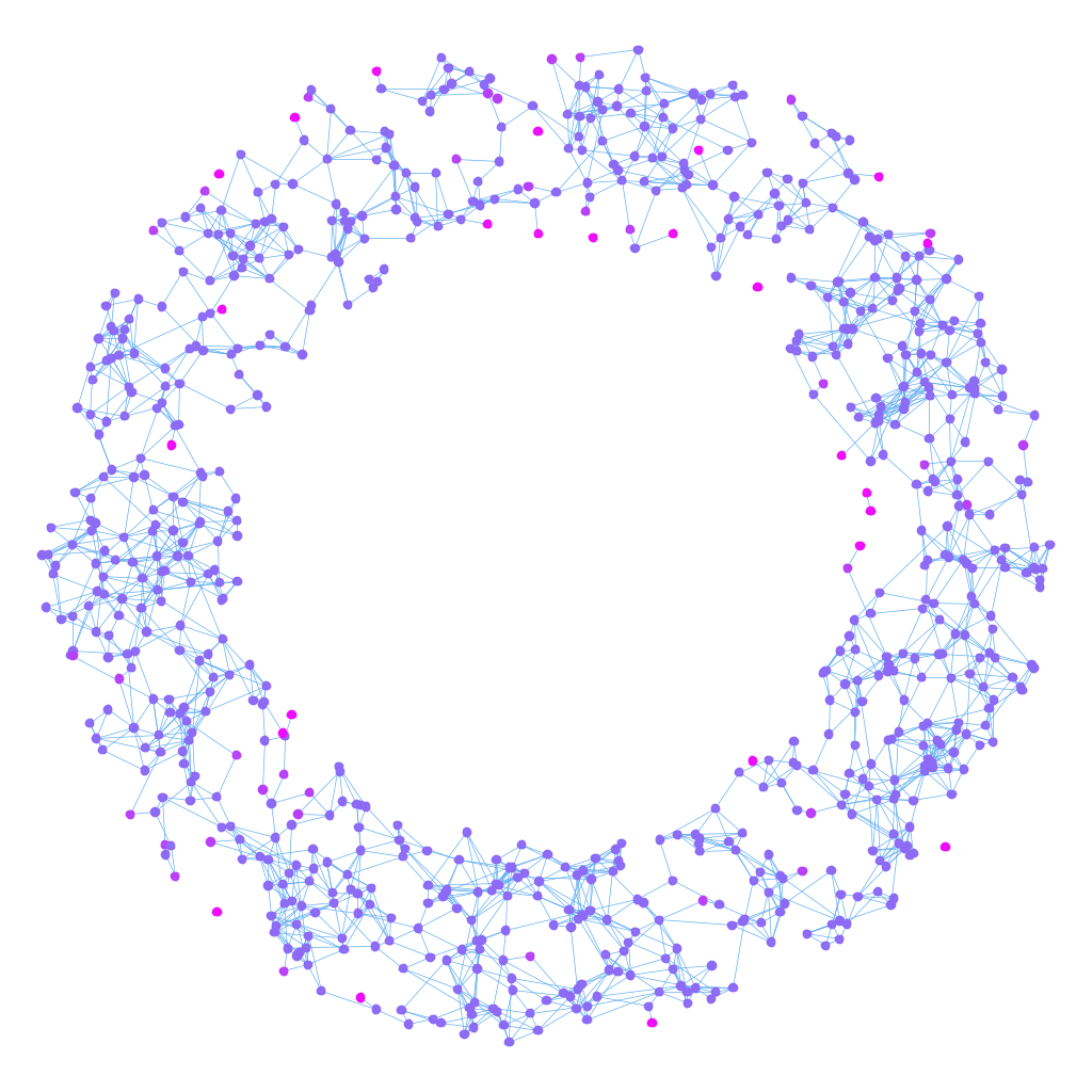
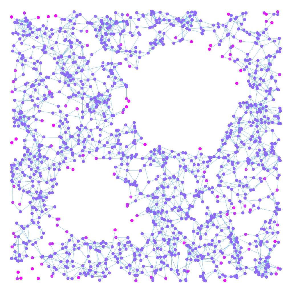
Figure 1: (Colour online) Randomly constructed soft geometric graphs (picked from the ensemble, with links formed based on the Rayleigh fading of electromagnetic data signals and nodes configured randomly) drawn inside $\mathcal{{A}}$ (left) and a square domain (right) containing two circular obstacles. Nodes with only a few connections (usually near the domain edges) are highlighted in purple, demonstrating the boundary effect phenomenon.

II Soft random geometric graphs bounded within non-convex geometries

Let $\mathcal{V}\subseteq\mathbb{R}^{d}$ be a bounded region of volume $V$ associated with both the Lesbegue measure $\mathrm{d}x$ and the Euclidean metric $r_{xy}=\lVert x-y\rVert$ for any $x,y\in\mathcal{V}$. We define the characteristic function

$$\chi\left(x,y\right)=\begin{cases}1&\quad\text{if }x+\lambda\left(y-x\right)\in\mathcal{V}\text{ for all }\lambda\in\left[0,1\right]\\ 0&\quad\text{otherwise}\\ \end{cases}$$ (II.1)

implying that $\mathcal{V}$ is a convex set whenever $\chi\left(x,y\right)=1$ for every pair $x,y\in\mathcal{V}$.

Let $\mathcal{Y}$ be a Poisson point process of intensity $\rho$ on $\mathcal{V}$ with respect to Lesbegue measure $\textrm{d}x$ on $\mathbb{R}^{d}$. Construct a soft random geometric graph in the following way: for every (unordered) pair of nodes $x,y\in\mathcal{Y}$, add an edge between $x$ and $y$ (independently for each pair) with probability $\chi\left(x,y\right)H\left(r_{xy}\right)$, where the measurable function $H:\mathbb{R}^{d}\to\left[0,1\right]$ is called the connection function. Should a node form $k$ links we say its has degree $k$, and call these linked nodes neighbours.

II.1 The degree distribution

Given that $\mathcal{Y}$ contains a point at $x\in\mathcal{V}$, the remaining points of $\mathcal{Y}$ are again distributed as a Poisson process of intensity $\rho$ on $\mathcal{V}$, by Palm theory for the Poisson process: see e.g. $\S 1.7$ of Penrose’s book penrosebook . So consider a vertex at some fixed $x\in\mathcal{V}$. We can determine its degree distribution by looking at a marked Poisson point process $\mathcal{Y}^{\star}$ constructed by adorning each $y\in\mathcal{Y}$ with an independent $U\left[0,1\right]$ random mark $u_{y}$, where $U\left[0,1\right]$ denotes the uniform distribution on the unit interval $\left[0,1\right]$. Then by the marking theorem for Poisson processes (see $\S 5.2$ of Kingman’s book kingmanbook ),

$$\mathcal{Y}^{\star}=\left\{\left(y,u_{y}\right):y\in\mathcal{Y}\right\}$$ (II.2)

is a Poisson point process on $\mathcal{V}\times\left[0,1\right]$ of intensity $\rho$ but now with respect to Lebesgue measure on $\mathbb{R}^{d+1}$. The mark $u$ on each marked point $(y,u)\in\mathcal{Y}^{\star}$ is used to determine connectivity of $y$ to $x$: if $u\leq\chi(x,y)H(r_{xy})$, then $y$ is joined to $x$ by an edge. The degree of $x$ is then distributed as

$$k\left(x\right)=\sum_{\left(y,u\right)\in\mathcal{Y}^{\star}}\mathbf{1}\{u<\chi\left(x,y\right)H\left(r_{xy}\right)\}$$ (II.3)

This representation for $k(x)$ as a sum over values of a measurable function $f$ of $(y,u)\in\mathcal{Y}^{\star}$ enables us to apply Campbell’s theorem (see $\S 3.2$ of Kingman’s book kingmanbook ) to obtain that $k(x)$ follows a Poisson distribution with mean

$$\mathbb{E}\left[k\left(x\right)\right]=\rho\int_{\mathcal{V}\times\left[0,1\right]}\mathbf{1}\{u<\chi\left(x,y\right)H\left(r_{xy}\right)\}\textrm{d}y\textrm{d}u=\rho\int_{\mathcal{V}}\chi\left(x,y\right)H\left(r_{xy}\right)\textrm{d}y$$ (II.4)

In particular, the probability that $x$ has degree zero is

$$\exp\left(-\rho\int_{\mathcal{V}}\chi\left(x,y\right)H\left(r_{xy}\right)\mathrm{d}y\right)$$ (II.5)

Following Penrose’s conjecture mentioned in Section I (and found as Theorem 2.1 in penrose2013 ), it is natural in light of Eq. II.5 to conjecture that as $\rho\to\infty$, the total number of isolated nodes is well approximated by a Poisson distribution with mean

$$\rho\int_{\mathcal{V}}\exp\left(-\rho\int_{\mathcal{V}}\chi\left(x,y\right)H\left(r_{xy}\right)\mathrm{d}y\right)\mathrm{d}x$$ (II.6)

In this limit, the usual situation is that the obstacle to connectivity is the presence of isolated nodes waltersreview , and so another reasonable conjecture is that as $\rho\to\infty$

$$\mathbb{P}\left(\text{graph is connected}\right) \approx\mathbb{P}\left(\text{no isolated nodes}\right)$$

$$\approx\exp\left(-\rho\int_{\mathcal{V}}e^{-\rho\int_{\mathcal{V}}\chi\left(x,y\right)H\left(r_{xy}\right)\mathrm{d}y}\mathrm{d}x\right)$$

$$\approx 1-\rho\int_{\mathcal{V}}e^{-\rho\int_{\mathcal{V}}\chi\left(x,y\right)H\left(r_{xy}\right)\mathrm{d}y}\mathrm{d}x$$ (II.7)

In the following article we evaluate this formula for various bounded, non-convex regions $\mathcal{V}$ in order to elucidate the specific effect of obstacles on high-density network connectivity. Our formulas are ‘semi-rigorous’ in that they are based on (at least) the above assumptions. Rigorous proof of any formulas herein presented (in a similar fashion to the work of Penrose) is deferred to a later study.

We also note that though we use the Poisson model for the point set $\mathcal{Y}$ throughout, our simulations (in Fig. 3) consider only the binomial model, where $N$ nodes are selected uniformly at random from $\mathcal{V}$. The two models are closely related when $\rho=N/V$, in which case the Poisson process is locally a good approximation to (what is called) the binomial point process of $N$ nodes kingmanbook .

II.2 Dense networks

It is important to highlight our scaling of density and volume. It is common to find asymptotic results for connectivity in the literature (see e.g. gupta1998 ), where points are drawn according to the usual Poisson process of intensity $\rho\textrm{d}x$ inside a square $S_{n}$ of area $n$. Then, with $\rho$ fixed, one studies the limit $n\to\infty$. This would represent the thermodynamic limit if the critical connection range $r$ were to remain independent of the geometry of the square, but it does not and instead we have $r\left(n\right)$ scaling in some way with the geometry.

Call graphs formed in this way $G\left(n,r\left(n\right)\right)$. One can then prove that, given some supercritical connection range

$$\lim_{n\to\infty}\mathbb{P}\left(G\left(n,r\left(n\right)\right)\textit{is connected}\right)=1$$ (II.8)

This critical scaling is known penrosebook to be of the order $r^{2}\left(n\right)\approx\log n$, beyond which we enter a phase where almost all graphs connect rather than almost all graphs do not connect. One is interested in the point in the parameter space at which this transition occurs.

But our random geometric graphs do not scale this way. The nodes connect according to a continuous function of their Euclidean separation, and we asymptotically scale the geometry-independent density of the point process $\rho\to\infty$. As has previously been noted cef2012 ; coon2012 , the enclosing boundary of $\mathcal{V}$ becomes the dominant influence on connectivity as density increases. We study a similar effect, but concerning convex obstacles, rather than the enclosing perimeter.

II.3 Rayleigh fading means soft connection

In ‘soft’ graphs, links are formed between nodes with a certain probability (such as according to a coin toss). This allows us to model inter alia data transmission in an environment where connection fails according to an activity known as signal fading, a simple example of which is Rayleigh fading sklar1997 ; tsebook .

The information outage probability $P_{out}$ (quantifying how often the signal’s distortion causes the decoding error at the receiver to fall below a threshold rate $\Upsilon$) is given in the Rayleigh model by

$$P_{out} = P\left[\log_{2}\left(1+\frac{P}{N_{0}}\hskip 1.42262pt\lVert h\rVert^{2}\right)<\Upsilon\right]$$ (II.9)

where $h$ is the channel gain and $P/N_{0}$ is the signal-to-noise ratio. Since the channel gain is a complex Gaussian process, its magnitude is Rayleigh distributed and so $\lVert h\rVert^{2}$ is exponentially distributed

$$H\left(r_{xy}\right) = 1-P\left[\lVert h\rVert^{2}<\frac{N_{0}\left(2^{\Upsilon}-1\right)}{P}\right]$$ (II.10)

$$= 1-P\left[\lVert h\rVert^{2}<\beta r_{xy}^{\eta}\right]$$

$$= e^{-\beta r^{\eta}_{xy}}$$

since the signal to noise ratio is related to the propagation distance $r_{xy}$ through $P=cr_{xy}^{\eta}$ where $\eta$ is the ‘path loss exponent’; we uniquely consider $\eta=2$ (free-space propagation). Thus $\beta=N_{0}\left(2^{\Upsilon}-1\right)/c$. We also use

$$r_{0}=\beta^{-1/\eta}$$ (II.11)

to signify the length scale over which nodes connect, since the exponent $\beta r_{xy}^{\eta}>1$ whenever $r_{xy}>r_{0}$ (and vice versa).

III The annulus domain $\mathcal{{A}}$

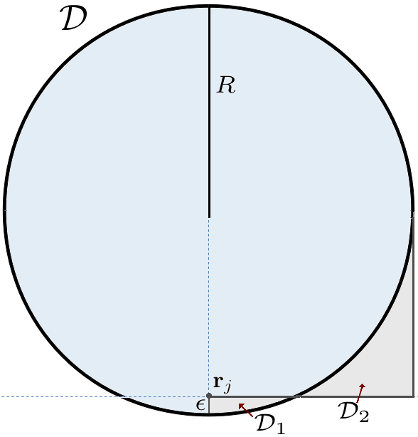
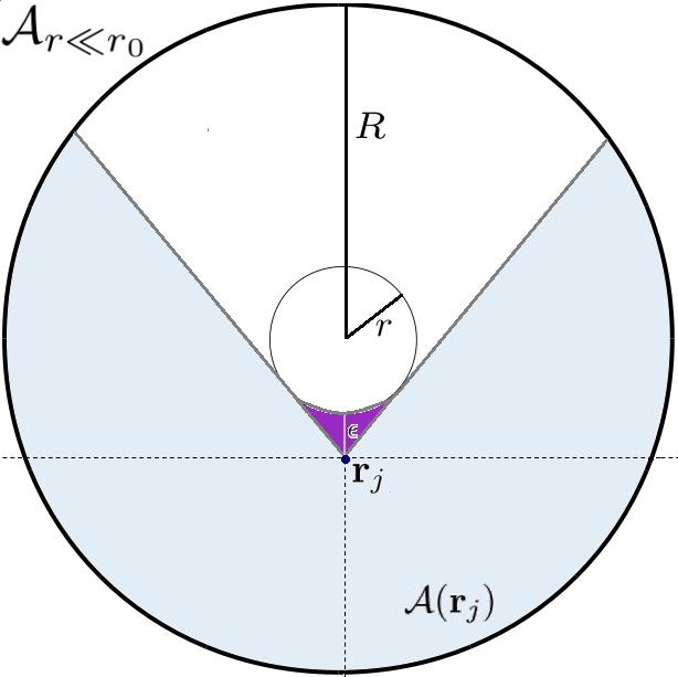
Figure 2: (Colour online) A depiction of the integration regions used for the disk domain $\mathcal{{D}}$ (left panel) and annulus domain $\mathcal{{A}}$ with small obstruction (middle panel) and large obstruction (right panel), with the integration regions highlighted. The small, cone-like region in the middle domain $\mathcal{A}$ is highlighted in purple.

In this section, we take $\mathcal{V}$ to be the annulus $\mathcal{{A}}$ of inner radius $r$ and outer radius $R\gg r_{0}$ (depicted in the left panel of Fig. 2). In order to simplify the necessary integrals, we define the ‘connectivity mass’ at $x\in\mathcal{A}$

$$\mathcal{M}\left(x\right) = \int_{\mathcal{A}}\chi\left(x,y\right)H\left(r_{xy}\right)\textrm{d}y$$ (III.1)

$$= \int_{\mathcal{A}\left(x\right)}H\left(r_{xy}\right)\textrm{d}y$$

(taken from the exponent in Eq. II.1). This is approximated within two obstacle-size regimes, the first where $r\ll r_{0}$, and the second where $r\gg r_{0}$; in each regime we can make some assumptions about the geometry of the region $\mathcal{A}\left(x\right)$ visible to $x$, which yields tractable formulas for the connectivity mass in terms of powers of the distance $\epsilon\in\left[0,R-r\right]$ from the obstacle perimeter. Given a slight correction to a previous result in cef2012 on connectivity within a disk of radius $R$, we then have $P_{fc}$ in $\mathcal{A}$.

III.1 No obstacles

We first take the case where $r=0$ depicted in Fig 2 (which is the disk $\mathcal{D}$). We quickly derive an approximation to $P_{fc}$ in this limiting domain (which we later extend into the annulus $\mathcal{A}$).

We first have the connectivity mass a distance $\epsilon$ from the disk’s centre, given by

$$\mathcal{{M}}\left(\epsilon\right) = \frac{\pi}{2\beta}+2\left(\int_{\mathcal{{D}}_{1}}e^{-\beta\left(x^{2}+y^{2}\right)}\textrm{d}y\textrm{d}x-\int_{\mathcal{{D}}_{2}}e^{-\beta\left(x^{2}+y^{2}\right)}\textrm{d}y\textrm{d}x\right)$$ (III.2)

$$= \frac{\pi}{2\beta}-2\int_{0}^{R}\int_{0}^{\epsilon-\sqrt{R^{2}-x^{2}}}e^{-\beta\left(x^{2}+y^{2}\right)}\textrm{d}y\textrm{d}x$$

since the integral over $\mathcal{{D}}_{1}$ cancels.

Thus consider two regimes for the distance $\epsilon$: in the first, where $\epsilon\approx R$ (close to the boundary), we can make the approximation $\exp\left({-\beta y^{2}}\right)\approx 1$, since the distances $y$ from the horizontal to the lower semi-circle in Fig. 1 will be small, so we can approximate the integral in Eq. III.2

$$\int_{0}^{R}\int_{0}^{\epsilon-\sqrt{R^{2}-x^{2}}}e^{-\beta\left(x^{2}+y^{2}\right)}\textrm{d}y\textrm{d}x \approx \int_{0}^{R}\int_{0}^{\epsilon-\sqrt{R^{2}-x^{2}}}e^{-\beta x^{2}}\textrm{d}y\textrm{d}x$$ (III.3)

$$= \frac{\sqrt{\pi}}{2\sqrt{\beta}}\epsilon-\int_{0}^{R}e^{-\beta x^{2}}\sqrt{R^{2}-x^{2}}\textrm{d}x$$

such that

$$\mathcal{{M}}(\epsilon\approx R)=\frac{\pi}{2\beta}-\frac{1}{R\sqrt{\beta}}\left(\frac{\sqrt{\pi}}{4\beta}\right)+\left(R-\epsilon\right)\sqrt{\frac{\pi}{\beta}}+\mathcal{O}\left(\left(R-\epsilon\right)^{2}\right)$$ (III.4)

after Taylor expanding Eq. III.3 for $\epsilon\approx R$, since it is in this regime that the main contribution to Eq. II.1 comes from.

For the other regime (where $\epsilon\ll R$)

$$\mathcal{{M}}(\epsilon\ll R) \approx \int_{0}^{2\pi}\int_{0}^{\infty}r^{\prime}e^{-\beta r^{\prime 2}}\textrm{d}r^{\prime}\textrm{d}\theta$$ (III.5)

$$= \pi/\beta$$ (III.6)

due to the exponential decay of the connectivity function, and so we have the probability of connection $P_{fc}$

$$P_{fc} \approx 1-\rho\int_{\mathcal{V}}e^{-\rho\int_{\mathcal{V}}\chi\left(x,y\right)H\left(r_{xy}\right)\mathrm{d}y}\mathrm{d}x$$ (III.7)

$$= 1-\rho\int_{0}^{2\pi}\int_{0}^{L^{+}}\epsilon\exp\left(-\frac{\rho\pi}{\beta}\right)\textrm{d}\epsilon\textrm{d}\theta$$

$$-\rho\int_{L^{+}}^{R}\exp\left(-\rho\left(\left(\frac{\pi}{2\beta}-\frac{1}{R\sqrt{\beta}}\left(\frac{\sqrt{\pi}}{4\beta}\right)\right)+\left(R-\epsilon\right)\sqrt{\frac{\pi}{\beta}}\right)\right)\epsilon\textrm{d}\epsilon\textrm{d}\theta$$

$$\approx 1-\pi R^{2}\rho e^{-\frac{\rho\pi}{\beta}}-2\pi R\sqrt{\frac{\beta}{\pi}}e^{-\frac{\rho}{\beta}\left(\frac{\pi}{2}-\frac{1}{R\sqrt{\beta}}\left(\frac{\sqrt{\pi}}{4}\right)\right)}$$

where $L^{+}$ is the point where the two mass approximations equate. This approaches equation Eq. 38 of reference cef2012 as $R\sqrt{\beta}\rightarrow\infty$, where the second term in the exponent of the final term in Eq. III.7 is a ‘curvature correction’ to the disk result in that report. Monte-Carlo simulations (where graphs are drawn from the graph-ensemble and enumerated should they connect), presented in Fig. 3 alongside our approximation in Eq. III.7, corroborate our formula and show an improvement on the result in cef2012 . The discrepancy at low density is expected since we only consider the probability of a single isolated node.

We also highlight the interesting composition III.7. There is a bulk term (whose coefficient is proportional to the area of $\mathcal{D}$) and a boundary term (proportional to the circumference of $\mathcal{D}$). This is discussed in greater detail in e.g. cef2012 , though we again emphasise the dominance of the boundary term as $\rho\to\infty$.

III.2 Small obstacles

We now take the case where $r\ll r_{0}$ (but not necessarily zero), and take the outer perimeter $R\gg r_{0}$. We make the approximation that the small cone-like domain $\mathcal{{A}}_{c}$ (making up a portion of the region visible $\mathcal{A}\left(x\right)$ to $x$ in the middle panel of Fig. 2) is only significantly contributing to the connectivity mass at small displacements $\epsilon$ from the obstacle, since at larger displacements it thins and the wedge-like region $\mathcal{A}\left(x\right)\setminus\mathcal{A}_{c}$ dominates. Practically, it is $\mathcal{{A}}_{c}$ that presents the main integration difficulties, so we approximate $H\left(r_{xy}\right)$ over this region where the radial coordinate $r^{\prime}\ll 1$, using $\exp{-\beta r_{xy}^{\prime 2}}\approx 1$

$$\mathcal{M}\left(\epsilon\ll r_{0}\right) \approx \int_{-\pi+\arcsin\left(\frac{r}{r+\epsilon}\right)}^{\pi-\arcsin\left(\frac{r}{r+\epsilon}\right)}\int_{0}^{\infty}e^{-\beta r^{\prime 2}}r^{\prime}\textrm{d}r^{\prime}\textrm{d}\theta+2\int_{0}^{\arcsin\left(\frac{r}{r+\epsilon}\right)}\int_{0}^{\left(r+\epsilon\right)\cos(\theta)-\sqrt{r^{2}-\left(r+\epsilon\right)^{2}\sin^{2}(\theta)}}r^{\prime}\textrm{d}r^{\prime}\textrm{d}\theta$$ (III.8)

$$= \frac{1}{\beta}\left(\pi-\arcsin\left(\frac{r}{r+\epsilon}\right)\right)+\int_{0}^{\arcsin\left(\frac{r}{r+\epsilon}\right)}\left(\left(r+\epsilon\right)\cos\left(\theta\right)-\sqrt{r^{2}-\left(r+\epsilon\right)^{2}\sin^{2}\left(\theta\right)}\right)^{2}\textrm{d}\theta$$

$$= \frac{\pi}{\beta}+\left(r^{2}-\frac{1}{\beta}\right)\arcsin\left(\frac{r}{r+\epsilon}\right)+r\sqrt{2r\epsilon+\epsilon^{2}}-\frac{\pi}{2}r^{2}$$

For small $\epsilon$ (where the main contribution to Eq. II.1 is found) we have

$$\mathcal{M}\left(\epsilon\ll r_{0}\right)=\frac{\pi}{2\beta}+\frac{\sqrt{2}}{\beta\sqrt{r}}\epsilon^{1/2}+\frac{8\beta r^{2}-5}{6\beta\sqrt{2}r^{3/2}}\epsilon^{3/2}+\mathcal{O}\left(\epsilon^{2}\right)$$ (III.9)

leaving us to integrate over the annulus

$$P_{fc} \approx 1-\rho\int_{\mathcal{{A}}}e^{-\rho\mathcal{{M}}\left(x\right)}\textrm{d}x$$ (III.10)

$$\approx 1-\rho\int_{0}^{2\pi}\int_{0}^{L^{-}}\left(r+\epsilon\right)\exp\left(-\rho\left(\frac{\pi}{2\beta}+\frac{\sqrt{2}}{\beta\sqrt{r}}\epsilon^{1/2}+\frac{8\beta r^{2}-5}{6\beta\sqrt{2}r^{3/2}}\epsilon^{3/2}\right)\right)\textrm{d}\epsilon\textrm{d}\theta$$

$$-\pi R^{2}\rho e^{-\frac{\rho\pi}{\beta}}-2\pi R\sqrt{\frac{\beta}{\pi}}e^{-\frac{\rho}{\beta}\left(\frac{\pi}{2}-\frac{1}{R\sqrt{\beta}}\left(\frac{\sqrt{\pi}}{4}\right)\right)}$$

$$\approx 1-2\pi\rho\int_{0}^{L^{-}}\left(r+\epsilon\right)e^{-\frac{\rho\pi}{2\beta}}e^{-\rho\frac{\sqrt{2}}{\beta\sqrt{r}}\epsilon^{1/2}}\left(1-\rho\frac{8\beta r^{2}-5}{6\beta\sqrt{2}r^{3/2}}\epsilon^{3/2}\right)\textrm{d}\epsilon-\pi R^{2}\rho e^{-\frac{\rho\pi}{\beta}}-2\pi R\sqrt{\frac{\beta}{\pi}}e^{-\frac{\rho}{\beta}\left(\frac{\pi}{2}-\frac{1}{R\sqrt{\beta}}\left(\frac{\sqrt{\pi}}{4}\right)\right)}$$

$$\approx 1-\pi r^{2}\frac{2\beta^{2}}{\rho}e^{-\frac{\rho\pi}{2\beta}}-\pi R^{2}\rho e^{-\frac{\rho\pi}{\beta}}-2\pi R\sqrt{\frac{\beta}{\pi}}e^{-\frac{\rho}{\beta}\left(\frac{\pi}{2}-\frac{1}{R\sqrt{\beta}}\left(\frac{\sqrt{\pi}}{4}\right)\right)}$$

where $L^{-}$ is the point where the connectivity mass in the bulk meets our approximation $\mathcal{M}\left(\epsilon\ll r_{0}\right)$ near the obstacle. We numerically corroborate Eq. III.10 in Fig. 3 using Monte Carlo simulations.

Note that this obstacle term is extremely small compared to the other contributions in Eq. III.10, given its coefficient decays linearly with $\rho$ and the factor of $\left(r\sqrt{\beta}\right)^{2}\ll 1$. We conclude that a small internal perimeter of radius $r$ in any convex domain $\mathcal{V}$ results in a negligible effect on connectivity.

III.3 Large obstacles

For the large obstacle case ($r\gg r_{0}$)

$$\mathcal{M}\left(\epsilon\ll r_{0}\right) \approx 2\int_{0}^{\infty}\int_{0}^{\infty}e^{-\beta(x^{2}+y^{2})}\textrm{d}x\textrm{d}y+\int_{-\infty}^{\infty}\int_{0}^{\epsilon+\frac{1}{2r}x^{2}}e^{-\beta(x^{2}+y^{2})}\textrm{d}y\textrm{d}x$$

$$= \frac{\pi}{2\beta}+\frac{\sqrt{\pi}}{2\sqrt{\beta}}\int_{-\infty}^{\infty}e^{-\beta x^{2}}\textrm{erf}\left[\left(\epsilon+\frac{1}{2r}x^{2}\right)\sqrt{\beta}\right]\textrm{d}x$$

yielding a power series in $\epsilon$

$$\mathcal{M}\left(\epsilon\ll r_{0}\right) \approx \frac{\pi}{2\beta}+\frac{\pi}{2\beta}\textrm{erf}\left[\sqrt{\beta}\epsilon\right]+\frac{1}{r\sqrt{\beta}}\left(\frac{\sqrt{\pi}}{4\beta}e^{-\beta\epsilon^{2}}\right)$$ (III.12)

$$= \frac{\pi}{2\beta}+\frac{1}{r\sqrt{\beta}}\left(\frac{\sqrt{\pi}}{4\beta}\right)+\frac{\sqrt{\pi}}{\sqrt{\beta}}\epsilon+\mathcal{O}\left(\epsilon^{3/2}\right)$$

This implies the connectivity mass is scaling in the same way as for the outer boundary, but where the curvature correction (in the exponent of the last term in Eq. III.10) is of opposite sign. We therefore have

$$P_{fc}\approx 1-2\pi r\sqrt{\frac{\beta}{\pi}}e^{-\frac{\rho}{\beta}\left(\frac{\pi}{2}+\frac{1}{r\sqrt{\beta}}\left(\frac{\sqrt{\pi}}{4}\right)\right)}-\pi R^{2}\rho e^{-\frac{\rho\pi}{\beta}}-2\pi R\sqrt{\frac{\beta}{\pi}}e^{-\frac{\rho}{\beta}\left(\frac{\pi}{2}-\frac{1}{R\sqrt{\beta}}\left(\frac{\sqrt{\pi}}{4}\right)\right)}$$ (III.13)

which is corroborated numerically in Fig. 3.

This implies that large obstacles behave like separate, internal perimeters. In the large-domain limit (where the node numbers go to infinity and the connection range is tiny compared to the large domain geometry), we can thus use

$$P_{fc}\approx 1-2\pi\left(R+r\right)\sqrt{\frac{\beta}{\pi}}e^{-\frac{\rho\pi}{2\beta}}-\pi(R^{2}-r^{2})\rho e^{-\frac{\rho\pi}{\beta}}$$ (III.14)

IV The spherical shell $\mathcal{{S}}$

Consider now the spherical shell domain $\mathcal{{S}}$ of inner radius $r$ and outer radius $R$, which is the three-dimensional analogue of the annulus. We again ask for the connection probability $P_{fc}$.

IV.1 Small spherical obstacles

The region visible to the node at $x$ is again decomposed into two parts, the three-dimensional version of $\mathcal{{A}}_{c}$, called $\mathcal{{S}}_{c}$, and the rest of the region visible to $x$, denoted $\mathcal{{S}}(x)\setminus\mathcal{{S}}_{c}$. As in the annulus with the small obstacle, we approximate $H\left(r_{xy}\right)$ over this region where the radial coordinate $r^{\prime}\ll 1$ (which holds for $\epsilon\ll 1$ where the main contribution to the connectivity mass is found), using $\exp{-\beta r_{xy}^{\prime 2}}\approx 1$ such that the contribution to the connectivity mass over $\mathcal{M}_{\mathcal{S}_{c}}\left(\epsilon\right)$ is

$$\mathcal{M}_{\mathcal{S}_{c}}\left(\epsilon\right) = \int_{\mathcal{{S}}_{c}}r^{\prime 2}e^{-\beta r^{\prime 2}}\sin\theta\textrm{d}r^{\prime}\textrm{d}\theta\textrm{d}\varphi$$ (IV.1)

$$\approx \int_{\mathcal{{S}}_{c}}r^{\prime 2}\sin\theta\textrm{d}r^{\prime}\textrm{d}\theta\textrm{d}\varphi$$

We evaluate this by breaking up $\mathcal{{S}}_{c}$ into the area of a cone of radius $\lambda$, height $h$ and apex angle $2\theta_{c}$

$$\lambda = \frac{r}{r+\epsilon}\sqrt{2r\epsilon+\epsilon^{2}}$$ (IV.2)

$$h = \frac{2r\epsilon+\epsilon^{2}}{r+\epsilon}$$ (IV.3)

$$\theta_{c} = \arcsin\left(\frac{r}{r+\epsilon}\right)$$ (IV.4)

(with the apex at a distance $\epsilon$ from the obstacle), and the spherical segment (which on removal from the cone creates the shape of $\mathcal{S}_{c}$)

$$\mathcal{{M}}_{\mathcal{{S_{C}}}}\left(\epsilon\right) = \frac{1}{3}\pi\lambda^{2}h-\frac{1}{6}\pi\left(r+\epsilon-h\right)\left(3\lambda^{2}+\left(r+\epsilon-h\right)^{2}\right)$$ (IV.5)

$$= \frac{\epsilon^{2}\pi r^{2}\left(\epsilon+2r\right)^{2}}{3\left(\epsilon+r\right)^{3}}-\frac{\epsilon^{2}\pi r^{3}\left(2\epsilon+3r\right)}{3\left(\epsilon+r\right)^{3}}$$

$$= \frac{\epsilon^{2}\pi r^{2}}{3\left(\epsilon+r\right)}$$

Adding the mass over $\mathcal{{S}}\left(x\right)\setminus\mathcal{{S}}_{c}$, we use the fact that the full solid angle available to a bulk node is $4\pi$ and that the angle $\omega\leq\Omega$ available to the node at $x$ is

$$\omega = \frac{1}{4\pi}\int_{0}^{2\pi}\int_{0}^{\theta_{c}}\sin\left(\theta\right)\textrm{d}\theta\textrm{d}\varphi$$ (IV.6)

$$= \frac{1}{2}\left(1-\cos\left(\arcsin\left(\frac{r}{r+\epsilon}\right)\right)\right)$$

$$= \frac{1}{2}\left(1-\sqrt{1-\left(\frac{r}{r+\epsilon}\right)^{2}}\right)$$

such that

$$\int_{\mathcal{{S}}\left(x\right)\setminus\mathcal{{S}}_{c}}r^{\prime 2}e^{-\beta r^{\prime 2}}\sin\theta\textrm{d}r^{\prime}\textrm{d}\theta\textrm{d}\varphi=\frac{\pi\sqrt{\pi}}{\beta\sqrt{\beta}}\left(1-\frac{1-\sqrt{1-\left(\frac{r}{r+\epsilon}\right)^{2}}}{2}\right)$$ (IV.7)

We then have $\mathcal{{M}}\left(\epsilon\ll r_{0}\right)$

$$\mathcal{{M}}\left(\epsilon\ll r_{0}\right) \approx \frac{\epsilon^{2}\pi r^{2}}{3\left(\epsilon+r\right)}+\frac{\pi\sqrt{\pi}}{\beta\sqrt{\beta}}\left(1-\frac{1-\sqrt{1-\left(\frac{r}{r+\epsilon}\right)^{2}}}{2}\right)$$ (IV.8)

$$= \frac{\pi\sqrt{\pi}}{2\beta\sqrt{\beta}}+\frac{\pi\sqrt{\pi}}{\beta\sqrt{\beta}}\frac{1}{\sqrt{2r}}\epsilon^{1/2}+\frac{3\pi^{3/2}}{4\sqrt{2}\left(r\beta\right)^{3/2}}\epsilon^{3/2}+\mathcal{O}\left(\epsilon^{2}\right)$$ (IV.9)

which implies that small spherical obstacles reduce the connection probability within the unobstructed sphere domain $\mathcal{S}_{r=0}$ to give a connection probability of

$$P_{fc}^{\mathcal{S}_{r\ll r_{0}}} \approx P_{fc}^{\mathcal{S}_{r=0}}-\rho e^{-\rho\left(\frac{\pi\sqrt{\pi}}{2\beta\sqrt{\beta}}\right)}\int_{0}^{2\pi}\int_{0}^{\pi}\int_{0}^{L_{\mathcal{{S}}}^{-}}\left(r+\epsilon\right)^{2}\sin\left(\theta\right)e^{-\rho\left(\frac{\pi\sqrt{\pi}}{2\beta\sqrt{\beta}}+\frac{\pi\sqrt{\pi}}{\beta\sqrt{\beta}}\frac{1}{\sqrt{2r}}\epsilon^{1/2}+\frac{3\pi^{3/2}}{4\sqrt{2}\left(r\beta\right)^{3/2}}\epsilon^{3/2}\right)}\textrm{d}\epsilon\textrm{d}\theta\textrm{d}\varphi$$ (IV.10)

$$\approx P_{fc}^{\mathcal{S}_{r=0}}-\frac{4}{3}\pi r^{3}\left(\frac{12\beta^{3}}{\rho\pi^{3}}\right)e^{-\rho\left(\frac{\pi\sqrt{\pi}}{2\beta\sqrt{\beta}}\right)}$$

Figure 3: (Colour online) Monte Carlo simulations: We use Monte Carlo methods to estimate the connection probability of soft random geometric graphs drawn inside various annuli and spherical shells $\mathcal{A}$ and $\mathcal{S}$ respectively. Every curve is compared with our analytic predictions (darker line) from Eqs. III.7, III.10, III.13 and IV.14 (where indicated). The discrepancy at low density is expected due to the fact we calculate only the probability of a single isolated node, given the results in e.g. penrose2013 .

IV.2 Large spherical obstacles

For large obstacles ($r\gg r_{0}$), we extend Eq. III.3 into the third dimension. $\mathcal{M}\left(\epsilon\ll r_{0}\right)$ thus becomes

$$\mathcal{M}\left(\epsilon\ll r_{0}\right)\approx 4\int_{0}^{\infty}\int_{0}^{\infty}\int_{0}^{\infty}\textrm{d}x\textrm{d}y\textrm{d}ze^{-\beta(x^{2}+y^{2}+z^{2})}+\int_{-\infty}^{\infty}\int_{-\infty}^{\infty}\int_{0}^{\nu\left(x,z\right)}\textrm{d}y\textrm{d}x\textrm{d}ze^{-\beta(x^{2}+y^{2}+z^{2})}$$ (IV.11)

where $\nu\left(x,z\right)=\epsilon+\frac{1}{2r}\left(x^{2}+z^{2}\right)$, yielding

$$\mathcal{M}\left(\epsilon\ll r_{0}\right) \approx \frac{\pi\sqrt{\pi}}{2\beta\sqrt{\beta}}+\frac{\pi\left(r\sqrt{\beta\pi}\textrm{erf}\left[\epsilon\sqrt{\beta}\right]+e^{-\beta\epsilon^{2}}\right)}{2r\beta^{2}}$$ (IV.12)

$$= \frac{\pi\sqrt{\pi}}{2\beta\sqrt{\beta}}+\frac{\pi}{2\beta^{2}r}+\frac{\pi}{\beta}\epsilon+\mathcal{O}\left(\epsilon^{2}\right)$$

implying the connection probability is

$$P_{fc}^{\mathcal{S}_{r\gg r_{0}}} \approx P_{fc}^{\mathcal{S}_{r=0}}-\rho e^{-\rho\left(\frac{\pi\sqrt{\pi}}{2\beta\sqrt{\beta}}+\frac{\pi}{2\beta^{2}r}\right)}\int_{0}^{2\pi}\int_{0}^{\pi}\int_{0}^{L_{\mathcal{{S}}}^{-}}\left(r+\epsilon\right)^{2}\sin\left(\theta\right)\textrm{d}\epsilon\textrm{d}\theta\textrm{d}\varphi e^{-\rho\left(\frac{\pi}{\beta}\epsilon\right)}$$ (IV.13)

$$\approx P_{fc}^{\mathcal{S}_{r=0}}-4\pi r^{2}\left(\frac{\beta}{\pi}\right)e^{-\rho\left(\frac{\pi\sqrt{\pi}}{2\beta\sqrt{\beta}}+\frac{1}{R\sqrt{\beta}}\left(\frac{\pi}{2\beta\sqrt{\beta}}\right)\right)}$$

where $L^{-}$ is the point where our mass approximation in Eq. IV.12 is equal to the mass in the bulk of the sphere $\left(\pi/\beta\right)^{3/2}$ (given the argument used for the two-dimensional case in Eq. III.5).

We now have the connection probability in the spherical shell $\mathcal{S}$

$$P_{fc}^{\mathcal{S}}\approx 1-\frac{4\pi}{3}\left(R^{3}-r^{3}\right)\rho e^{-\rho\left(\frac{\pi\sqrt{\pi}}{\beta\sqrt{\beta}}\right)}-4\pi R^{2}\left(\frac{\beta}{\pi}\right)e^{-\rho\left(\frac{\pi\sqrt{\pi}}{2\beta\sqrt{\beta}}-\frac{1}{R\sqrt{\beta}}\left(\frac{\pi}{2\beta\sqrt{\beta}}\right)\right)}\\ -\begin{cases}\frac{4}{3}\pi r^{3}\left(\frac{12\beta^{3}}{\rho\pi^{3}}\right)e^{-\rho\left(\frac{\pi\sqrt{\pi}}{2\beta\sqrt{\beta}}\right)}&\quad\text{if }r\ll r_{0}\\ 4\pi r^{2}\left(\frac{\beta}{\pi}\right)e^{-\rho\left(\frac{\pi\sqrt{\pi}}{2\beta\sqrt{\beta}}-\frac{1}{R\sqrt{\beta}}\left(\frac{\pi}{2\beta\sqrt{\beta}}\right)\right)}&\quad\text{if }r\gg r_{0}\end{cases}$$ (IV.14)

which is corroborated numerically in Fig. 3 (but only for the large obstacle case, given the negligable size of the small obstacle term in comparison to the bulk and boundary contributions). Just as with the annulus, small spherical obstacles thus have little impact on connectivity, and large spherical obstacles behave like separate perimeters. This behaviour is likely the same for all dimensions $d>3$, where the geometry is a hypersphere containing a convex $d$-dimensional obstacle (which one might call a hyper-annulus).

V Scenarios where obstacle effects are dominant

In the previous sections, we have provided approximations for the probability of a single isolated node appearing within both the annulus $\mathcal{A}$ and spherical shell $\mathcal{S}$. We draw three main conclusions:

1. Small obstacles holes in the domain have little effect on connectivity (in all dimensions $d\geq 2$).
   

2. Large obstacles holes disrupt connectivity as separate domain boundaries (in all dimensions $d\geq 2$).
   

3. As $\rho\to\infty$, the effect of a convex obstacle of any size is quickly dominated by that of the enclosing perimeter (in all dimensions $d\geq 2$).

One may therefore be forgiven for suggesting that obstacles have little impact on connectivity in dense networks. This is not always true, and so in the next few subsections we highlight important situations where these convex obstructions are essential to connectivity, since the ‘small correction term’ provided by obstacle analysis in the dense network limit becomes (in some parameter regime) the dominant contribution to $P_{fc}$.

V.1 Multiple convex obstacles distributed over $\mathcal{V}$

Figure 4: (Colour online) Many obstacles: Taking the Sinai-like domain in Fig. 1 with side $L=100$ and containing $n$ circular obstacles of small radii $r=1$ (left-hand phase diagram) and large radii $r=6$ (right-hand phase diagram), we plot the ratio of the first term in Eq. V.2 with the sum of the components in Eq. V.1, whose magnitude is indicated by the color gradient on the respective legend. The obstacle effects dominate when this exceeds unity, highlighted by the dotted line on each graph. Also, the regions where $P_{fc}$ is (predicited by our formulas to be) below $4/5$ are faded to gray tones, indicating regions where our approximations to the connection probability begin to lose their accuracy. $\beta=1$ throughout.

Given that the holes are not too close, their effects add up in a linear fashion such that they potentially outweigh the effect of the boundary. To highlight this, take the Sinai-like domain in the right hand panel of Fig. 1. Without obstacles, we have

$$P_{fc}=1-L^{2}\rho e^{-\frac{\pi}{\beta}\rho}-4L\sqrt{\frac{\beta}{\pi}}e^{-\frac{\pi}{2\beta}\rho}-\frac{16\beta}{\rho\pi}e^{-\frac{\pi}{4\beta}\rho}$$ (V.1)

taken from cef2012 . This is composed of a bulk term, a boundary term and a corner term. As we have seen, introducing $n$ circular obstacles of various radii $r_{i}$ will reduce this connection probability such that we have

$$P_{fc}=1-\sum_{i=1}^{n}\pi r_{i}^{2}\left(\frac{2\beta^{2}}{\rho}\right)e^{-\frac{\rho\pi}{2\beta}}-\left(L^{2}-\sum_{i=1}^{n}\pi r_{i}^{2}\right)\rho e^{-\frac{\pi}{\beta}\rho}-4L\sqrt{\frac{\beta}{\pi}}e^{-\frac{\pi}{2\beta}\rho}-\frac{16\beta}{\rho\pi}e^{-\frac{\pi}{4\beta}\rho}$$ (V.2)

which holds whenever the obstacles are separated from each other and the boundary by at least $2r_{0}$. Fig. 4 presents two phase plot that demonstrate how the obstacle effects can become dominant given a certain number of obstacles $n$. As we pass through the moderate density regime, the obstacle effects pass through a phase of significance greater than the sum of the rest of the geometric contributions to $P_{fc}$ (i.e. the bulk, square perimeter and four corners).

V.2 Surfaces without boundary

Boundary effects can be removed by working on surfaces without an enclosing perimeter. Examples include the flat torus (popular in rigorous studies but difficult to realise in wireless networks), and the sphere. Thus as $\rho\to\infty$ the obstacle effects are the dominant contribution to $P_{fc}$.

This may be of interest to pure mathematicians studying random graphs for purposes outside communication theory penrosebook . Fractal obstacles may be of particular interest dettmann2014 .

V.3 Quasi-1D regime $r\approx R$

Note that as the width of the annulus goes to zero, the approximation used in Eq. II.1 (that connectivity is the same as no isolated nodes) breaks down. The graph now disconnects by forming two clusters separated from each other by two unpopulated strips of width usually greater than $r_{0}$. We call this situation (where $R\approx r$) the ‘quasi-1D’ regime, deferring its treatment to a later study. We emphasise that one-dimensional random geometric graphs are particularly interesting, since they provide a test-bed for other theories that may be difficult to study initially in dimensions $d\geq 2$.

VI Conclusions

We have derived semi-rigorous analytic formulas for the connection probability of soft random geometric graphs drawn inside various annuli and shells (of inner radius $r$ and outer radius $R$) given the link formation probability between two nodes is an exponentially decaying function of their Euclidean separation. This models the Rayleigh fading of radio signal propagation within a wireless ad hoc network.

We have thus extended the soft connection model into simple non-convex spaces based on circular or spherical obstacles (rather than fractal boundaries dettmann2014 , internal walls orestis2013 or fixed obstacles on a grid almiron2013 ). We highlight situations where obstacles are (and are not) important influences on connectivity:

1. Small obstacles have little impact on connectivity.
   

2. Large obstacles have a similar impact on connectivity as the enclosing perimeter, but their effects are dominated by the boundary as $\rho\to\infty$.

3. Multiple obstacles can have the dominant effect on connection within density regimes that are significant for various areas of application, particularly ad hoc communication networks deployed in urban environments. 5G wireless networks are an example of this scenario.

Further topics of study include the quasi one-dimensional regime, where connectivity is not governed by isolated nodes.

Understanding the connectivity of these spatially embedded graphs in non-convex domains is a crucial enabler for the reality of 5G wireless networks, particularly if these multi-hop relay systems form in cluttered, urban environments (which is likely). Limiting scenarios (such as ‘many obstacles’ and the ‘quasi-1D’ regime) prove to be particularly interesting.

Acknowledgements

The authors wish to thank Suzanne Binding and the directors of the Centre for Doctoral Training in Communications at the University of Bristol, alongside the directors of the Toshiba Telecommunications Research Laboratory (Europe) for their continued support. Thanks also go to the anonymous referee who suggested important clarifications to section II, and to the other referee for their very useful comments. They also thank Justin Coon, Tom Kealy, Leo Laughlin, Jon Keating and David Simmons for many helpful discussions.

References

• (1) M. D. Penrose, “Connectivity of soft random geometric graphs,” to appear in Ann. Appl. Probab., available at arXiv:1311.3897, 2013.
• (2) M. E. J. Newman, Networks: An Introduction. New York, NY, USA: Oxford University Press, 2010.
• (3) J. von Brecht, T. Kolokolnikov, A. Bertozzi, and H. Sun, “Swarming on random graphs,” J. Stat. Phys., vol. 151, no. 1-2, pp. 150–173, 2013.
• (4) S. Eubank, H. Guclu, V. S. A. Kumar, M. V. Marathe, A. Srinivasan, Z. Toroczkai, and N. Wang, “Modelling disease outbreaks in realistic urban social networks,” Nature, vol. 429, no. 6988, pp. 180–184, 2004.
• (5) M. Amin, “Energy: The smart grid solution,” Nature, vol. 499, no. 7457, pp. 145–147, 2013.
• (6) D. Tse and P. Viswanath, Fundamentals of Wireless Communication. Cambridge University Press, 2005.
• (7) G. Mao and B. D. Anderson, “On the Asymptotic Connectivity of Random Networks under the Random Connection Model,” INFOCOM, Shanghai, China, p. 631, 2011.
• (8) O. Georgiou, C. Dettmann, and J. Coon, “Network connectivity: Stochastic vs. deterministic wireless channels,” Proc. IEEE ICC 2014, Sydney, Australia, pp. 77–82, 2014.
• (9) M. Haenggi, J. Andrews, F. Baccelli, O. Dousse, and M. Franceschetti, “Stochastic geometry and random graphs for the analysis and design of wireless networks,” Selected Areas in Communications, IEEE Journal on, vol. 7, no. 27, pp. 1029–1046, 2009.
• (10) J. Li, L. Andrew, C. Foh, M. Zukerman, and H. Chen, “Connectivity, coverage and placement in wireless sensor networks,” Sensors, vol. 9, pp. 7664–7693, 2009.
• (11) C. K. Toh, Ad Hoc Mobile Wireless Networks: Protocols and Systems. Prentice Hall, 2001.
• (12) M. M. Halldórsson and T. Tonoyan, “How well can graphs represent wireless interference?,” Proc. Forty-Seventh Annual ACM Symposium on the Theory of Computing STOC ’15, pp. 635–644, 2015.
• (13) J. Coon, C. Dettmann, and O. Georgiou, “Full connectivity: Corners, edges and faces,” J. Stat. Phys., vol. 147, no. 4, pp. 758–778, 2012.
• (14) O. Georgiou, C. Dettmann, and J. Coon, “Connectivity of networks with general connection functions,” preprint available at arXiv:1411.3617, 2014.
• (15) B. Clark, C. Colbourn, and D. Johnson, “Unit disk graphs,” Discrete Mathematics, vol. 86, no. 1–3, pp. 165–177, 1991.
• (16) P. Erdős and A. Rényi, “On random graphs,” in Publ. Math. Debrecen, vol. 6, pp. 290–297, 1959.
• (17) G. Gilbert, “Random plane networks,” SIAM J., vol. 9, no. 4, pp. 533–543, 1961.
• (18) O. Georgiou, C. Dettmann, and J. Coon, “Network connectivity through small openings,” Proc. ISWCS ’13, Ilmenau, Germany, pp. 1–5, 2013.
• (19) A. P. Giles, O. Georgiou, and C. P. Dettmann, “Betweenness centrality in dense random geometric networks,” Proc. IEEE ICC 2015, London, UK, 2015.
• (20) M. G. Almiron, O. Goussevskaia, A. A. Loureiro, and J. Rolim, “Connectivity in obstructed wireless networks: From geometry to percolation,” in Proceedings of the Fourteenth ACM International Symposium on Mobile Ad Hoc Networking and Computing, Bangalore, India, pp. 157–166, 2013.
• (21) O. Georgiou, M. Z. Bocus, M. R. Rahman, C. P. Dettmann and J. P. Coon, “Keyhole and reflection effects in network connectivity analysis,” IEEE Commun. Lett. vol. 19, no. 3, pp. 427–430, 2015.
• (22) C. P. Dettmann, O. Georgiou, and J. P. Coon, “More is less: Connectivity in fractal regions,” Proc. IEEE ICC 2015, London, UK, 2015.
• (23) J. P. Coon, O. Georgiou, and C. P. Dettmann, “Connectivity in dense networks confined within right prisms,” 12th International Symposium on Modeling and Optimization in Mobile, Ad Hoc, and Wireless Networks, WiOpt 2014, Hammamet, Tunisia, 2014.
• (24) J. F. C. Kingman, Poisson Processes. Oxford University Press, 1993.
• (25) M. Walters, “Random Geometric Graphs,” in Surveys in Combinatorics 2011 (Robin Chapman, ed.), Cambridge University Press, 2011.
• (26) P. Gupta and P. R. Kumar, “Critical power for asymptotic connectivity,” in Proc. 37th IEEE Conference on Decision and Control, Tampa, Florida, vol. 1, pp. 1106–1110, 1998.
• (27) M. D. Penrose, Random Geometric Graphs. Oxford University Press, 2003.
• (28) J. Coon, C. Dettmann, and O. Georgiou, “Impact of boundaries on fully connected random geometric networks,” Phys. Rev. E, vol. 85, 011138, 2012.
• (29) B. Sklar, “Rayleigh fading channels in mobile digital communication systems. Part I: Characterization,” IEEE Communications Magazine, vol. 35, no. 7, 1997.