Nonlinear forecasting of the generalised Kuramoto-Sivashinsky equation

Abstract

We study the emergence of pattern formation and chaotic dynamics in the one-dimensional (1D) generalized Kuramoto-Sivashinsky (gKS) equation by means of a time-series analysis, in particular a nonlinear forecasting method which is based on concepts from chaos theory and appropriate statistical methods. We analyze two types of temporal signals, a local one and a global one, finding in both cases that the dynamical state of the gKS solution undergoes a transition from high-dimensional chaos to periodic pulsed oscillations through low-dimensional deterministic chaos with increasing the control parameter of the system. Our results demonstrate that the proposed nonlinear forecasting methodology allows to elucidate the dynamics of the system in terms of its predictability properties.

1 Introduction

The emergence of complex spatiotemporal behavior in spatially extended systems (SES) as a result of several mechanisms nonlinearly interacting with each other has attracted a lot of attention over the last few decades (see e.g. Cross & Hohenberg [1993]; Knobloch [2008]; Houghton et al. [2010]). A well-known example of SES is the Kuramoto-Sivashinsky (KS) equation:

$$\frac{\partial u}{\partial t}+u\frac{\partial u}{\partial x}+\frac{\partial^{2}u}{\partial x^{2}}+\nu\frac{\partial^{4}u}{\partial x^{4}}=0$$ (1)

where $\nu$ is a viscosity damping parameter. This equation is one of the simplest prototypes exhibiting spatiotemporal chaos that retains some of the basic ingredients of any nonlinear SES, namely instability/energy production ($\partial^{2}u/\partial x^{2}$), stability/energy dissipation ($\partial^{4}u/\partial x^{4}$), and nonlinearity ($u\partial u/\partial x$) that transfers energy from low to high wave numbers.

Equation (1) was first derived in the contexts of phase turbulence in reaction-diffusion systems Kuramoto & Tsuzuki [1976], wrinkled flame front propagation Sivashinsky [1977] and unstable drift waves driven by electron collision in a tokamak LaQuey et al. [1975]. Subsequently, it has been shown to be applicable in a wide spectrum of physical settings, including hydrodynamic (e.g. thin-film) instabilities Shivashinsky & Michelson [1980]; Babchin et al. [1983]; Hooper & Grimshaw [1985] and optics such as bright spots formed by self-forcing of the beam profile Munkel & Kaiser [1996]. For thin film flows in particular, such as falling films, the KS equation is obtained via a weakly nonlinear expansion of the 1D Navier-Stokes equations subject to wall and free-surface boundary conditions and assuming strong surface tension effects–long waves Homsy [1974] (derived before Kuramoto’s paper). Not surprisingly, understanding the dynamical behavior of the KS solution has been a major topic of research. For example, it has been shown that decreasing the viscosity damping coefficient $\nu$ in small system sizes with periodic boundary conditions leads to a transition from steady states to chaos through a period-doubling bifurcation process, which is known as Feigenbaum scenario Smyrlis & Papageorgiou [1991].

With the addition of dispersion, the KS equation becomes the gKS equation:

$$\frac{\partial u}{\partial t}+u\frac{\partial u}{\partial x}+\frac{\partial^{2}u}{\partial x^{2}}+\delta\frac{\partial^{3}u}{\partial x^{3}}+\nu\frac{\partial^{4}u}{\partial x^{4}}=0$$ (2)

where $\delta$ is a positive parameter that characterizes the relative importance of dispersion. This equation then embraces all elements of any nonlinear process that involves wave evolution in 1D, and has been reported in a wide variety of contexts, including a reactive falling film Trevelyan & Kalliadasis [2004], a film falling down a uniformly heated wall Kalliadasis et al. [2003] and a film falling down a vertical fiber Ruyer-Quil & Kalliadasis [2012] (see also the recent monograph Kalliadasis et al. [2012] for the derivation of the KS and gKS equations for thin-film flows), in step dynamics Sato & Uwaha [1994]; Misbah & Pierre-Louis [1996]; Sato et al. [1998]. An extended version that includes a non-local term has also been derived for conducting liquid film in the presence of an external electric field Tseluiko & Papageorgiou [2010].

It is now well-known that for small values of $\delta$ the dynamics of the gKS equation resembles the spatiotemporal chaotic behavior of the KS solution, while sufficiently large values of the dispersion parameter tend to arrest it in favor of spatially periodic travelling waves Kawahara [1983]. In a regime of moderate values of $\delta$ however, traveling waves or pulses appear to be randomly interacting with each other giving rise to what is widely known as weak/dissipative turbulence (in the “Manneville sense” Manneville [1985]; Kalliadasis et al. [2012]). The dynamics and interaction of such pulses have been studied extensively via e.g. coherent-structure theories Balmforth [1995]; Chang et al. [1995]; Ei & Ohta [1994]; Duprat et al. [2009]; Tseluiko et al. [2010b, a]; Duprat et al. [2011]; Tseluiko & Kalliadasis [2014] which have been extended to more involved equations Pradas et al. [2011a, 2012a] while the regularizing effects of dispersion have been considered by Chang et al. Chang et al. [1993], who constructed bifurcation diagrams for the periodic and solitary solutions of the gKS equation.

Hence, the gKS equation constitutes a paradigmatic model for the transition from chaotic to regular behaviour in spatially extended systems and as such it has been extensively analysed from a spatiotemporal analysis point of view (such transitions are nowadays relatively well-known) but it has not received attention from the point of view of pure temporal signal analysis. In fact, there is not up to date a detailed analysis of the chaotic properties of the gKS solution based on time-series tools (chaos theory), in particular nonlinear forecasting methodologies, and how dispersion affects e.g. its predictability properties (there are, on the other hand, several studies on the chaotic behavior of both the KS equation [e.g. Chian et al., 2002; Rempel & Chian, 2003] and a damped version of it [see e.g. Elder et al., 1997; Rempel et al., 2007]). We note that temporal signals are very often the only experimentally accessible data, hence the importance of understanding their dynamics and behaviour.

Chaos theory provides a comprehensive and systematic treatment of random-like complex dynamics in nonlinear systems arising from a broad spectrum of disciplines. Generally, a chaotic signal is defined in terms of the properties of exhibiting short-term predictability and long-term unpredictability, something which is a consequence of the strong dependence on the initial conditions. Therefore, given a temporal signal which describes a quantity of interest in the system, methodologies like nonlinear forecasting can be used to quantify many important invariants, such as the fractal dimension, Lyapunov exponents, and entropies for irregular temporal evolutions yielding a physical description of the corresponding dynamical structures and predictability properties of the system (see e.g. Casdagli [1989]; Abarbanel et al. [1993]; Baek et al. [2004]), with many important applications in e.g. weather prediction Patil et al. [2001]; Slingo & Palmer [2011] and transistor circuits Hanias et al. [2010].

Likewise, another related question of interest is whether the particular time series can be distinguished from being stochastic or chaotic Sugihara & May [1990]; Cazelles & Ferriere [1992]; Tsonis & Elsner [1992]. We note that stochastic effects are ubiquitous in many systems (see e.g. Lauritsen et al. [1996]; Nicoli et al. [2010]; Pradas et al. [2011b, 2012b] for a noisy version of the KS equation) and they may be present in any low-dimensional description of a nonlinear system, as the recent study on stochastic mode reduction of the KS equation using concepts from evolutionary renormalization group theory and information entropy indicates Schmuck et al. [2013a, b]. It is actually in this context that nonlinear forecasting methodologies become a valuable tool as the more traditional time-series analysis techniques, such as computing the power spectral density (PSD) or looking at the trajectories in the phase space, cannot distinguish between the two; it is noteworthy that both high-dimensional chaos and stochastic processes produce completely scattered plots in the phase space. Hence, providing a reliable and systematic technique that can answer these questions has received considerable attention over the years Guckenheimer [1982]; Gao et al. [2006]; Rosso et al. [2007]; Zunino et al. [2012].

In this work, we undertake a detailed study of the characteristics of the dynamical state of the gKS equation in a wide range of the parameter $\delta$ by making use of a time-series analysis based on chaos theory, and in particular a nonlinear forecasting method to extract the short-term predictability and long-term unpredictability characteristics of the gKS solution. We consider in particular two types of temporal signals, a local quantity, i.e. a single point in the system, and an appropriate global measure in the sense that is a spatially averaged quantity. We then apply several statistical and time-series methods, some of which are standard in chaos theory, but they have not been used to analyze the gKS solution, including the Lorenz return map and a nonlinear forecasting method. The latter in particular has recently been exploited in the context of a wide spectrum of chaotic systems such as experiments in propagating flame front instabilities induced by buoyancy/swirl coupling Gotoda et al. [2010] and thermoacoustic combustion instabilities in a gas-turbine model combustor Gotoda et al. [2011]. Other examples include numerical solutions of sets of nonlinear differential equations for modeling intermittent Rayleigh-Bénard convection subjected to magnetic force Gotoda et al. [2013], and modeling flame front instabilities induced by radiative heat loss Gotoda et al. [2012b] with emphasis on the treatment of irregular temporal time series data. This forecasting method is an appropriate extension of the algorithm proposed by Sugihara and May Sugihara & May [1990], in the sense that it allows us to quantify the short-term predictability and long-term unpredictability as a function of the prediction time by taking into account the update of the library data in the phase space. This is crucial in order to understand the predictability properties of the system.

We find that as the parameter $\delta$ is increased both local and global quantities undergo a transition from high-dimensional chaos, characterized by scattered graphs in the phase space and a very short predictability time, to a periodic solution which can be predicted up to long times. At moderate values of $\delta$ the solution exhibits low-dimensional chaos and is characterized by a critical predictability time that we directly relate to the dispersion parameter $\delta$. We also compare the results from the gKS equation to pure stochastic processes like fractional Brownian motion to infer conditions under which the methodology can distinguish between the gKS signal from pure stochastic signals.

Section 2 presents the different dynamical states observed in the gKS equation as the dispersion parameter is increased and we define there the two temporal signals mentioned earlier. Section 3 briefly details the nonlinear forecasting method and Sec. 4 outlines the difference between a pure stochastic process and a deterministic chaotic signal. The results for the local and global analysis are presented in Sec. 5, Sec. 6, and Sec. 7. We finally conclude in Sec. 8.

2 Spatiotemporal dynamics of the gKS equation

Consider the gKS equation (2) in a domain $[-L,L]$, i.e. of size $2L$, with periodic boundary conditions and discretized into $N_{L}$ points. We choose random initial conditions $u(x,0)=\xi(x)$ where $\xi(x)$ is a spatial white noise with $\langle\xi(x)\xi(x^{\prime})\rangle=2\delta(x-x^{\prime})$. The numerical solution $u(x,t)$ is obtained by adopting a pseudo-spectral method for the spatial derivatives that uses the Fast Fourier Transform (FFT) to transform the solution to Fourier space. The nonlinear terms are evaluated in real space and transformed back to Fourier space by using the inverse FFT. The solution is then propagated in time by making use of a modified fourth-order exponential time-differencing–time-stepping Runge-Kutta (ETDRK4) scheme Kassam & Trefethen [2005], which is very stable for stiff equations Shen et al. [2011]. It has been reported in previous studies Elder et al. [1997]; Wittenberg & Holmes [1999] that for sufficiently large $L$ many modes become active and the transition to spatiotemporal chaos in the KS equation becomes independent of $L$. On this basis we choose $L=500$ and $N_{L}$ = 5000. It is also important to emphasize that by taking a large number of discretised points (in our case $5000$) we ensure the probability density function of the random initial conditions converges to a Normal distribution of mean zero and variance one so that starting the computations with different random initial conditions has little influence on the dynamic solutions. Note that solutions with different means can be on the other hand mapped to each other via a Galilean transformation (see e.g. Tseluiko & Kalliadasis [2014] for the gKS equation and Coullet & Fauve [1995]; Malomed [1992] for other systems with this type of symmetry). We also choose the value $\nu=1$ and we vary the dispersion parameter $\delta$ from $0$ to $3$. Note also that to improve the numerical precision, all numerical results, when necessary, have been obtained after averaging over 10 different realizations of the initial conditions.

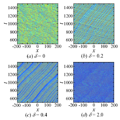
Figure 1: Spatiotemporal patterns of the gKS equation for the spatial and temporal regions of $x\in\left[-200,200\right]$ and $t\in\left[500,1500\right]$, respectively, and for different values of $\delta$. Different colours represent the magnitude of $u$ with high and low values in yellow and blue, respectively.

Figure 1 depicts spatiotemporal patterns of the gKS equation for different values of $\delta$. Clearly, for $\delta=0$, i.e., for the KS solution, the well-known spatiotemporal chaos is formed. As we increase $\delta$ up to $0.2$ localized coherent structures (solitary pulses) start to appear but with complicated chaotic dynamics due to their continuous interaction. Regularly-arrayed pulses with unsteady interpulse distances become predominant at $\delta$ = 0.4, and for sufficiently large $\delta$, i.e., in the dispersion-dominated regime, strongly regular structures with nearly constant interpulse distances are observed. These basic localized structures were firstly reported by Kawahara Kawahara [1983], and their dynamics and interactions have been extensively studied ever since Balmforth [1995]; Chang et al. [1995]; Ei & Ohta [1994]; Duprat et al. [2009]; Tseluiko et al. [2010b, a]; Tseluiko & Kalliadasis [2014].

2.1 Definition of local and global time series

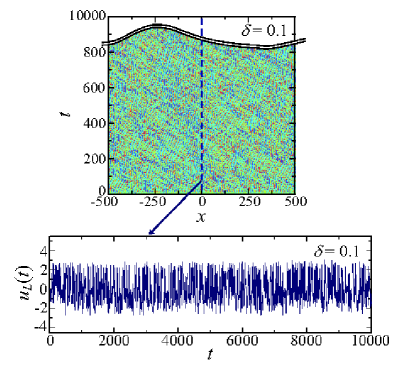
Figure 2: Extraction of the temporal evolutions of $u(x,t)$ at $x=0$ which defines the local magnitude $u_{L}(t)$ for the 1D gKS equation. Different colours represent the magnitude of $u$ with high values (yellow) and low values (blue).

We define here the magnitudes of interest which will be analyzed later on by means of several time-series tools to characterize the dynamics of the gKS solution as function of $\delta$. We distinguish between a local quantity, i.e. one that represents the dynamics of a single arbitrary point of the whole domain, and a global quantity as a spatially averaged measure that gives information of the global dynamics. We hence consider the temporal evolution of the gKS solution $u(x,t)$ located at $x=0$ and define our local time signal as:

$$u_{L}(t)\equiv u(0,t).$$ (3)

Note that this is actually a standard local quantity which has been used for example to characterize the dynamics of Turing patterns in a reaction-diffusion system Aragon et al. [2012]. Figure 2 shows the temporal evolution of $u_{L}$ for the case of $\delta=0.1$.

On the other hand, we define our global measure as the second moment of the gKS solution:

$$u_{G}(t)\equiv\frac{1}{2L}\int_{-L}^{L}[u(x,t)-\overline{u}(t)]^{2}\mathrm{d}x,$$ (4)

where the overbar denotes spatial average. This quantity has been considered in other settings, for example in the nonlocal gKS equation describing the interface evolution of conducting falling films Tseluiko & Papageorgiou [2010]. Our study will be based on how the dispersion (controlled via the parameter $\delta$) affects the dynamics of both the local $u_{L}$ and global $u_{G}$ quantities.

3 Nonlinear forecasting method

To study the predictability properties of the gKS equation we adopt a nonlinear forecasting methodology which is an appropriately extended version of the algorithm proposed by Sugihara and May Sugihara & May [1990], and it has been recently applied successfully in a wide spectrum of physical systems, from thermo-acoustic combustion instability Gotoda et al. [2011] to flame front instability induced by radiative heat loss Gotoda et al. [2012b] and intermittent behavior of Raylegh-Bénard convection subjected to magnetic force Gotoda et al. [2013]. The method proceeds as follows. Given a temporal signal, say $u(t)$, for $t\in[0,T_{f}]$, we divide it into two intervals, namely $t\in[0,t_{L}]$ and $t\in(t_{L},T_{f}]$, corresponding to a library and reference set of data, respectively. The values from the library data are used to predict the temporal evolution of $u(t)$ for $t>t_{L}$ which are then compared to the reference data.

We construct the phase space from the time series data based on Takens’ embedding theorem F.Takens [1981] by considering time-delayed coordinates, i.e. a vector in the phase space is given as:

$${\bf U}(t_{i})=(u(t_{i}),u(t_{i}-\tau),...,u(t_{i}-(D-1)\tau)),$$ (5)

where $i=1,\dots,n$ with $n$ the number of values in the data set, $D$ is the dimension of the phase space, and $\tau$ is a lag time which is estimated by making use of the mutual information proposed by Fraser & Swinney [1986], in a similar way as it was also done in Refs. Gotoda et al. [2012b, 2013]. In this study we set $D=3$ as we find it to be the optimal value which compromises numerical convergence (i.e. results do not change for larger values of $D$) and computational time (large values of $D$ become computationally expensive). We define ${\bf U}_{f}\equiv{\bf U}(t_{f})$ as the final point of a trajectory in the phase space, and ${\bf U}_{k}$, for $k=1\dots K$, its $K$ neighboring vectors which are searched from all data points in the phase space. The future value corresponding to ${\bf U}_{k}$ after some time $T=N\Delta t$ is denoted as $u(t_{k}+T)$, where $\Delta t$ is the sampling time of $u(t)$ and $N$ an arbitrary integer. The predicted value $\check{u}(t_{f}+T)$ from ${\bf U}_{f}$ is then obtained by a nonlinearly weighted sum of the library data $u(t_{k}+T)$ given as:

$$\check{u}(t_{f}+T)=\frac{\sum_{k=1}^{K}u(t_{k}+T)\mathrm{e}^{-d_{k}}}{\sum_{k=1}^{K}\mathrm{e}^{-d_{k}}},$$

where $d_{k}=\left\|{\bf U}(t_{f})-{\bf U}(t_{k})\right\|$. A comparison between the predicted value $\check{u}(t_{f}+T)$ and the reference value $u(t_{f}+T)$ is then quantified by looking at the standard correlation factor which is defined as:

$$C=\frac{\mathbb{E}[u(t)\check{u}(t)]}{\sigma_{u}\sigma_{\check{u}}},$$ (6)

where $\mathbb{E}[u(t)\check{u}(t)]$ represents the covariance between both signals, and $\sigma_{u}$ and $\sigma_{\check{u}}$ are the standard deviation of $u$ and $\check{u}$, respectively. It should be noted that our nonlinear forecasting method was developed in Refs. Gotoda et al. [2011, 2012b, 2013], where the temporal evolutions of $u$ are predicted by updating the library data and so we are able to capture the determinism of the system (with keeping the size of the updated library data constant). This point is actually the difference with the Sugihara-May algorithm Sugihara & May [1990] where the library data is not updated. In this sense, the correlation coefficient $C$ is estimated in terms of the duration $t_{P}$ of the actual temporal evolutions of $u$ added to the library data which is something that has not been proposed before for extracting the short-term predictability and long-term unpredictability characteristics of chaotic dynamics.

4 Chaotic versus stochastic behavior

Chaotic signals are characterized by exhibiting a high sensitivity on the initial conditions which in turn induces a decay of predictability in time. In particular, they exhibit short-term predictability and long-term unpredictability of the trajectories in the phase space, something which is referred to as orbital instability. A natural question of fundamental interest is then, given a time signal how can one distinguish between a pure deterministic chaotic signal from a stochastic process. Although in this work we focus on the deterministic gKS equation, we also analyze a stochastic signal by means of the nonlinear forecasting method which will be used in the subsequent sections for comparison with pure chaotic signals.

Consider the fractional Brownian motion which is a Gaussian process $B_{\alpha}(t)$ with zero mean, i.e. $\mathbb{E}[B_{\alpha}(t)]=0$, and a time dependent variance and covariance which are given as:

$$\mathbb{E}[B_{\alpha}(t)B_{\alpha}(t)] = t^{\alpha-1},$$ (7)

$$\mathbb{E}[B_{\alpha}(t)B_{\alpha}(s)] = (t^{\alpha-1}+s^{\alpha-1}-|s-t|^{\alpha-1})/2,$$ (8)

respectively, where $\alpha$ is the scaling exponent Mandelbrot & Ness [1968]. This is a well-known stochastic process model, the PSD of which exhibits a power-law behaviour of the type $1/f^{\alpha}$, describing irregular behavior in many areas of science and engineering Biagini et al. [2008]. On the other hand, the increment process defined as $\Delta B_{\alpha}\equiv B_{\alpha}(t_{i+1})-B_{\alpha}(t_{i})$ is fractional Gaussian noise. The particular case of $\alpha=5/3$ is referred to as a Gaussian Kolmogorov signal, in reference to the same type of PSD observed in fully-developed turbulence [see e.g. Vergassola et al., 1993; Katul et al., 2001]. For $\alpha=2$, it corresponds to Brownian motion, and the increment process is white noise.

To demonstrate the ability of the nonlinear forecasting methodology proposed in the preceding section for distinguishing chaos from stochastic process, we investigate the variations of the correlation coefficient $C$ in terms of the predicted time $t_{P}$ for the two representative cases of Brownian ($\alpha=2$) and fractional Brownian motion ($\alpha=5/3$) and the corresponding increment processes. We hence take $u(t)=B_{\alpha}(t)$ in Eq. (6) and compute the corresponding correlation coefficient for the two aforementioned values of $\alpha$. The results for both cases are shown in Fig. 3. We observe that $C(t_{P}=1)\sim 1$ in both cases and it decreases with $t_{P}$. This means that the one-step-ahead short-term prediction with high accuracy is feasible for Brownian/fractional Brownian motion. However, when we compute the increment process $\Delta B_{\alpha}$ the correlation factor is almost zero regardless of $t_{P}$, indicating that it cannot be predicted. As we will show in the following section, this is a distinctive feature of a pure stochastic process and will allow us to distinguish it from the deterministic chaos of the gKS equation.

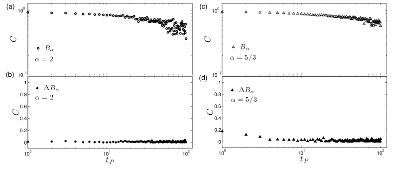
Figure 3: Correlation coefficient $C(t_{P})$ for (a) Brownian motion $B_{\alpha}(t)$ with $\alpha=2$ and the corresponding increment $\Delta B_{\alpha}(t)$ (b); and (c) fractional Brownian motion $B_{\alpha}(t)$ with $\alpha=5/3$ and the corresponding increment $\Delta B_{\alpha}(t)$ (d). Panels (a) and (c) are plots in log-log scale and panels (b) and (d) in semi-log scale.

5 Local analysis

5.1 Transition from chaotic to periodic solutions in the gKS equation

We start by studying how the dynamical state of the gKS solution undergoes the transition from a chaotic behavior, observed at low values of $\delta$, to a pulsating periodic dynamics which appears at sufficiently large values of $\delta$. To this end, we are going to perform a time-series analysis.

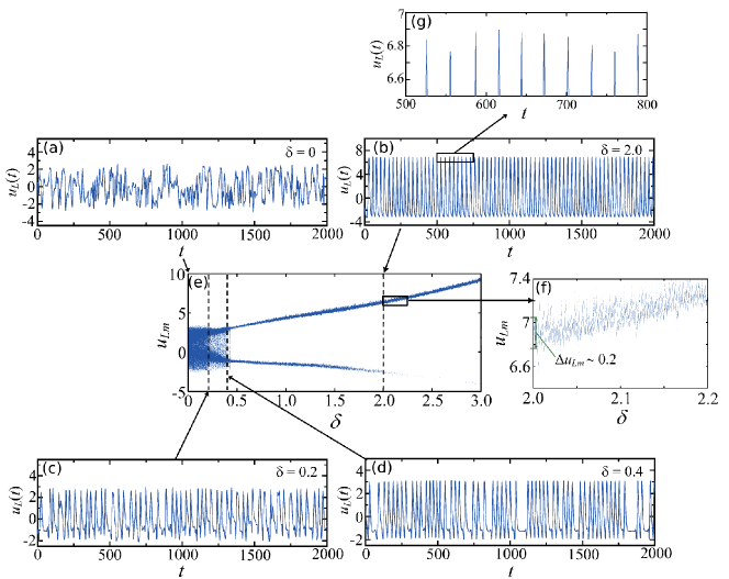
Figure 4: (a-d) Temporal evolutions of $u_{L}(t)$ for different values of $\delta$. (e) Bifurcation diagram of $u_{Lm}$. Panels (f) and (g) show a magnification of the selected area in panels (e) and (b), respectively.

5.1.1 Bifurcation diagram.

We look at the bifurcation diagram of the gKS equation by plotting the local maxima of the temporal signal $u_{L}(t)$ which we define as the values $u_{Lm}$ that satisfy the following condition:

$$u_{Lm}=\{u_{L}(t)\ :\ \dot{u}_{L}(t)=0,\ \ddot{u}_{L}(t)<0\}.$$ (9)

Temporal evolutions of $u_{L}(t)$ and the corresponding bifurcation diagram for different values of $\delta$ are shown in Fig. 4. We note that a repeated oscillation of $u_{L}(t)$ is displayed as a single point in the bifurcation diagram. We observe that $u_{L}(t)$ exhibits highly irregular fluctuations at $\delta=0$, which give rise in turn to the formation of uniformly distributed values of $u_{Lm}$ in the bifurcation diagram. For $\delta=0.2$, $u_{L}(t)$ starts to exhibit pulsating time fluctuations, and a hollow region appears in the bifurcation diagram around the values of $0\leq u_{Lm}\leq 2$. For $\delta\gtrsim 0.4$, these pulsating oscillations become more clear with temporal structures separated by irregular times, which leads to the appearance of two dominant branches in the bifurcation diagram. At this point the amplitude of the oscillating signal $u_{L}(t)$ is notably amplified as $\delta$ is increased which induces a gradual increase of the width separating the two branches in the bifurcation diagram.

In the dispersion-dominated region of $\delta\geq 2$, only the upper dominant branch persists, indicating the formation of strongly periodic pulsed oscillations. Note however that, as shown in the top right panel of Fig. 4, the pulsed amplitude is oscillating in time which is a consequence of the weak interaction between pulses. For larger values of $\delta$ such interactions would become weaker and a pure periodic signal would be recovered. It is important to point out that the main relevant change in the bifurcation diagram occurs at $\delta\sim 0.4$ where there is an indication of the onset of interior crisis. Several kind of crisis phenomena in the KS equation were found by Chian et al. [2002]; Rempel & Chian [2003], but there are no previous studies reporting the existence of such interior crisis in the temporal evolution of $u_{L}(t)$ for the gKS equation.

5.1.2 Power spectral density.

We analyze next the PSD of the signal $u_{L}(t)$ for different values of $\delta$ which is defined as

$$S_{u}(f)=\langle|\hat{u}_{L}(f)|^{2}\rangle,$$ (10)

where $\hat{u}_{L}(f)$ represents the Fourier transform in the frequency domain of $u_{L}(t)$ which is defined as $\hat{u}_{L}(f)=(1/\sqrt{T})\sum_{t}[u_{L}(t)-\overline{u}_{L}]\exp{(ift)}$, where $T$ is the time interval of observation and $\overline{u}_{L}$ is the mean value of the signal $u_{L}(t)$ over $T$. The symbols $\langle\dots\rangle$ in Eq. (10) denote average over different time intervals - we note that we are assuming statistically stationary solutions. Figure 5 shows that for $\delta\lesssim 0.2$ the PSD consists of a continuous distribution region at low frequencies followed by an exponential decay at higher frequencies. It is important to note that an exponential behaviour for the PSD is usually associated with deterministic chaotic systems (see e.g. Maggs & Morales [2011] and references therein) which indicates that the gKS solution is clearly chaotic for small values of $\delta$. For $\delta=0.4$ multiple peaks appear ($2f_{m}$, $3f_{m}$, $4f_{m}\dots$) with basic frequency $f_{m}=0.035$ corresponding to the temporal pulsating structures of $u_{L}(t)$ observed in Fig. 4, and indicate the multiple-periodicity nature of the signal. The appearance of these peaks becomes more prominent in the dispersion-dominated region of $\delta=2$.

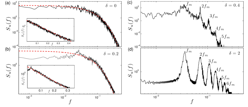
Figure 5: Log-log plot of the PSD $S_{u}(f)$ of $u_{L}(t)$ for different values of $\delta$. The insets in (a) and (b) correspond to a semi-log plot to show the exponential dependence. The dashed lines correspond to an exponential function $\exp{(-f\tau_{0})}$ with $\tau_{0}=33$ for $\delta=0$ (a) and $\tau_{0}=48$ for $\delta=0.2$ (b).

5.1.3 Dynamical structure of the phase space.

We compute the Lorenz return map which is obtained by plotting pairs of successive local maximum points, i.e. we define the $k$th local maximum as ${u_{Lm,k}}$ and we plot ${u_{Lm,k+1}}$ against ${u_{Lm,k}}$. Figure 6(a) depicts the results for $\delta=0$, $0.2$, $0.4$ and $2$. An entirely scattered structure appears for $\delta=0$, indicating the presence of chaotic behavior. For $\delta=0.2$ we get a map which is mainly gathered in three or four regions with scattered structures, which with increasing $\delta$ up to $0.4$, they progressively group in four main regions with locally scattered plots. Interestingly, two of them follow the straight line ${u_{Lm,k+1}}={u_{Lm,k}}$. In the dispersion-dominated regime with $\delta=2$, these four points aggregate at one region which belongs to the line ${u_{Lm,k+1}}={u_{Lm,k}}$. This is evidence of the formation of strongly periodic pulsating oscillations, but note that the group located at the top right of the map is still exhibiting a scattered structure. Note also that the amplitude of $u_{Lm}$ in Fig. 4 yields the entirely scattering plots in the localized region. This indicates that the dynamical state of $u$ at $\delta=2$ is dominated by a strongly periodic pulsed oscillation, but it involves small fluctuations in the oscillation amplitude (see top right panel of Fig. 4).

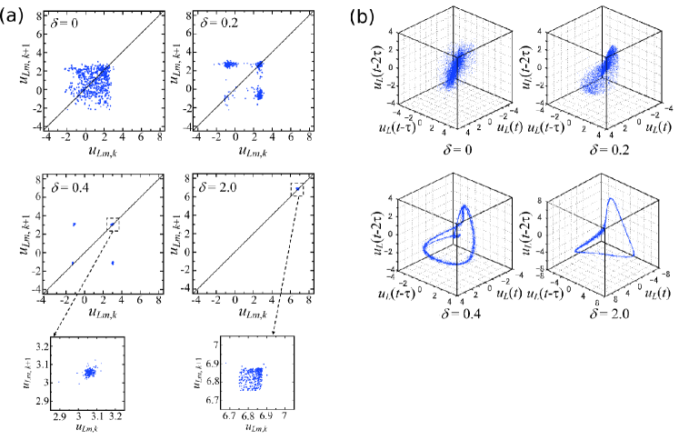
Figure 6: (a) Lorenz return map of $u_{L}(t)$ for different values of $\delta$. (b) 3D phase space $\left[u_{L}(t),u_{L}(t-\tau),u_{L}(t-2\tau)\right]$ for $\delta=0$ ($\tau=2$), $\delta=0.2$ ($\tau=2$), $\delta=0.4$ ($\tau=6$), and $\delta=2$ ($\tau=7$).

We also look at the three dimensional (3D) phase space which we construct by considering $\left[u_{L}(t),u_{L}(t-\tau),u_{L}(t-2\tau)\right]$. The results for different values of $\delta$ are plotted in Fig. 6(b). As before, we observe a entirely scattered graph for $\delta=0$ which fills the core of the attractor, indicating hence the presence of high-dimensional chaos. It still remains a scattered structure for $\delta=0.2$, but is different from that at $\delta=0$. The difference between the two cases is hard to be extracted by the conventional linear analysis such as the PSD (see Fig. 4). In this sense, drawings of the Lorenz return map and the 3D phase space are useful for capturing the subtle differences between the dynamical state of the KS and the gKS equation with small $\delta$. With $\delta$ increasing up to $0.4$ the overall shape of the attractor exhibits the geometrical structure of a strange attractor which is a consequence of the occurrence of multiple-periodic pulsed oscillations with irregular time intervals, indicating hence the presence of low-dimensional chaos. For $\delta=2$, we observe the emergence of a limit cycle with some small fluctuations corresponding to the fluctuating amplitude (see Fig. 4).

5.2 Nonlinear forecasting analysis

We apply the methodology described in Sec. 3 to study the predictability properties of $u_{L}(t)$. We divide the time series $u_{L}(t)$ into library and reference data by considering the values of $u_{L}$ up to $t_{L}=2500$ to be used as library data and those thereafter as reference data.

Figure 7(a) depicts the correlation coefficient $C$ as function of the prediction time $t_{P}$ for different values of $\delta$. We observe that for the KS equation ($\delta=0$), $C$ at $t_{P}=1$ is nearly unity, which means that one-step-ahead prediction of the dynamical state is feasible with high accuracy. However, $C$ decreases rapidly with $t_{P}$ reaching nearly zero at $t_{P}=100$. As $\delta$ is increased, we observe that a short plateau of constant $C$ starts to appear which, after a critical predicted time, say $t_{P,c}$, is followed by a rapid decay the rate of which depends on the particular value of $\delta$, and which can be approximated by a power-law tail, $C(t_{P})\sim t_{P}^{-\gamma}$, with the exponent $\gamma$ depending on $\delta$. In particular we find that

$$C(t_{P})\sim\left\{\begin{array}[]{l l}1&\quad\text{if $t_{P}<t_{P,c}$},\\ t_{P}^{-\gamma}&\quad\text{if $t_{P}>t_{P,c}$},\end{array}\right.$$ (11)

with $\gamma=0.67\pm 0.06$ for $\delta=0$, $\gamma=0.55\pm 0.07$ for $\delta=0.1$, and $\gamma=0.41\pm 0.04$ for $\delta\geq 0.2$. Based on the above relationship, the predicted critical time $t_{P,c}$ is hence numerically obtained by fitting a power law at long times and a constant function at short times, and find the point where these two behaviours meet [see the inlet panel of Fig. 7(b) for an example]. The fact that the same exponent $\gamma$ is observed for $\delta\geq 0.2$ suggests data of $C$ for different values of $\delta$ should collapse when plotted against the ratio $t_{P}/t_{P,c}$. The results are presented in Fig. 7(b), where we can observe an excellent data collapse indicating indeed that for $\delta\geq 0.2$ the exponent $\gamma$ becomes independent of $\delta$. Note that the appearance of such constant region followed by a rapid decrease is the manifestation of short-term predictability and long-term unpredictability characteristics of chaos which are separated by the critical value $t_{P,c}$. It is important to emphasize that even in the case of $\delta=0.4$, where the spatial solution is characterized by localized structures, the temporal behavior exhibits a chaotic motion which is a consequence of the irregular interaction between these structures. This regime corresponds to low-dimensional chaos, or what sometimes is referred to as weak/dissipative turbulence (in the “Manneville sense” Manneville [1985], as noted in the Introduction).

In the dispersion-dominated region with $\delta=2$, the region of constant $C$ becomes significantly larger followed by a slower decay. We note that if the dynamical state is periodic oscillations, $C$ is unity regardless of $t_{P}$ meaning a long-term predictability (see inlet panel of Fig. 7(a) for an example of temporal prediction of a sine wave $\sin{\left(2\pi ft\right)}$ with $f=0.035$). The gradual decay of the gradient of $C$ at $\delta=2$ is attributed to small fluctuations in pulsed oscillation amplitude extracted by the Lorenz return map, i.e. uniformly-scattered plots in a single region.

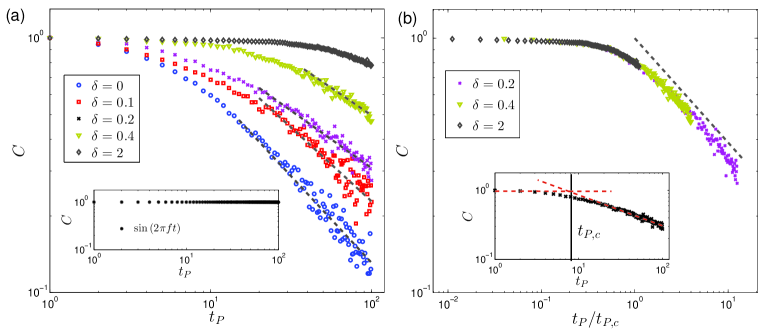
Figure 7: (a) Log-log plot of the time correlation coefficient $C(t_{P})$ for $u_{L}(t)$ against the predicted time $t_{p}$ for different values of $\delta$. The inlet panel corresponds to the correlation coefficient for a pure periodic function $\sin{(2\pi ft)}$. (b) Data collapse of $C$ against $t_{P}/t_{P,c}$ where $t_{P,c}$ is the critical predicted time after which $C$ starts to decay. The dashed line corresponds to a decaying power-law tail with exponent $-0.4\pm 0.03$. The inlet panel shows how the critical predicted time $t_{P,c}$ is defined.

We also scrutinize the increment process of $u_{L}$ which we define as $\Delta u_{L}\equiv u_{L}(t_{i+1})-u_{L}(t_{i})$. Figure 8 shows the correlation coefficient $C$ for $\delta=0$, $0.2$ and $0.4$, where we observe a similar trend as we did with the results for $u_{L}$ [cf. Fig. 7(a)]. We note that the behavior of $\Delta u_{L}$ is completely different to the one observed for the increment process of the fractional Brownian dynamics (see Fig. 3). This indicates that a way of distinguishing between chaos and pure stochasticity is by looking at the predictability properties of the increment process, as opposed of looking at the original signal - this is particularly true for high-dimensional chaos ($\delta=0$) as both signals exhibit a similar trend for $C(t_{P})$.

Based on these results, the short-term predictability and long-term unpredictability of the gKS equation are summarized in Fig. 9. As we increase $\delta$, the dynamical state is stabilized and the gradient of the correlation coefficient against the prediction time, i.e. the exponent $\gamma$, decreases. The degree of short-term predictability can then be roughly estimated by the critical prediction time $t_{P,c}$. Figure 10 shows this time and the exponent $\gamma$ as function of $\delta$, observing that $t_{P,c}$ gradually increases for $\delta\geq 0.2$ and $\gamma$ rapidly decreases for $\delta<0.2$ and remains constant around the value $0.4$ until $\delta\sim 1$, after which starts slowly decreasing. It should be pointed out however that for these large values of $\delta$, the power-law behaviour at long times (and in turn the exponent $\gamma$) is largely affected by cross-over effects: to find the truly power-law decay we would need to go to longer values of $t_{P}$. These three regimes are identified with the existence of high-dimensional spatiotemporal chaos at low values of $\delta$, low-dimensional chaos at moderate values, and periodic solutions at large values. These results demonstrate that the proposed nonlinear forecasting methodology allows us to fully characterize the dynamics of the system in terms of its predictability properties.

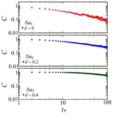
Figure 8: Correlation coefficient $C(t_{P})$ for the increment process $\Delta u_{L}(t)$ and for different $\delta$.

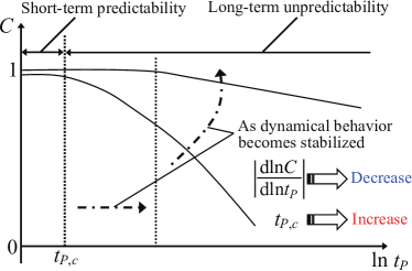
Figure 9: Schematic representation of short-term predictability and long-term unpredictability characteristics.

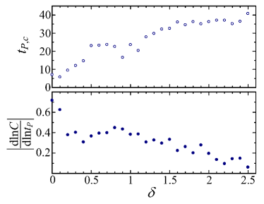
Figure 10: Variations in $t_{P,c}$ and $\gamma=|\mathrm{d}\ln C/\mathrm{d}\ln t_{P}|$ for $u_{L}(t)$ as a function of $\delta$. Typical errors are $3$ and $0.03$ for $t_{P,c}$ and $\gamma$, respectively.

6 Global analysis

We repeat the same analysis as in Sec. 5 but considering the global magnitude $u_{G}(t)$ as defined via the second moment in Eq. (4). Figure 11(a) depicts the temporal evolutions of $u_{G}(t)$ for different $\delta$. Irregular fluctuations are clearly formed for $\delta\lesssim 0.2$ and we now begin to observe some pulsating oscillations with irregular time interval separations at $\delta=0.4$ which become more regular at $\delta=2$. It is important to emphasize that in contrast to what we observed for the local magnitude $u_{L}$ [cf. Fig. 4], these pulsating oscillations are superimposed with a long wave oscillation of irregular frequency.

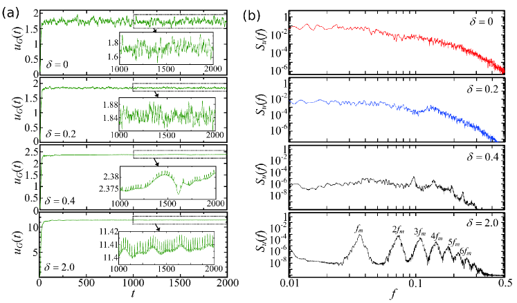
Figure 11: (a) Temporal evolutions of $u_{G}(t)$ for different $\delta$. (b) PSD of the global magnitude $u_{G}(t)$ for different $\delta$.

We compute the PSD of $u_{G}(t)$ observing a similar behavior as for the local magnitude $u_{L}$ when $\delta$ is increased [see Fig. 11(b)]. We also look at the Lorenz return map and the 3D phase space observing that now the transition from a completely scattered graph to structured graphs appears to be at larger $\delta$ values (see Fig. 12). Figure 13 shows the correlation coefficient $C$ for the signal $u_{G}$ and for the increment process $\Delta u_{G}\equiv u_{G}(t_{i+1})-u_{G}(t_{i})$, respectively. As before, we observe an initial regime of short-term predictability followed by a power-law decay of $C$ indicating the long-term unpredictability which is decreased as we increase $\delta$.

We note that the formation of periodic pulsed oscillations which are now superimposed on a long wave of irregular frequency (see Fig. 11 for $\delta=0.4$) makes the signal $u_{G}$ more chaotic as compared to $u_{L}$, in the sense that now the transition to long-term unpredictability appears before than in the case of $u_{L}$. This is more clear if we plot the critical predicted time $t_{P,c}$ against $\delta$, observing that now it increases until $\delta\sim 1.1$ after which it remains constant until $\delta=2.0$ (cf. Fig. 14). As for the gradient $|\mathrm{d}\ln C/\mathrm{d}\ln{t}_{P}|$, we observe that it initially decreases for $\delta\geq 0.2$ after which it remains constant until $\delta\sim 2$ for which it starts decreasing again. It is noteworthy that the critical predicted time is shorter than that for the local signal indicating hence that the global quantity appears to be less predictable.

7 Permutation entropy

Finally, we present an alternative analysis of both the local and global signals, $u_{L}$ and $u_{G}$, respectively, based on the concept of permutation entropy, which is an invariant measure of the complexity of the dynamics Bandt & Pompe [2002], and has been shown to be a good candidate to e.g. quantifying the dynamics in combustion instability Gotoda et al. [2012a]. This analysis complements the previous results and provides more information about the difference between the magnitudes of the local and global signals. A modified version of the permutation entropy has also been recently proposed to study heartbeat dynamics Bian et al. [2012].

The permutation entropy $h_{p}$ can be estimated by quantifying the degree of randomness from a sequence of ranks in the values of a time series. In particular, given a sequence with embedding dimension $D_{e}$, we index all possible permutations ($D_{e}!$) of order $D_{e}\geq 2$ as $\pi$. Each permutation represents a coarse-grained pattern of the dynamics when the sequence consists of $D_{e}$ successive data points taken from a time series. We first count the number of permutations denoted as $q(\pi)$ for all vectors ${\bf X}(t)=(u(t),u(t+1),\dots,u(t+D_{e}-1))$ consisting of sequences of order $D_{e}$. We then calculate the relative frequency for each permutation to obtain $p_{e}(\pi)=q(\pi)/(N-(D_{e}+1))$. We set $D_{e}=7$ in this study, and following the definition of Shannon entropy, $h_{p}$ is then calculated as:

$$h_{\mathit{p}}=\frac{-\sum\limits_{\pi}{p_{\mathit{e}}({\pi})}{\log_{2}}{p_{\mathit{e}}({\pi})}}{\log_{2}{D_{e}!}},$$ (12)

where $\log_{2}D_{e}!$ corresponds to the maximum permutation entropy and is used for normalization so that $0\leq h_{p}\leq 1$. Note that with this definition the lower bound ($h_{p}=0$) corresponds to a monotonically increasing or decreasing process, while the upper bound ($h_{p}=1$) corresponds to a completely random process.

Figure 19 shows the results of $h_{p}$ for both $u_{L}$ and $u_{G}$ as we change the values of $\delta$ from the high-dimensional chaos region ($\delta=0$) to the low-dimensional chaos region ($\delta=0.4$). We observe that $h_{p}$ decreases for both $u_{L}$ and $u_{G}$ with increasing $\delta$, as a consequence of the dispersion mechanism that arrests chaotic behavior. It is important to note that $h_{p}$ is significantly larger for the case of $u_{G}$, indicating that the dynamics of the global measure is more difficult to analyse than the corresponding local one, something which is a consequence of the averaging procedure.

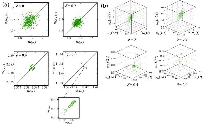
Figure 12: (a) Lorenz return map of $u_{G}(t)$ for different $\delta$. (b) 3D phase space of the global magnitude $u_{G}(t)$ for $\delta=0$ ($\tau=2$), $\delta=0.2$ ($\tau=2$), $\delta=0.4$ ($\tau=3$), and $\delta=2$ ($\tau=8$).

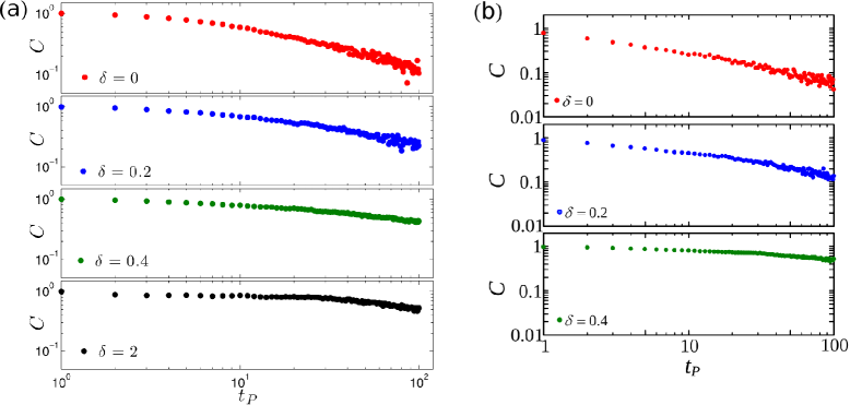
Figure 13: (a) Correlation coefficient $C(t_{P})$ of $u_{G}(t)$ (a) and $\Delta u_{G}(t)$ (b) for different values of $\delta$.

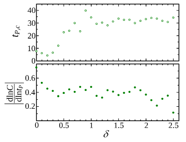
Figure 14: Variations of $t_{P,c}$ and $\gamma=|\mathrm{d}\ln C/\mathrm{d}\ln t_{P}|$ for $u_{G}(t)$ as a function of $\delta$. Typical errors are $4$ and $0.03$ for $t_{P,c}$ and $\gamma$, respectively.

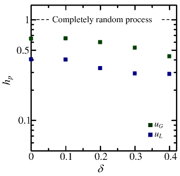
Figure 15: Variations of $h_{p}$ for $u_{L}$ and $u_{G}$ computed by using different values of $\delta$.

8 Conclusions

We have presented a detailed and systematic study of the dynamics of the spatiotemporal behavior of the gKS equation by making use of statistical methods and time-series analysis based on chaos theory, including a nonlinear forecasting method. The gKS equation is a generalization of the KS equation to include dispersion, and has been used as a prototype for the study of pattern formation dynamics and spatiotemporal complexity in active dispersive-dissipative media. The spatiotemporal solution of the gKS equation exhibits a rich dynamics that strongly depends on the parameter $\delta$ controlling the strength of the dispersion. In particular, one observes spatiotemporal chaos at low values of $\delta$, the emergence of localized structures (pulses) constantly interacting with each other at moderate values (regime also known as interfacial turbulence), and periodic solutions at large values of $\delta$.

We have defined two different temporal magnitudes to be analyzed: a local signal, the extracted solution in the middle of the system, and a global measure, the second moment of the solution. This allows for two different ways, a local and a global, of accessing the dynamical properties of the system providing then a complete picture (usually in experiments one has access to one of the two only). The local analysis has revealed that the high-dimensional chaos regime ($\delta\lesssim 0.2$) is characterized by a completely scattered graph in the phase space, a power-law decay PSD, and a very short predictability time. As the dispersion parameter is increased, the spatiotemporal solution starts to exhibit the emergence of solitary waves (pulses) which continuously and chaotically interact with each other. This corresponds to a low-dimensional chaos regime exhibiting a structured graph with a strange attractor in the phase space, and with a typical critical predictability time up to which the solution can be predicted. For larger values of $\delta$ the critical predictability time starts to increase as the solution approaches a periodic steady state ($\delta>1.8$).

We observe similar behavior for the global analysis but the transitions from high-dimensional to low-dimensional chaos and finally to periodic solutions occur at larger values of $\delta$, namely at $\delta\sim 1$ and $\delta\sim 2.0$, respectively. This is a consequence of the global spatial average we consider since any sign of localized structure is lost during such averaging procedure. In this sense we can conclude that the global measure is more chaotic than the local signal. This is also confirmed by looking at the permutation entropy of the temporal signals observing that the global signal has larger entropy than the local one.

We have also contrasted the results from the deterministic gKS equation to a pure stochastic process (fractional Brownian), observing that one needs to look at the increment process of the signal in order to distinguish between stochastic and high-dimensional chaotic signals. In particular, we have observed that while both the gKS solution at low values of $\delta$ and the fractional Brownian motion exhibit a very short predictability time for the original signal, the increment process shows zero predictability properties for the stochastic process and short predictability properties for the chaotic signal. To the best of our knowledge this is the first study to provide a comprehensive interpretation of the dynamical state of the gKS equation from the viewpoint of nonlinear forecasting.

Finally, there is a number of interesting questions related to the analysis presented here. For instance, how can one use elements from stochastic processes (e.g. in Krumscheid et al. [2013]) to appropriately modify the nonlinear forecasting method when the gKS equation is postulated for a nonlinear process for which the precise underlying model is not available. Another interesting problem would be the extension of the methodology proposed here to more involved equations, such as those describing the dynamics of the falling film away from criticality. We shall examine these and related issues in future studies.

Acknowledgments We thank Dr. G. A. Pavliotis and Prof. D. T. Papageorgiou for useful comments and suggestions. HG thanks the Department of Chemical Engineering of Imperial College for hospitality during a sabbatical visit. He was partially supported by a “Grant-in-Aid for Young Scientists (A)” from the Ministry of Education, Culture, Sports, Science and Technology of Japan (MEXT)” and from the JGC-S Scholarship Foundation. We acknowledge financial support from European Research Council (ERC) Advanced Grant No. 247031.

References

- Abarbanel et al. [1993] Abarbanel, H. D. I., Brown, R., Sidorowich, J. J. & Tsimring, L. S. [1993] “The analysis of observed chaotic data in physical systems,” Rev. Mod. Phys. 65, 1331.
- Aragon et al. [2012] Aragon, J. L., Barrio, R. A., Woolley, T. E., Baker, R. E. & Maini, P. K. [2012] “Nonlinear effects on turing patterns: Time oscillations and chaos,” Phys. Rev. E 86, 026201.
- Babchin et al. [1983] Babchin, A. J., Frenkel, A. L., Levich, B. G. & Sivashinsky, G. I. [1983] “Nonlinear saturation of Rayleigh-Taylor instability in thin films,” Phys. Fluids 26, 3159.
- Baek et al. [2004] Baek, S.-J., Hunt, B. R., Szunyogh, I., Zimin, A. & Ott, E. [2004] “Localized error bursts in estimating the state of spatiotemporal chaos,” Chaos 14, 1042–1049.
- Balmforth [1995] Balmforth, N. J. [1995] “Solitary waves and homoclinic orbits,” Annu. Rev. Fluid Mech. 27, 335.
- Bandt & Pompe [2002] Bandt, C. & Pompe, B. [2002] “Permutation entropy: A natural complexity measure for time series,” Phys. Rev. Lett. 88, 174102.
- Biagini et al. [2008] Biagini, F., Hu, Y., Øksendal, B. & Zhang, T. [2008] Stochastic Calculus for Fractional Brownian Motion and Applications (Springer Series on Probability and Its Applications, Springer-Verlag London).
- Bian et al. [2012] Bian, C., Qin, C., Ma, Q. D. Y. & Shen, Q. [2012] “Modified permutation-entropy analysis of heartbeat dynamics,” Phys. Rev. E 85, 021906.
- Casdagli [1989] Casdagli, M. [1989] “Nonlinear prediction of chaotic time series,” Physica D 35, 335.
- Cazelles & Ferriere [1992] Cazelles, B. & Ferriere, R. [1992] “How predictable is chaos?” Nature 355, 25–26.
- Chang et al. [1995] Chang, H.-C., Demekhin, E. & Kalaidin, E. [1995] “Interaction dynamics of solitary waves on a falling film,” J. Fluid Mech. 294, 123.
- Chang et al. [1993] Chang, H.-C., Demekhin, E. A. & Kopelevich, D. I. [1993] “Laminarizing effects of dispersion in an active-dissipative nonlinear medium,” Physica D 63, 299.
- Chian et al. [2002] Chian, A. C.-L., Rempel, E. L., Macau, E. E., Rosa, R. R. & Christiansen, F. [2002] “High-dimensional interior crisis in the Kuramoto-Sivashinsky equation,” Phys. Rev. E 65, 035203.
- Coullet & Fauve [1995] Coullet, P. & Fauve, S. [1995] “Propagative phase dynamics for systems with galilean invariance,” Phys. Rev. Lett. 55, 2857.
- Cross & Hohenberg [1993] Cross, M. & Hohenberg, P. [1993] “Pattern formation outside equilibrium,” Rev. Mod. Phys. 65, 851–1112.
- Duprat et al. [2009] Duprat, C., Giorgiutti-Dauphiné, F., Tseluiko, D., Saprykin, S. & Kalliadasis, S. [2009] “Liquid film coating a fiber as a model system for the formation of bound states in active dispersive-dissipative nonlinear media,” Phys. Rev. Lett. 103, 234501.
- Duprat et al. [2011] Duprat, C., Tseluiko, D., Saprykin, S., Kalliadasis, S. & Giorgiutti-Dauphiné, F. F. [2011] “Wave interactions on a viscous film coating a vertical fibre: Formation of bound states,” Chem. Eng. Process. 50, 519–524.
- Ei & Ohta [1994] Ei, S.-I. & Ohta, T. [1994] “Equation of motion for interacting pulses,” Phys. Rev. E 50, 4672.
- Elder et al. [1997] Elder, K. R., Gunton, J. D. & Goldenfeld, N. [1997] “Transition to spatiotemporal chaos in the damped Kuramoto-Sivashinsky equation,” Phys. Rev. E 56, 1631.
- Fraser & Swinney [1986] Fraser, A. M. & Swinney, H. L. [1986] “Independent coordinates for strange attractors from mutual information,” Phys. Rev. A 33, 1134.
- F.Takens [1981] F.Takens [1981] Dynamical Systems of Turbulence, Vol. 898 (Lecture Notes in Mathematics, Springer-Verlag Berlin Heidelberg).
- Gao et al. [2006] Gao, J. B., Hu, J., Tung, W. W. & Cao, Y. H. [2006] “Distinguishing chaos from noise by scale-dependent Lyapunov exponent,” Phys. Rev. E 74, 066204.
- Gotoda et al. [2012a] Gotoda, H., Amano, M., Miyano, T., Ikawa, T., Maki, K. & Tachibana, S. [2012a] “Characterization of complexities in combustion instability in a lean premixed gas-turbine model combustor,” Chaos 22, 043128.
- Gotoda et al. [2012b] Gotoda, H., Ikawa, T., Maki, K. & Miyano, T. [2012b] “Short-term prediction of dynamical behavior of flame front instability induced by radiative heat loss,” Chaos 22, 033106.
- Gotoda et al. [2010] Gotoda, H., Miyano, T. & Shepherd, I. G. [2010] “Experimental investigation on dynamic motion of lean swirling premixed flame generated by change in gravitational orientation,” Phys. Rev. E 81, 026211.
- Gotoda et al. [2011] Gotoda, H., Nikimoto, H., Miyano, T. & Tachibana, S. [2011] “Dynamic properties of combustion instability in a lean premixed gas-turbine combustor,” Chaos 21, 013124.
- Gotoda et al. [2013] Gotoda, H., Takeuchi, R., Okuno, Y. & Miyano, T. [2013] “Low-dimensional dynamical system for Rayleigh-Benard convection subjected to magnetic field,” J. Appl. Phys. 113, 124902.
- Guckenheimer [1982] Guckenheimer, J. [1982] “Noise in chaotic systems,” Nature 298, 358.
- Hanias et al. [2010] Hanias, M. P., Giannis, I. L. & Tombras, G. S. [2010] “Chaotic operation by a single transistor circuit in the reverse active region,” Chaos 20, 013105.
- Homsy [1974] Homsy, G. M. [1974] “Model equations for wavy viscous film flow,” Lect. Appl. Math 15, 191.
- Hooper & Grimshaw [1985] Hooper, A. P. & Grimshaw, R. [1985] “Nonlinear instability at the interface between two viscous fluids,” Phys. Fluids 28, 37.
- Houghton et al. [2010] Houghton, S. M., Knobloch, E., Tobias, S. M. & Proctor, M. R. E. [2010] “Transient spatio-temporal chaos in the complex Ginzburg-Landau equation on long domains,” Phys. Lett. A 374, 2030.
- Kalliadasis et al. [2003] Kalliadasis, S., Demekhin, E. A., Ruyer-Quil, C. & Velarde, M. G. [2003] “Thermocapillary instability and wave formation on a film falling down a uniformly heated plane,” J. Fluid Mech 492, 303.
- Kalliadasis et al. [2012] Kalliadasis, S., Ruyer-Quil, C., Scheid, B. & Velarde, M. G. [2012] Falling Liquid Films, Vol. 176 (Springer Series on Applied Mathematical Sciences, Springer-Verlag Berlin Heidelberg).
- Kassam & Trefethen [2005] Kassam, A. K. & Trefethen, L. N. [2005] “Fourth-order time-stepping for stiff PDEs,” SIAM J. Sci. Comput. 26, 1214.
- Katul et al. [2001] Katul, G., Vidakovic, B. & Albertson, J. [2001] “Estimating global and local scaling exponents in turbulent flows using discrete wavelet transformations,” Phys. Fluids 13, 241.
- Kawahara [1983] Kawahara, T. [1983] “Formation of saturated solitons in a nonlinear dispersive system with instability and dissipation,” Phys. Rev. Lett. 51, 381.
- Knobloch [2008] Knobloch, E. [2008] “Spatially localized structures in dissipative systems: open problems,” Nonlinearity 21, T45–T60.
- Krumscheid et al. [2013] Krumscheid, S., Pavliotis, G. A. & Kalliadasis, S. [2013] “Semi-parametric drift and diffusion estimation for multiscale diffusions,” SIAM J. Multiscale Model. Sim. 11, 442.
- Kuramoto & Tsuzuki [1976] Kuramoto, Y. & Tsuzuki, T. [1976] “Persistent propagation of concentration waves in dissipative media far from thermal equilibrium,” Prog. Theor. Phys. 55, 356.
- LaQuey et al. [1975] LaQuey, R. E., Mahajan, S. M., Rutherford, P. H. & Tang, W. [1975] “Nonlinear saturation of the trapped-ion mode,” Phy. Rev. Lett. 34, 391.
- Lauritsen et al. [1996] Lauritsen, K. N., Cuerno, R. & Makse, H. A. [1996] “Noisy Kuramoto-Sivashinsky equation for an erosion model,” Phys. Rev. E 54, 3577.
- Maggs & Morales [2011] Maggs, J. E. & Morales, G. J. [2011] “Generality of deterministic chaos, exponential spectra, and lorentzian pulses in magnetically confined plasmas,” Phys. Rev. Lett. 107, 185003.
- Malomed [1992] Malomed, A. [1992] “Patterns produced by a short-wave instability in the presence of a zero mode,” Phys. Rev. A 45, 1009.
- Mandelbrot & Ness [1968] Mandelbrot, B. B. & Ness, J. W. V. [1968] “Fractional brownian motions, fractional noises and applications,” SIAM Review 10, pp. 422–437.
- Manneville [1985] Manneville, P. [1985] Macroscopic Modeling of Turbulent Flows, Vol. 230 (Lecture Notes in Physics, Springer-Verlag Berlin Heidelberg).
- Misbah & Pierre-Louis [1996] Misbah, C. & Pierre-Louis, O. [1996] “Pulses and disorder in a continuum version of step-bunching dynamics,” Phys. Rev. E 53, R4318–R4321.
- Munkel & Kaiser [1996] Munkel, M. & Kaiser, F. [1996] “An intermittency route to chaos via attractor merging in the Laser-Kuramoto-Sivashinsky equation,” Physica D 98, 156.
- Nicoli et al. [2010] Nicoli, M., Vivo, E. & Cuerno, R. [2010] “Kardar-parisi-zhang asymptotics for the two-dimensional noisy Kuramoto-Sivashinsky equation,” Phys. Rev. E 82, 045202(R).
- Patil et al. [2001] Patil, D. J., Hunt, B. R., Kalnay, E., Yorke, J. A. & Ott, E. [2001] “Local low dimensionality of atmospheric dynamics,” Phys. Rev. Lett. 86, 5878–5881.
- Pradas et al. [2012a] Pradas, M., Kalliadasis, S. & Tseluiko, D. [2012a] “Binary interactions of solitary pulses in falling liquid films,” IMA J. Appl. Math. 77, 408.
- Pradas et al. [2012b] Pradas, M., Pavliotis, G. A., Kalliadasis, S., Papageorgiou, D. T. & Tseluiko, D. [2012b] “Additive noise effects in active nonlinear spatially extended systems,” Eur. J. Appl. Math. 23, 563.
- Pradas et al. [2011a] Pradas, M., Tseluiko, D. & Kalliadasis, S. [2011a] “Rigorous coherent-structure theory for falling liquid films: Viscous dispersion effects on bound-state formation and self-organization,” Phys. Fluids 23, 044104.
- Pradas et al. [2011b] Pradas, M., Tseluiko, D., Kalliadasis, S., Papageorgiou, D. T. & Pavliotis, G. A. [2011b] “Noise induced state transitions, intermittency, and universality in the noisy Kuramoto-Sivashinksy equation,” Phys. Rev. Lett. 106, 060602.
- Rempel & Chian [2003] Rempel, E. L. & Chian, A. C.-L. [2003] “High-dimensional chaotic saddles in the Kuramoto-Sivashinsky equation,” Phys. Lett. A 319, 104.
- Rempel et al. [2007] Rempel, E. L., Chian, A. C.-L. & Miranda, R. A. [2007] “Chaotic saddles at the onset of intermittent spatiotemporal chaos,” Phys. Rev. E 76, 056217.
- Rosso et al. [2007] Rosso, O. A., Larrondo, H. A., Martin, M. T., Plastino, A. & Fuentes, M. A. [2007] “Distinguishing noise from chaos,” Phys. Rev. Lett. 99, 154102.
- Ruyer-Quil & Kalliadasis [2012] Ruyer-Quil, C. & Kalliadasis, S. [2012] “Wavy regimes of film flow down a fiber,” Phys. Rev. E 85, 046302.
- Sato & Uwaha [1994] Sato, M. & Uwaha, M. [1994] “Step bunching as formation of soliton-like pulses in benney equation,” Europhys. Lett. 32, 639–644.
- Sato et al. [1998] Sato, M., Uwaha, M. & Saito, Y. [1998] “Control of chaotic wandering of an isolated step by the drift of adatoms,” Phys. Rev. Lett. 80, 4233–4236.
- Schmuck et al. [2013a] Schmuck, M., Pradas, M., Kalliadasis, S. & Pavliotis, G. A. [2013a] “New stochastic mode reduction strategy for dissipative systems,” Phys. Rev. Lett. 110, 244101.
- Schmuck et al. [2013b] Schmuck, M., Pradas, M., Pavliotis, G. & Kalliadasis, S. [2013b] “A new mode reduction strategy to the generalized Kuramoto-Sivashinsky equation,” IMA Journal of Applied Mathematics 10.1093/imamat/hxt041.
- Shen et al. [2011] Shen, J., Tang, T. & Wang, L.-L. [2011] Spectral Methods: Algorithms, Analysis and Applications, Vol. 41 (Springer Series in Computational Mathematics, Springer-Verlag Berlin Heidelberg).
- Shivashinsky & Michelson [1980] Shivashinsky, G. & Michelson, D. [1980] “On irregular wavy flow of a liquid down a vertical plane,” Prog. Theor. Phys. 63, 2112.
- Sivashinsky [1977] Sivashinsky, G. I. [1977] “Nonlinear analysis of hydrodynamic instability in laminar flames - I. derivation of basic equations,” Acta Astron. 4, 1177.
- Slingo & Palmer [2011] Slingo, J. & Palmer, T. [2011] “Uncertainty in weather and climate prediction,” Phil. Trans. R. Soc. A 369, 4751–4767.
- Smyrlis & Papageorgiou [1991] Smyrlis, Y. S. & Papageorgiou, D. T. [1991] “Predicting chaos for infinite dimensional dynamical systems: the Kuramoto-Sivashinsky equation, a case study,” Proc. Natl. Acad. Sci. U.S.A 88, 11129.
- Sugihara & May [1990] Sugihara, G. & May, R. [1990] “Nonlinear forecasting as a way of distinguishing chaos from measurement error in time series,” Nature 344, 743.
- Trevelyan & Kalliadasis [2004] Trevelyan, P. M. J. & Kalliadasis, S. [2004] “Dynamics of a reactive falling film at large Péclet numbers. I. long-wave approximation,” Phys. Fluids 16, 3191–3208.
- Tseluiko & Kalliadasis [2014] Tseluiko, D. & Kalliadasis, S. [2014] “Weak interaction of solitary pulses in active dispersive-dissipative nonlinear media,” IMA J. Appl. Math. 79, 274.
- Tseluiko & Papageorgiou [2010] Tseluiko, D. & Papageorgiou, D. T. [2010] “Dynamics of an electrostatically modified Kuramoto-Sivashinsky-Korteweg-de Vries equation arising in falling film flows,” Phys. Rev. E 82, 016322.
- Tseluiko et al. [2010a] Tseluiko, D., Saprykin, S., Duprat, C., Giorgiutti-Dauphiné, F. & Kalliadasis, S. [2010a] “Pulse dynamics in low-reynolds-number interfacial hydrodynamics: Experiments and theory,” Physica D 239, 2000.
- Tseluiko et al. [2010b] Tseluiko, D., Saprykin, S. & Kalliadasis, S. [2010b] “Interaction of solitary pulses in active dispersive-dissipative media,” Proc. Est. Acad. Sci. 59, 139.
- Tsonis & Elsner [1992] Tsonis, A. A. & Elsner, J. B. [1992] “Nonlinear prediction as a way of distinguishing chaos from random fractal,” Nature 358, 217–220.
- Vergassola et al. [1993] Vergassola, M., Benzi, R., Biferale, L. & Pisarenko, D. [1993] “Wavelet analysis of a gaussian kolmogorov signal,” J. Phys. A 26, 6093.
- Wittenberg & Holmes [1999] Wittenberg, R. W. & Holmes, P. [1999] “Scale and space localization in the Kuramoto-Sivashinsky equation,” Chaos 9, 452.
- Zunino et al. [2012] Zunino, L., Soriano, M. C. & Rosso, O. A. [2012] “Distinguishing chaotic and stochastic dynamics from time series by using a multiscale symbolic approach,” Phys. Rev. E 86, 046210.