On the theoretical description of weakly charged surfaces

Abstract

It is widely accepted that the Poisson-Boltzmann (PB) theory provides a valid description for charged surfaces in the so-called weak coupling limit. Here, we show that the image charge repulsion creates a depletion boundary layer that cannot be captured by a regular perturbation approach. The correct weak-coupling theory must include the self-energy of the ion due to the image charge interaction. The image force qualitatively alters the double layer structure and properties, and gives rise to many non-PB effects, such as nonmonotonic dependence of the surface energy on concentration and charge inversion. In the presence of dielectric discontinuity, there is no limiting condition for which the PB theory is valid.

I Introduction

The electric double layer resulting from a charged surface in an aqueous solution affects a wealth of structural and dynamic properties in a wide range of physicochemical, colloidal, soft-matter and biophysical systemsIsraelachvili ; Gelbart ; Levinreview ; Honig ; Luo . The standard textbook description of the electrical double layers is based on the mean-field Poisson-Boltzmann (PB) theory. At large surface-charge density, high counter-ion valency and high ion concentration – the so-called strong coupling limit – it is well recognized that PB theory fails to capture a number of qualitative effects, such as like-charge attractionKjellander ; Bowen ; Jho and charge inversionKekicheff ; Shklovskii1 ; Shklovskii2 ; Besteman . Liquid-state theoriesKjellander2 ; Monica and other strong-coupling theoriesJho ; Netz have been employed to account for the strong ion-ion correlations in this regime.

In the opposite limit – the weak-coupling regime – it is generally accepted that the electric double layer is well described by the PB theoryNetz ; Netzandorland ; Ninham1 ; Ninham2 ; Podgornik ; Podgornik2 ; Netz2 ; Neu ; Kanduc ; Podgornikrev . Performing a loop-wise perturbation expansionNetzandorland in the coupling parameter (to be defined below), NetzNetz2 demonstrated that the PB theory is the leading-order theory in the weak-coupling limit, and becomes exact in the limit of zero coupling strength. Applying Netz’s approach explicitly to surfaces with dielectric discontinuity, Kandu$\check{\rm c}$ and PodgornikKanduc concluded that, under the weak-coupling condition, the image force only enters as a small correction to the leading PB theory, which vanishes in the limit of zero coupling. In particular, the self-energy due to image charge interaction was shown not to appear in the Boltzmann factor for the ion distributions. Although these demonstrations were performed explicitly for counterion-only systems, the conclusions are generally believed to hold when salt ions are addedPodgornikrev . Thus, many researchers in the electrolyte community consider the weak-coupling theory to mean the PB theory; in other words, weak coupling is considered synonymous with the validity of the PB theory.

Physically, however, a single ion in solution next to a surface of a lower dielectric plate obviously should feel the image charge repulsion even in the absence of any surface charge, and the ion distribution – the probability of finding the ion at any location – should reflect the image charge interaction through the Boltzmann factor. This was the case studied in the pioneering work of Wagnerwagner , and Onsager and Samarasonsager (WOS) for the surface tension of electrolyte solutions. It is rather odd that this interaction should become absent from the Boltzmann factor for the distribution of mobile ions in the weak-coupling limit when the surface becomes charged. It is also rather curious that the image interaction, which is absent from the Boltzmann factor in the Netz-Kandu$\check{\rm c}$-Podgornik (NKP) approachNetz ; Netz2 ; Kanduc in the weak coupling limit, “re-emerges” in the Boltzmann factor in the strong-coupling limit, though in a different form (through a fugacity expansion)Jho ; Kanduc ; Podgornikrev . Taking zero-surface charge as the limiting case of the physical weak-coupling condition, it is clear that the NKP and WOS approaches give drastically different descriptions of the same system. It is also difficult to physically reconcile the absence of the image interaction from the Boltzmann factor in the weak-coupling limit with its “re-emergence” in the strong coupling limit in the NKP approach. Furthermore, ion depletion near a weakly-charged dielectric interface has been observed in Monte Carlo simulationNetz ; Levinsimulation as well as predicted by the hypernetted chain approximation (HNC) integral equation theory that includes the image charge interactionsHNC .

In this work, we clarify the origin of these discrepancies by a re-examination of the role of the image charge interaction in the physical weak-coupling limit. We show that in the presence of a dielectric discontinuity, the physical weak-coupling limit is not described by the so-called weak-coupling theory if the latter is meant to be the PB or PB with small fluctuations corrections. The image charge repulsion creates a boundary layer which cannot be captured by the the NKP approach. A nonperturbative approach yields a modified Poisson-Boltzmann equation, where a screened, self-consistently determined image charge interaction appears in the Boltzmann factor for the ion concentration for any surface charge density. The WOS theory is an approximation of the more general framework presented here in the special case of zero surface charge.

To see the origin of the boundary layer, we start by an analysis of the relevant length scales for the counterion-only system. Consider a charged planar surface at $z=0$ with charge density $\sigma$ separating an aqueous solution ($z>0$) from an semi-infinite plate ($z<0$). The solvent and plate are taken to be dielectric continuum with dielectric constant $\varepsilon_{S}$ and $\varepsilon_{P}$, respectively, with $\varepsilon_{P}<<\varepsilon_{S}$. Now consider a counterion of valency $q$ at distance $z$ away from the surface. The attraction between the test ion and the charged surface is $E_{sur}=2\pi ql_{B}\sigma z=z/l_{GC}$, whereas the repulsion due to its image charge is $E_{im}=fq^{2}l_{B}/(2z)$, where $l_{B}=e^{2}/(4\pi\varepsilon_{0}\varepsilon_{S}kT)$ is the Bjerrum length with $\varepsilon_{0}$ denoting the vacuum permittivity, $l_{GC}=1/(2\pi q\sigma l_{B})$ is the Gouy-Chapman length and $f=(\varepsilon_{S}-\varepsilon_{P})/(\varepsilon_{S}+\varepsilon_{P})$ represents the dielectric contrast between the two media. Balancing $E_{sur}$ with $E_{im}$ results in a characteristic length:

$$d=\left(f/2\right)^{1/2}q\left(l_{B}l_{GC}\right)^{1/2}$$ (1)

Introducing the coupling parameter $\Xi=q^{2}l_{B}/l_{GC}$,Netz2 we see

$$d\sim l_{B}\Xi^{-1/2}\ \ and\ \ d/l_{GC}\sim\Xi^{1/2}$$ (2)

Thus, as the coupling strength $\Xi$ goes to zero, $d$ itself diverges, but the ratio of $d$ to $l_{GC}$ (noting that $l_{GC}$ is the characteristic length scale for the double layer in the PB theory) goes to zero. This is a typical feature of a boundary layer. Physically, the competition between the surface charge attraction and the image charge repulsion gives rise to a depletion boundary layer. Since the perturbation approach performs an expansion in powers of $\Xi$Netz ; Netz2 ; Kanduc (which results from nondimensionalizing all the lengths by the longest length scale $l_{GC}$), information within the smaller length-scale – the depletion boundary layer – is lost. Although this analysis is performed explicitly for the counterion-only system, the depletion boundary layer persists when salt ions are introduced.

II A Gaussian Variational Approach

The presence of a boundary layer necessitates a nonperturbative treatment. Using the renormalized Gaussian variational approachOrland , one of usWang1 derived a general theory for electrolyte solutions with dielectric inhomogeneity. In this section, we first recapitulate the key steps in the derivation of the general theory and then specify to the case of a charged plate with dielectric discontinuity.

II.1 General Theory

We consider a general system with a fixed charge distribution $e\rho_{ex}({\bf r})$ in the presence of small mobile cations of valency $q_{+}$ and anions of valency $q_{+}$ in a dielectric medium of a spatially varying dielectric function $\varepsilon({\bf r})$. $e$ is the elementary charge. The charge on the ion is assumed to have a finite spread given by a short-range distribution function $h_{\pm}({\bf r}-{\bf r}_{i})$ for the ith ion, with the point-charge model corresponding to $h_{\pm}({\bf r}-{\bf r}_{i})=q_{\pm}\delta({\bf r}-{\bf r}_{i})$. The introduction of a finite charge distribution on the ion avoids the divergence of the short-range component of the self energy – the local solvation energy – resulting from the point-charge model, and reproduces the Born solvation energyWang1 . However, as the emphasis of this work is on the long-range component of the self energy – the image charge interaction – which is finite for point charges, we will eventually take the point-charge limit for the ion. The diverging but constant local solvation energy in the point-charge limit can be regularized by subtracting the same-point Green function in the bulk, as discussed below. Since we work in the low concentration regime for the ions ($c\leq 0.1M$) (the Debye-Hückel regime), the excluded volume effects of the ions are unimportant, and so we treat the ions as volumeless.

The total charge density including both the fixed charges and mobile ions is

$$e\rho({\bf r})= e \rho_{ex}({\bf r})+e\int d{\bf r}^{\prime}[h_{+}({\bf r}^{\prime}-{\bf r})\hat{c}_{+}({\bf r}^{\prime})$$ (3)

$$- h_{-}({\bf r}^{\prime}-{\bf r})\hat{c}_{-}({\bf r}^{\prime})]$$

with $\hat{c}_{\pm}({\bf r})=\sum_{i=1}^{n_{\pm}}\delta({\bf r}-{\bf r}_{i})$ the particle density operator for the ions. The Coulomb energy of the system, including the self energy, is

$$H=\frac{e^{2}}{2}\int d{\bf r}d{\bf r}^{\prime}\rho({\bf r})G_{0}({\bf r},{\bf r}^{\prime})\rho({\bf r}^{\prime})$$ (4)

where $G_{0}({\bf r},{\bf r}^{\prime})$ is the Coulomb operator given by

$$-\nabla\cdot\left[\varepsilon_{0}\varepsilon({\bf r})\nabla G_{0}({\bf r},{\bf r}^{\prime})\right]=\delta({\bf r}-{\bf r}^{\prime})$$ (5)

It is convenient to work with the grand canonical partition function

$$\Omega=\sum_{n_{+}=0}^{\infty}\sum_{n_{-}=0}^{\infty}\frac{{\rm e}^{n_{+}\mu_{+}}{\rm e}^{n_{-}\mu_{-}}}{n_{+}!n_{-}!v_{+}^{n_{+}}v_{-}^{n_{-}}}$$

$$\times\int\prod_{i=1}^{n_{+}}d{\bf r}_{i}\prod_{j=1}^{n_{-}}d{\bf r}_{j}\exp\left(-\beta H\right)$$ (6)

where $\mu_{\pm}$ are the chemical potential for the cations and anions, and $v_{\pm}$ are some characteristic volume scales, which have no thermodynamic consequence. We perform the usual Hubbard-Stratonovich transformation to Eq. 6 by introducing a field variable $\phi({\bf r})$, which yields

$$\Omega=\frac{1}{Z_{0}}\int D\phi\exp\left\{-L[\phi]\right\}$$ (7)

The “action” $L$ is

$$L=\int d{\bf r} [ \frac{1}{2}\epsilon(\nabla\phi)^{2}+i\rho_{ex}\phi-\Gamma\lambda_{+}{\rm e}^{-i{\hat{h}}_{+}\phi}$$ (8)

$$- \Gamma\lambda_{-}{\rm e}^{i{\hat{h}}_{-}\phi}]$$

$Z_{0}$ is the normalization factor given by

$$Z_{0}=\int D\phi\exp\left[-\frac{1}{2}\int d{\bf r}\epsilon(\nabla\phi)^{2}\right]=\left[\det{\bf G_{0}}\right]^{1/2}$$ (9)

where $G_{0}^{-1}=\nabla_{{\bf r}}\cdot\left[\epsilon({\bf r})\nabla_{{\bf r}^{\prime}}\delta({\bf r}-{\bf r}^{\prime})\right]$ is the inverse of the Coulomb operator in Eq. 5, $\epsilon=\varepsilon_{0}\varepsilon/(\beta e^{2})$ is a scaled permittivity, and $\lambda_{\pm}={\rm e}^{\mu_{\pm}}/v_{\pm}$ is the fugacity of the ions. We have used the short-hand notation ${\hat{h}}_{\pm}\phi$ to represent the local spatial averaging of $\phi$ by the charge distribution function: ${\hat{h}}_{\pm}\phi=\int d{\bf r}^{\prime}h_{\pm}({\bf r}^{\prime}-{\bf r})\phi({\bf r}^{\prime})$. The function $\Gamma({\bf r})$ in Eq. 8 is introduced to constrain the mobile ions to the solvent region.

Equations 7 and 8 are the exact field-theoretic representation for the partition function. Because the action is nonlinear, the partition function cannot be evaluated exactly. The lowest-order approximation corresponds to taking the saddle-point contribution of the functional integral, which results in the Poisson-Boltzmann equation. A systematic loop expansion can be developed to account for fluctuations around the saddle point in an order by order manner. In practice, most theoretical treatments only include one-loop corrections. The loop expansion involves expanding the action around the saddle point in polynomial forms. However, the fluctuation part of the electrostatic potential due to image charge interaction becomes very large near the dielectric interface; thus any finite-order expansion of the $\langle{\rm e}^{\mp i{\hat{h}}_{\pm}\phi}\rangle$ term, which becomes the Boltzmann factor in the ion distribution (see Eq. 13), is problematic. The absence of the image-charge self-energy in the Boltzmann factor in the perturbation approachesNinham1 ; Ninham2 ; Netz2 ; Kanduc ; Podgornik ; Podgornik2 ; Podgornikrev is thus a consequence of low-order expansion of the exponential function of an imaginary variable when the variable can be quite large.

To develop a nonperturbative theory, we perform a variational calculation of Eq. 7 using the Gibbs-Feynman-Bogoliubov bound for the grand free energy $W=-\ln\Omega$, which yields

$$W\leq-\ln\Omega_{ref}+\langle L[\phi]-L_{ref}[\phi]\rangle$$ (10)

where

$$\Omega_{ref}=\frac{1}{Z_{0}}\int D\phi\exp\left\{-L_{ref}\left[\phi\right]\right\}$$ (11)

The average $\langle\cdots\rangle$ is taken in the reference ensemble with the action $L_{ref}$. We take the reference action to be of the Gaussian form centered around the mean $-{i\psi}$

$$L_{ref}=\frac{1}{2}\int d{\bf r}d{\bf r}^{\prime}[\phi({\bf r})+{i\psi}({\bf r})]G^{-1}({\bf r},{\bf r}^{\prime})[\phi({\bf r}^{\prime})+{i\psi}({\bf r}^{\prime})]$$ (12)

where $G^{-1}$ is the functional inverse of the Green function $G$, and the introduction of $i$ is to keep the mean electrostatic potential $\psi$ real. $\psi$ and $G$ are taken to be variational parameters for the grand free energy functional.

With the Gaussian reference action Eq. 12, all the terms on the r.h.s. of Eq. 10 can be evaluated analytically (see Appendix A for detailed derivation). The lower bound of the free energy is obtained by extremizing the r.h.s. of Eq. 10 with respect to $\psi$ and $G$, which results in the following two variational conditions:

$$-\nabla\cdot\left(\epsilon\nabla\psi\right)=\rho_{ex}+\Gamma\lambda_{+}q_{+}{\rm e}^{-q_{+}\psi-u_{+}}-\Gamma\lambda_{-}q_{-}{\rm e}^{q_{-}\psi-u_{-}}$$ (13)

$$-\nabla\cdot\left[\epsilon\nabla G({\bf r},{\bf r}^{\prime})\right]+2I({\bf r})G({\bf r},{\bf r}^{\prime})=\delta({\bf r}-{\bf r}^{\prime})$$ (14)

where $u_{\pm}$ is the self energy of the ions

$$u_{\pm}({\bf r})=\frac{1}{2}\int d{\bf r}^{\prime}d{\bf r}^{\prime\prime}h_{\pm}({\bf r}-{\bf r}^{\prime})G({\bf r}^{\prime},{\bf r}^{\prime\prime})h_{\pm}({\bf r}^{\prime\prime}-{\bf r})$$ (15)

$I({\bf r})=\left[q_{+}^{2}c_{+}({\bf r})+q_{-}^{2}c_{-}({\bf r})\right]/2$ is the local ionic strength, with the concentration of cations and anions given by

$$c_{\pm}({\bf r})=\lambda_{\pm}\Gamma\exp\left[\mp q_{\pm}\psi({\bf r})-u_{\pm}({\bf r})\right]$$ (16)

Eqs. 13-15 forms a set of self-consistent equations for the mean electrostatic potential $\psi({\bf r})$, the correlation function (Green function) $G({\bf r},{\bf r}^{\prime})$ and the self energy $u_{\pm}({\bf r})$ of the ions, which are the key equations for weakly coupled electrolytes Wang1 ; Carnie . Eq. 13 has the same form as the PB equation, but now with the self-energy of the ions appearing in the Boltzmann factor. The appearance of the self energy in the Boltzmann factor reflects the nonlinear feedback of the fluctuation effects, an aspect that was missing in a perturbation expansion. The self-energy given by Eq. 15 is a unified expression that includes the Born energy of the ion, the interaction between the ion and its ionic atmosphere, as well as the distortion of the electric field by a spatially varying dielectric function, the latter taking the form of image charge interaction near a dielectric discontinuity. In general, the self energy is spatially varying if there is spatial inhomogeneity in either the dielectric constant or the ionic strength. Making use of the variational conditions Eqs. 13 and 14 and evaluating the fluctuation part of the free energy arising from Gaussian integrals by using the charging method (as shown in Appendix B), we obtain a simple expression for the equilibrium grand free energy:

$$W = -\int d{\bf r}\left(c_{+}+c_{-}\right)+\frac{1}{2}\int d{\bf r}\psi\left(\rho_{ex}-q_{+}c_{+}+q_{-}c_{-}\right)$$ (17)

$$+ \int d{\bf r}I({\bf r})\int_{0}^{1}d\eta\left[G({\bf r},{\bf r};\eta)-G({\bf r},{\bf r})\right]$$

where $\eta$ is a “charging” variable. $G({\bf r},{\bf r};\eta)$ is the same-point Green function obtained from solving Eq. 14 but with the term $I({\bf r})$ replaced with $\eta I({\bf r})$. Note that the free energy expression Eq. 17 is finite even in the point-charge limit. Although both $G({\bf r},{\bf r};\eta)$ and $G({\bf r},{\bf r})$ are infinite, their divergent parts exactly cancel; the remaining difference is finite and accounts for the leading-order ion-ion correlation effect. Unlike previous field-theoretical treatmentsNetz2 ; Podgornik2 ; Dean , no microscopic cut-off is needed in our theory.

II.2 Weakly Charged Plate

We now specify to the case of a charged plate with dielectric discontinuity in contact with an electrolyte solution. The fixed external charge density is then $\rho_{ex}({\bf r})=\sigma\delta(z)$. For concreteness, we take the surface charge to be positive. Both $\Gamma$ and $\varepsilon({\bf r})$ are now step functions: $\Gamma=0$ and $\varepsilon({\bf r})=\varepsilon_{P}$ for $z<0$; $\Gamma=1$ and $\varepsilon({\bf r})=\varepsilon_{S}$ for $z>0$. In the solvent region ($z>0$), Eq. 13 becomes

$$-\epsilon_{S}\frac{\partial^{2}\psi(z)}{\partial z^{2}}=\lambda_{+}q_{+}{\rm e}^{-q_{+}\psi-u_{+}}-\lambda_{-}q_{-}{\rm e}^{q_{-}\psi-u_{-}}$$ (18)

with the boundary condition $(\partial\psi/\partial z)_{z=0}=-\sigma/\epsilon_{S}$, which is obtained by integrating Eq. 13 between $z=0^{-}$ and $z=0^{+}$ and noting that $(\partial\psi/\partial z)=0$ for $z<0$. Since the solvent has a uniform dielectric constant, the Born energy is constant and can be absorbed into the reference chemical potential. It is then convenient to single out this constant contribution by rewriting Eq. 15 as

$$u_{\pm}({\bf r})=\frac{1}{2}\int d{\bf r}^{\prime}d{\bf r}^{\prime\prime}h_{\pm}({\bf r}-{\bf r}^{\prime})\frac{1}{4\pi\epsilon_{S}|{\bf r}^{\prime}-{\bf r}^{\prime\prime}|}h_{\pm}({\bf r}^{\prime\prime}-{\bf r})$$

$$+\frac{1}{2}\int d{\bf r}^{\prime}d{\bf r}^{\prime\prime}h_{\pm}({\bf r}-{\bf r}^{\prime})\left[G({\bf r}^{\prime},{\bf r}^{\prime\prime})-\frac{1}{4\pi\epsilon_{S}|{\bf r}^{\prime}-{\bf r}^{\prime\prime}|}\right]$$

$$\times h_{\pm}({\bf r}^{\prime\prime}-{\bf r})$$ (19)

The first term gives a constant Born energy of the ion $q_{\pm}^{2}/8\pi\epsilon_{S}a_{\pm}$, with $a_{\pm}$ the Born radius of the ionWang1 . The remaining term is finite in the point-charge limit. We can thus take the $a_{\pm}\to 0$ limit for this term in the final expression, or equivalently and more conveniently by directly take the point-charge limit in the distribution $h_{\pm}({\bf r}-{\bf r}^{\prime})=\delta({\bf r}-{\bf r}^{\prime})$. The nontrivial and nonsingular part of the self energy $u_{\pm}^{*}$ is then

$$u_{\pm}^{*}({\bf r})=\frac{q_{\pm}^{2}}{2}\lim_{{\bf r}^{\prime}\to{\bf r}}\left[G({\bf r},{\bf r}^{\prime})-\frac{1}{4\pi\epsilon_{S}|{\bf r}-{\bf r}^{\prime}|}\right]$$ (20)

To avoid the complexity of solving the equation for the Green function (14), previous work usually invoked approximate schemes, e.g., by replacing the spatially varying screening length by the bulk Debye length Monica ; onsager ; Levinsimulation ; Levin1 ; Levin2 or using a WKB-like approximationCarnie ; Buff ; Levine . However, the screening on the image force at the dielectric interface is inhomogeneous, long-ranged and accumulative, which cannot be captured fully by these approximate methods. In this work, we perform the full numerical solution of the Green function, which provides the most accurate treatment of the inhomogeneous screening effect at the dielectric interface. To solve the Green function in the planar geometry, it is convenient to work in a cylindrical coordinate system $(r,z)$. Noting the isotropy and translational invariance in the directions parallel to the surface, we can perform a Fourier transform in the parallel direction to write:

$$G(r,z,z^{\prime})=\frac{1}{2\pi}\int_{0}^{\infty}kdkJ_{0}(kr){\hat{G}}(k,z,z^{\prime})$$ (21)

where $J_{0}$ is the zero-order Bessel function. ${\hat{G}}(k,z,z^{\prime})$ now satisfies:

$$-\frac{\partial^{2}{\hat{G}}(k,z,z^{\prime})}{\partial z^{2}}+\left[\kappa^{2}(z)+k^{2}\right]{\hat{G}}(k,z,z^{\prime})=\frac{1}{\epsilon_{S}}\delta(z,z^{\prime})$$ (22)

for $z>0$, with the boundary condition $\epsilon_{S}\partial{\hat{G}}/\partial z-k\epsilon_{P}{\hat{G}}=0$ at $z=0$. $\kappa(z)=\left[2I(z)/\epsilon_{S}\right]^{1/2}$ can be considered the inverse of the local Debye screening length.

Eq. 22 is solved numerically by using the finite difference methodJiaotong ; numerical . The free-space Green function satisfying $-\partial^{2}{\hat{G}}_{0}/\partial z^{2}+k^{2}{\hat{G}}_{0}=\delta(z,z^{\prime})/\epsilon_{S}$, though analytically solvable, is also solved numerically along with Eq. 22 to ensure consistent numerical accuracy in removing the singularity of the same-point Green function. The nondivergent part of the self energy is then:

$$u_{\pm}^{*}(z)=\frac{q_{\pm}^{2}}{4\pi}\int_{0}^{\infty}\left[{\hat{G}}(k,z,z)-{\hat{G}}_{0}(k,z,z)\right]kdk$$ (23)

Far away from the plate surface ($z\to\infty$), the ion concentration approaches the bulk value $c^{b}_{\pm}$, and from Eq. 16 (where we set $\psi_{b}=0$, or equivalently absorbing a constant $\psi_{b}$ into the definition of the fugacity), the fugacity of the ions is given by $\lambda_{\pm}=c^{b}_{\pm}\exp\left[-q^{2}_{\pm}\kappa_{b}/(8\pi\epsilon_{S})\right]$ where $\kappa_{b}$ is the inverse screening length in the bulk. Note that this relationship automatically takes into account the Debye-Hückel correction to fugacity due to ion-ion correlations.

The theory presented above is derived explicitly with added salt. However, application to the counterion-only system is straightforward through an ensemble transformationNetz2 .

III Numerical Results and Discussions

In this section, we apply the theory presented in the last section to an electrolyte solution in contact with a weakly charged plate. We first examine the counterion-only system to highlight the depletion boundary layer issue and then study the consequences of the depletion boundary layer on the structure and thermodynamic properties of the electric double layer with added salts.

III.1 Counterion-only Case

For the counterion-only system, the PB theory admits an analytical solution for the counterion distribution: $c(z)=1/\left[2\pi l_{B}q^{2}(z^{2}+l_{GC}^{2})\right]$, which is characterized by a single length scale, the Gouy-Chapman length. The counterion concentration profile is shown in Fig. 1 as the dashed line, which decays monotonically. In contrast, when there is dielectric discontinuity, our theory predicts a qualitatively different behavior. The presence of the depletion boundary layer inside the Gouy-Chapman length is obvious, and is consistent with results from Monte Carlo simulationNetz ; Levinsimulation . Within the depletion boundary layer ($z<d\sim l_{B}\Xi^{-1/2}$), image charge repulsion is dominant and ions are excluded from the plate surface. In the point-charge model, the self energy diverges to infinity at the plate surface; thus the ion concentration vanishes at $z=0$. The vanishing of the ion concentration obviously contracts the PB prediction but is also incapable of being captured by any perturbation corrections around the PB limitNinham1 ; Ninham2 ; Netz2 ; Kanduc ; Podgornik ; Podgornik2 ; Podgornikrev . Simply put, these perturbative approaches fail to satisfy the boundary condition for the ion concentration at $z=0$, as is typical with boundary layer problems. Beyond the depletion boundary layer ($z>d$), surface charge attraction prevails and the ion concentration approaches the PB profile sufficiently far away from the surface.

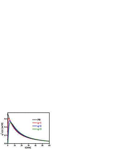
Figure 1: Ion concentration for the counterion-only system for different ion valency $q$. $\varepsilon_{S}=80$ and $\varepsilon_{P}=2.5$. $\sigma=1/(100q)(e/nm^{2})$. The Gouy-Chapman length is kept constant ($l_{GC}=22.7nm$) for counterions of different valencies. The coupling parameter $\Xi$ is $0.031q^{2}$.

The PB theory predicts a universal profile $q^{2}c(z)$ for counterions of different valencies when the Gouy-Chapman length is kept fixed. However, from our scaling analysis in the Introduction, the depletion boundary layer should increase linearly with valency; see Eq. 1. This prediction is borne out by our numerical result as shown in Fig. 1. Therefore, the boundary layer problem becomes more severe for ions of high valency. The scaling of the boundary thickness with the coupling parameter predicted from Eq. 2 is also confirmed by our numerical results (data not shown).

III.2 With Symmetric Salt

When there are added salt ions in the solution, the image force affects the distribution of both the counterions and coions. The PB theory predicts that the double layer structure is characterized by the Debye screening length $\kappa^{-1}$ under the condition that $\kappa^{-1}\ll l_{GC}$, with a monotonically decreasing counterion and monotonically increasing coion distribution. In contrast, both the counterion and coion concentration must vanish at the surface, but their approach to the bulk concentration is different: the coions increases monotonically, while the counterions goes through an overshoot. Furthermore, we find two regimes depending on the relative width of the screening length and the boundary layer thickness, which itself is in turn affected by the screening. At low salt concentration, $\kappa^{-1}\gg d$ and ion depletion is confined in a boundary layer very close to the plate surface; both the ion distribution and electrostatic potential approach the profile predicted by PB beyond the boundary layer. As the salt concentration increases, the width of the depletion boundary layer becomes comparable to the screening length and the two length scales remain comparable thereafter; the image charge interaction then affect the entire range of the double layer. In Figure 2 we show the ion distribution of a $0.1M$ 1:1 electrolyte calculated by our theory. The contrast with the PB result is quite striking.

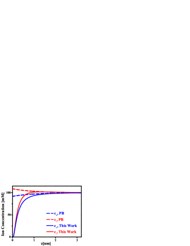
Figure 2: Ion concentration profile for a 1:1 electrolyte solution with $c^{b}=0.1M$. $\varepsilon_{S}=80$, $\varepsilon_{P}=2.5$ and $\sigma=1e/100nm^{2}$.

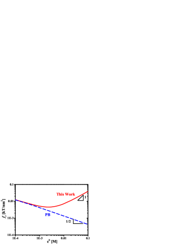
Figure 3: The surface energy $f_{s}$ as a function of the salt concentration for a 1:1 electrolyte solution. $\varepsilon_{S}=80$, $\varepsilon_{P}=2.5$ and $\sigma=1e/100nm^{2}$.

The change in the double layer structure will affect a wealth of interfacial properties. As an example, we show in Figure 3 the surface excess free energy $f_{s}=\int_{0}^{\infty}(w-w^{b})dz$ (where $w$ is the grand free energy density and $w^{b}$ is its bulk value) as a function of the salt concentration. The PB theory predicts a monotonic decrease of $f_{s}$ that scales approximately with $(c^{b})^{-1/2}$, which arises from the electric field contribution in the free energy due to the surface chargeOnuki ; Wang4 . With the inclusion of image charge interaction, our theory shows that $f_{s}$ changes nonmonotonically. At low salt concentration ($c^{b}<10^{-3}M$), $f_{s}$ calculated by our theory follows closely the PB result; this is because the region affected by the image charge repulsion is relatively narrow compared to the screening length, giving a relatively small contribution to the surface excess energy when integrated over the entire solution. As the salt concentration increases ($c^{b}>10^{-2}M$), our theory predicts a sign change in the slope of $f_{s}$ vs. $c^{b}$: $f_{s}$ increases with increasing $c^{b}$, opposite to the PB result. In this concentration regime, the width of the depletion boundary layer is comparable to the Debye screening length, and the entire double layer region is affected by the image charge interaction as shown in Figure 2. The increase in $f_{s}$ is now largely due to the depletion (i.e., negative adsorption) of mobile ions. The slope of $\log(f_{s})$ vs $\log(c^{b})$ is less than $1$ because of the increased screening of the image force as the salt concentration increases. The sign change of $\partial f_{s}/\partial c^{b}$ corresponds to the crossover in the length scale relationship from $\kappa^{-1}\gg d$ to $\kappa^{-1}\approx d$. As the excess surface energy determines the spreading of a liquid drop on a solid surface, this result implies a qualitatively different behavior for the spreading of a drop of electrolyte solution than that predicted by the PB theory. We also note that the nonmonotonic behavior discussed here shares the same physics as the Jones-Ray effectOnuki ; JonesRay ; Bier ; Wang4 for the interfacial tension observed at the water/air and water/oil interfaces.

III.3 With Asymmetric Salt

The effects of image charge become more complex if the salt ions are of unequal valency. Because of the quadratic dependence of the image force on the valency, the higher-valent ions are pushed further away from the surface, necessitating a compensation by the lower-valent ions in the space in between. The difference in the image force between the counterions and the coions induces additional charge separation and hence electric field within the depletion boundary layer. The induced net charge within the boundary layer alters the effective surface charge, which can affect the double layer structure outside the boundary layer. For the case where the coions are of higher valency than the counterions, the induced electric field due to unequal ion depletion counteracts the field generated by the surface charge. With the increase of the salt concentration, the induced field can exceed that generated by the bare surface charge, leading to a sign change in the effective surface charge known as charge inversion. The double layer structure becomes qualitatively different from that predicted by the PB theory as shown in Figure 4: the electrostatic potential is of the opposite sign to the PB result. Excess counterions accumulate in the depletion boundary layer, overcharging the plate surface, while the coions are enriched outside the boundary layer, serving to screen the inverted surface charge. In this case, the PB theory qualitatively fails to describe the entire double layer structure.

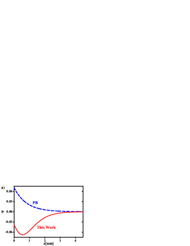
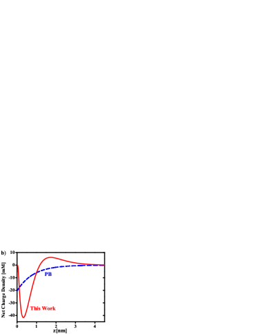
Figure 4: Charge inversion for a 0.05M 2:1 electrolyte solution near a positively charged plate. (a) Dimensionless electrostatic potential and (b) net charge density ($q_{+}c_{+}-q_{-}c_{-}$). $\varepsilon_{S}=80$, $\varepsilon_{P}=2.5$ and $\sigma=1e/100nm^{2}$.

III.4 Uncharged Surface: Image Charge vs. Correlation Effect

The case of an electrolyte solution next to an uncharged surface ($\sigma=0$) reduces to the problem treated by Wagner, Onsager and Samaras. The self energy due to image charge repulsion appears in the Boltzmann factor and is responsible for the depletion layer in the ion distribution near the surface as shown in Figure 5. Note, however, in the original WOS theory as well as in subsequent treatments Monica ; onsager ; Levinsimulation ; Levin1 ; Levin2 , the image charge term was added to the Boltzmann factor ad hoc based on physical intuition, whereas in our theory, its appearance is the result of systematic derivation. Therefore, our theory not only recovers the WOS theory (upon making additional approximations, e.g., by using the constant bulk screening length for the image force potential) but also provides the means for systematically improving the WOS theory. First, our theory captures the anisotropic screening cloud around an ion near the interface due to the spatially varying ion concentration near the surface. The inhomogeneous ionic cloud in the depletion layer and its effect on the screening of the test ion are treated self-consistently in our theory, whereas this inhomogeneous screening is missing in the WOS theory. Second, by including the mean electrostatic potential generated by charge separation, our theory can describe salt solutions with unequal valency such as the case of 2:1 electrolyte shown in Figure 5b. Finally, our theory provides a more accurate expression for the excess free energy by properly accounting for the inhomogeneous screening effect and the fluctuation contribution to the free energy. Thus, we expect our theory to be able to better predict the surface tension of electrolyte solutions in comparison to the WOS theory, especially at higher salt concentrations (where accurate treatment of the screening becomes more important).

The inhomogeneous screening results in a correlation effect that can lead to ion depletion near the surfaceMonica : an ion interacts more favorably with its full ionic atmosphere far away from the surface than in the vicinity of the surface. This correlation effect is stronger for multivalent ions, which pushes them further away from the interface than the monovalent ions. The correlation-induced ion depletion near the surface can take place both with and without the dielectric contrast, and is well captured by our theory, as shown in Figure 5. While the ion depletion without the dielectric contrast is induced by the correlation alone, the ion depletion in the presence of the dielectric contrast is due to both the correlation effect and the image charge effect, which enhance each other. As a result, both ion depletion, as well as charge separation in the case of 2:1 electrolyte, are more pronounced in the presence of image charge than due to correlation alone.

Ion depletion due to correlation alone is most noticeable when the surface is uncharged. When the surface is charged, the surface attraction for the counterions will dominate over such correlation effect in the absence of image charge repulsion. In contrast, depletion due to image charge repulsion persists for both the counterions and coions even when the surface is charged.

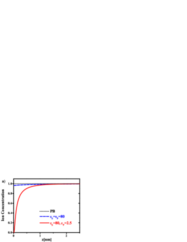
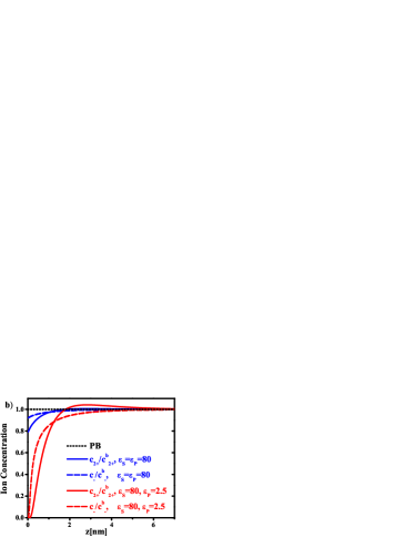
Figure 5: (Color online) Ion concentration (scaled by the bulk ion concentration $c_{\pm}^{b}$) for (a) 0.01M 1:1 electrolyte solution ($c_{+}=c_{-}$) and (b) 0.01M 2:1 electrolyte solution near an uncharged interface ($\sigma=0$) with dielectric contrast ($\varepsilon_{S}=80$, $\varepsilon_{P}=2.5$) in comparison with the case without dielectric contrast ($\varepsilon_{S}=\varepsilon_{P}=80$). Profiles calculated by our theory are shown by colored lines; results from the PB theory are given as black dot lines.

IV Conclusions

In this work, we have shown that the image charge repulsion creates a depletion boundary layer near a dielectric surface, which cannot be captured by a regular perturbation method. Using a nonperturbative approach based on a variational functional formulation, we find that the self energy of the ion, which includes contributions from both the image charge interaction and the interionic correlation, appears explicitly in the Boltzmann factor for the ion distribution, resulting in a self-energy modified Poisson-Boltzmann equation as the appropriate theory for describing the physical weak-coupling condition. This image-charge self energy is not diminished by reducing the surface or the ionic strength in the solution; in the presence of a significant dielectric discontinuity, there is no limiting condition for which the PB theory is valid. For zero surface charge, our theory reduces to the WOS theory upon further approximations. Thus, our theory provides both the justification for the WOS theory and means for systematically improving the WOS theory, for example, by including the mean electrostatic potential generated by the charge separation in salt solutions with unequal valency or other asymmetries between the cation and anions, such as different size and polarizabilityLevin1 .

The weak-coupling condition in the presence of dielectric discontinuity covers many soft-matter and biophysical systems. Many phenomena, such as the surface tension of electrolyte solutionsSurfacetension1 ; Surfacetension2 , salt effects on bubble coalescenceBubble , and the ion conductivity in artificial and biological ion-channelsChannel1 ; Channel2 ; Channel3 , cannot be explained, even qualitatively, by the PB theory. The presence of the image charge interaction results in a very different picture of the electrical double layer from that provided by the PB theory, and can give rise to such phenomena as like-charge attraction and charge inversion even in the weak-coupling conditionWang3 ; these phenomena have usually been associated with the strong-coupling condition. The PB theory has played a foundational role in colloidal and interfacial sciences: the DLVO theory, interpretation of the zeta potential, experimental determination of the surface charge and the Hamaker constant, are all based on the PB theoryIsraelachvili . With the inclusion of the image charge interaction, some of the well known and accepted results will have to be reexamined.

Appendix A Derivation of the key equations in Section II.A

We define $\chi\equiv\phi+i\psi$ as the fluctuation part of the field $\phi$, which is a Gaussian variable by our ansatz. The variational grand free energy can be approximated by the r.h.s of Eq. 10 as

$$W =-\ln\Omega_{ref}+\langle L\left[\phi\right]-L_{ref}\left[\phi\right]\rangle=-\frac{1}{2}\ln\left(\frac{\det{\bf G}}{\det{\bf G}_{0}}\right)$$ (24)

$$- \frac{1}{2}\int d{\bf r}d{\bf r}^{\prime}\{\delta({\bf r}^{\prime}-{\bf r})\left[\epsilon(\nabla\psi)^{2}-\epsilon\langle(\nabla\chi)^{2}\rangle\right]+G^{-1}({\bf r},{\bf r}^{\prime})$$

$$\times \langle\chi({\bf r})\chi({\bf r}^{\prime})\rangle\}+\int d{\bf r}[\rho_{ex}\psi-\Gamma\lambda_{+}{\rm e}^{-q_{+}\psi}\langle{\rm e}^{-i{\hat{h}}_{+}\chi}\rangle$$

$$+ \Gamma\lambda_{-}{\rm e}^{q_{-}\psi}\langle{\rm e}^{i{\hat{h}}_{-}\chi}\rangle]$$

The averages in Eq. 24 can be evaluated exactly because the distribution of $\chi$ is Gaussian. Noting that

$$\langle\chi({\bf r})\chi({\bf r}^{\prime})\rangle=G({\bf r},{\bf r}^{\prime})$$ (25)

we have

$$\int d{\bf r}d{\bf r}^{\prime}\delta({\bf r}-{\bf r}^{\prime})\epsilon\langle(\nabla\chi)^{2}\rangle$$

$$=\int d{\bf r}d{\bf r}^{\prime}\nabla_{\bf r}\cdot\left[\epsilon({\bf r})\nabla_{\bf r}^{\prime}\delta({\bf r}-{\bf r}^{\prime})\right]G({\bf r},{\bf r}^{\prime})$$ (26)

and

$$\langle{\rm e}^{\mp i{\hat{h}}_{\pm}\chi}\rangle=\exp[ - \frac{1}{2}\int d{\bf r}^{\prime}d{\bf r}^{\prime\prime}h_{\pm}({\bf r}-{\bf r}^{\prime})G({\bf r}^{\prime},{\bf r}^{\prime\prime})$$ (27)

$$\times h_{\pm}({\bf r}^{\prime\prime}-{\bf r})]$$

Substituting Eqs. 25-27 into Eq. 24, we obtain the variational form of the grand free energy as

$$W =-\frac{1}{2}\ln\left(\frac{\det{\bf G}}{\det{\bf G}_{0}}\right)-\frac{1}{2}\int d{\bf r}\epsilon(\nabla\psi)^{2}$$ (28)

$$- \frac{1}{2}\int d{\bf r}d{\bf r}^{\prime}\left[G^{-1}({\bf r},{\bf r}^{\prime})-G_{0}^{-1}({\bf r},{\bf r}^{\prime})\right]G({\bf r},{\bf r}^{\prime})$$

$$+ \int d{\bf r}\left(\rho_{ex}\psi-\Gamma\lambda_{+}{\rm e}^{-q_{+}\psi-u_{+}}-\Gamma\lambda_{-}{\rm e}^{q_{-}\psi-u_{-}}\right)$$

where $u_{\pm}$ is the self energy of the ions given by Eq. 15. Minimizing Eq. 28 with respect to $\psi$ and $G$ gives rise to Eq. 13 and Eq. 14 in the main text.

Appendix B Simplification of the fluctuation contribution in the free energy

Making use of Eq. 13 and Eq. 14, Eq. 28 can be simplified as

$$W = -\int d{\bf r}\left[c_{+}({\bf r})+c_{-}({\bf r})\right]$$ (29)

$$+ \frac{1}{2}\int d{\bf r}\psi({\bf r})\left[\rho_{ex}({\bf r})-q_{+}c_{+}({\bf r})+q_{-}c_{-}({\bf r})\right]$$

$$- \frac{1}{2}\ln\left(\frac{\det{\bf G}}{\det{\bf G}_{0}}\right)-\int d{\bf r}I({\bf r})G({\bf r},{\bf r})$$

The last two terms in Eq. 29 are due to the fluctuation contribution. We note that the Green function equation (Eq. 14) can be written in the matrix form as

$${\bf G}_{0}^{-1}{\bf G}+2I({\bf r}){\bf G}={\bf I}$$ (30)

where ${\bf I}$ is the identity matrix (not to be confused with the local ionic strength $I$). Right multiplication of the above equation by ${\bf G}^{-1}$, we obtain

$${\bf G}^{-1}={\bf G}_{0}^{-1}+2I({\bf r}){\bf I}$$ (31)

Note also that

$$\ln\left(\frac{\det{\bf G}}{\det{\bf G}}_{0}\right)=\ln\det{\bf G}-\ln\det{\bf G}_{0}$$

$$=\int d{\bf r}\int d{\bf r}^{\prime}\int_{G_{0}^{-1}}^{G^{-1}}\frac{\delta\ln\det{\bf G}}{\delta G^{-1}({\bf r},{\bf r}^{\prime})}\delta G^{-1}({\bf r},{\bf r}^{\prime})$$ (32)

The innermost integral is a functional integration over $G^{-1}$ from $G_{0}^{-1}$ to $G^{-1}$. Since $\ln\det{\bf G}$ is the result of a Gaussian functional integral, we have

$$\frac{\delta\ln\det{\bf G}}{\delta G^{-1}({\bf r},{\bf r}^{\prime})}=-G({\bf r},{\bf r}^{\prime})$$ (33)

Therefore,

$$\ln\left(\frac{\det{\bf G}}{\det{\bf G}_{0}}\right)=-\int d{\bf r}\int d{\bf r}^{\prime}\int_{G_{0}^{-1}}^{G^{-1}}G({\bf r},{\bf r}^{\prime})\delta G^{-1}({\bf r},{\bf r}^{\prime})$$ (34)

As the integration goes from $G_{0}^{-1}$ to $G^{-1}$, the integrand changes from $G_{0}$ to $G$. From Eq. 31, a convenient path for integrating Eq. 34 is to introduce a continuous “charging” variable $\eta$ that goes from 0 to 1 multiplying the $2I$ term in Eq. 31, while keeping the density profile fixed. Obviously the Green function is $G_{0}$ for $\eta=0$ and is $G$ for $\eta=1$. For any intermediate value, we denote the Green function as $G({\bf r},{\bf r}^{\prime};\eta)$. Using Eq. 31, the above integral becomes,

$$\ln \left(\frac{\det{\bf G}}{\det{\bf G}_{0}}\right)=-2\int d{\bf r}\int d{\bf r}^{\prime}\int_{0}^{1}I({\bf r})\delta({\bf r}-{\bf r}^{\prime})$$ (35)

$$\times G({\bf r},{\bf r}^{\prime};\eta)d\eta=-2\int d{\bf r}I({\bf r})\int_{0}^{1}G({\bf r},{\bf r};\eta)d\eta$$

where $G({\bf r},{\bf r};\eta)$ is to be understood as the limit $G({\bf r},{\bf r};\eta)=\lim_{{\bf r}^{\prime}\rightarrow{\bf r}}G({\bf r},{\bf r}^{\prime};\eta)$, and the Green function $G({\bf r},{\bf r}^{\prime};\eta)$ is the solution of

$$-\nabla\cdot\left[\epsilon\nabla G({\bf r},{\bf r}^{\prime})\right]+2\eta I({\bf r})G({\bf r},{\bf r}^{\prime})=\delta({\bf r}-{\bf r}^{\prime})$$ (36)

With Eq. 35, the fluctuation contribution to the free energy is

$$\frac{1}{2}\ln\left(\frac{\det{\bf G}}{\det{\bf G}_{0}}\right)+\int d{\bf r}I({\bf r})G({\bf r},{\bf r})$$

$$=-\int d{\bf r}I({\bf r})\int_{0}^{1}d\eta\left[G({\bf r},{\bf r};\eta)-G({\bf r},{\bf r})\right]$$ (37)

which is finite even in the point-charge limit.

References

- (1) J. N. Israelachvili, Intermolecular and surface forces, 2nd Ed. (Academic, London, 1992).
- (2) W. M. Gelbart, R. F. Bruinsma, P. A. Pincus and V. A. Parsegian, Phys. Today, 53, 38-44 (2000).
- (3) Y. Levin, Rep. Prog. Phys., 65, 1577-1632, (2002).
- (4) B. Honig and A. Nicholls, Science, 268, 1144-1149 (1995).
- (5) G. M. Luo, S. Malkova, J. Yoon, D. G. Schultz, B. H. Lin, M. Meron, I. Benjamin, P. Vanysek and M. L. Schlossman, Science, 311, 216-218 (2006).
- (6) R. Kjellander, S. Marcelja, R. M. Pashley and J. P. A. Quirk, J. Chem. Phys., 92, 4399-4407 (1990).
- (7) W. R. Bowen and A. Q. Sharif, Nature, 393, 663-665 (1998).
- (8) Y. S. Jho, M. Kandu, A. Naji, R. Podgornik, M. W. Kim and P. A. Pincus, Phys. Rev. Lett., 101, 188101 (2008).
- (9) P. Kekicheff, S. Marcelja, T. J. Senden and V. E. Shubin, J. Chem. Phys., 99, 6098-6113 (1993).
- (10) T. T. Nguyen, A. Y. Grosberg and B. I. Shklovskii, Phys. Rev. Lett., 85, 1568-1571 (2000).
- (11) A. Y. Grosberg, T. T. Nguyen and B. I. Shklovskii, Rev. Mod. Phys., 74, 329-345 (2002).
- (12) K. Besteman, M. A. G. Zevenbergen, H. A. Heering and S. G. Lemay, Phys. Rev. Lett., 93, 170802 (2004).
- (13) R. Kjellander, T. Akesson, B. Jonsson and S. Marcelja, J. Chem. Phys., 97, 1424-1431 (1992).
- (14) J. W. Zwanikken and M. Olvera de la Cruz, Proc. Natl. Acad. Sci. USA, 110, 5301-5308 (2013).
- (15) A. Naji, S. Jungblut, A. G. Moreira and R. R. Netz, Physica A, 352, 131-170 (2005).
- (16) J. C. Neu, Phys. Rev. Lett., 82, 1072-1074 (1999).
- (17) P. Attard, D. J. Mitchell and B. W. Ninham, J. Chem. Phys., 88, 4987-4996 (1988).
- (18) P. Attard, D. J. Mitchell and B. W. Ninham, J. Chem. Phys., 89, 4358-4367 (1988).
- (19) R. R. Netz and H. Orland, Eur. Phys. J. E, 1, 203-214 (2000).
- (20) R. R. Netz, Eur. Phys. J. E, 5, 557-574 (2001).
- (21) M. Kandu and R. Podgornik, Eur. Phys. J. E, 23, 265-274 (2007).
- (22) R. Podgornik and B. Zeks, J. Chem. Soc., 84, 611 (1989).
- (23) R. Podgornik, J. Chem. Phys., 91, 5840-5849 (1989).
- (24) A. Naji, M. Kandu, J. Forsman and R. Podgornik, J. Chem. Phys., 139, 150901 (2013).
- (25) C. Wagner, Phys. Z. 25, 474-477 (1924).
- (26) L. Onsager and N. N. T. Samaras, J. Chem. Phys., 2, 528-536 (1933).
- (27) A. Bakhshandeh, A. P. dos Santos and Y. Levin, Phys. Rev. Lett., 107, 107801 (2011).
- (28) R. Kjellander and S. Marcelja, Chem. Phys. Lett., 112, 49-53 (1984).
- (29) R.R. Netz and H. Orland, Eur. Phys. J. E,11, 301-311, (2003).
- (30) Z. -G. Wang, Phys. Rev. E, 81, 021501 (2010).
- (31) D. S. Dean and R. R. Horgan, Phys. Rev. E, 69, 061603 (2002).
- (32) S. L. Carnie and G. M. Torrie, Adv. Chem. Phys., 56, 141-253 (1984).
- (33) F. P. Buff and F. H. Stillinger, J. Chem. Phys., 39, 1911-1923 (1963).
- (34) G. M. Bell and S. Levine, J. Chem. Phys., 49, 4584-4599 (1968).
- (35) Y. Levin and J. E. Flores-Mena, Europhys. Lett. 56, 187-192 (2001).
- (36) Y. Levin, A. P. dos Santos and A. Diehl, Phys. Rev. Lett. 103, 257802 (2009).
- (37) Z. L. Xu, M. M. Ma and P. Liu, Phys. Rev. E, 90, 013307 (2014).
- (38) Eq. 22 is solved with 2000 grid points along the axis for each . The Dirac delta function is approximated by the Kronecker delta. Numerical integration in the space (Eq. 20) is performed using the Simpson method with 200 grid points.
- (39) A. Onuki, J. Chem. Phys. 128, 224704 (2008);
- (40) R. Wang and Z.-G. Wang, J. Chem. Phys. 135, 014707 (2011).
- (41) G. Jones and W. A. Ray, J. Am. Chem. Soc. 59, 187-198 (1937).
- (42) M. Bier, J. Zwanikken and R.van Roij, Phys. Rev. Lett. 101, 046104 (2008).
- (43) W. Kunz, P. Lo Nostro, and B.W. Ninham, Curr. Opin. Colloid Interf. Sci. 9, 1-18 (2004).
- (44) B. C. Garrett, Science 303, 1146-1147 (2004).
- (45) V. S. J. Craig, B. W. Ninham and R. M. Pashley, Nature 364, 317-319 (1993).
- (46) A. Parsegian, Nature, 221, 844-846 (1969).
- (47) T. Bastug and S. Kuyucak, Biophys. J., 84, 2871-2882 (2003).
- (48) S. Buyukdagli, M. Manghi and J. Palmeri, Phys. Rev, Lett., 105, 158103, (2010).
- (49) R. Wang and Z. -G. Wang, J. Chem. Phys., 139, 124702, (2013).