Limits on Polarized Leakage for the PAPER Epoch of Reionization Measurements at 126 and 164 MHz

Abstract

Polarized foreground emission is a potential contaminant of attempts to measure the fluctuation power spectrum of highly redshifted 21 cm Hi emission from the Epoch of Reionization. Using the Donald C. Backer Precision Array for Probing the Epoch of Reionization, we present limits on the observed power spectra of all four Stokes parameters in two frequency bands, centered at 126 MHz ($z=10.3$) and 164 MHz ($z=7.66$), for a three-month observing campaign of a deployment involving 32 antennas, for which unpolarized power spectrum results have been reported at $z=7.7$ (Parsons et al., 2014) and at $7.5<z<10.5$ (Jacobs et al., 2015). The power spectra in this paper are processed in the same way as in those works, and show no definitive detection of polarized power. This nondetection is consistent with what is known about polarized sources, combined with the suppression of polarized power by fluctuations in the ionospheric rotation measure, which can strongly affect Stokes $Q$ and $U$. We are able to show that the net effect of polarized leakage is a negligible contribution at the levels of the limits reported by Parsons et al. (2014) and Jacobs et al. (2015).

1. Introduction

Polarized emission at meter wavelengths is a potentially problematic foreground for experiments seeking to measure the 21 cm power spectrum of the Epoch of Reionization (EoR). Smooth-spectrum sources occupy a well-defined “wedge” in the cylindrical $(k_{\parallel},k_{\perp})$ space of the EoR power spectrum (e.g., Morales et al., 2012; Pober et al., 2013), but it has been understood for some time (e.g., Geil et al., 2011; Pen et al., 2009) that Faraday-rotated polarized emission can contaminate the measurement of unpolarized EoR emission. When mapped into the power spectrum, this Faraday-rotated polarized emission generates power that mimics the high $k_{\parallel}$ emission of the EoR, scattering power into the otherwise clean EoR window. Moore et al. (2013, hereafter M13) simulated the effects of the low-level forest of weak, polarized point sources leaking into the full 3D EoR power spectrum. M13 used the best measurements available at the time, notably the existing (unpolarized) point source surveys (Hales et al., 1988; Cohen et al., 2004) and the few polarization measurements below 200 MHz (Pen et al., 2009; Bernardi et al., 2009), and found that the level of emission could be problematic for any experiment with $\sim 1\%$ leakage from Stokes $Q\to I$. More recent work, discussed further below, suggests that the actual level of point source polarization is lower than M13 assumed (Asad et al., 2015). It may also be possible to address polarization leakage due to wide-field beams with modest calibration requirements, as demonstrated with the Murchison Widefield Array (MWA, a precursor of SKA, the Square Kilometer Array) (Sutinjo et al., 2015a) and ongoing characterization of the SKA prototype antennas (Sutinjo et al., 2015b).

Polarized emission may arise from diffuse (presumably Galactic) emission and point sources. Historically, the first measurements of the polarization of diffuse emission in the Southern Hemisphere at frequencies below 1.4 GHz were reported by Mathewson & Milne (1964, 1965), who used the Parkes telescope at 408 MHz and 0.8° resolution to follow on the previous work of Westerhout et al. (1962). Spoelstra (1984) provided a summary of the situation at frequencies between 408 and 1411 MHz, noting the low rotation measures of this emission ($<8~{}\rm{rad~{}m^{-2}}$) with a polarization fraction of $\sim 35\%$ near 1.4 GHz and notable depolarization at lower frequencies. The emission seems to be largely due to nearby sources ($\sim$450 pc), and fluctuates on scales from 1 - 10°. More recent analysis of the angular power spectrum of diffuse, polarized fluctuations by La Porta & Burigana (2006) suggests that the fluctuations continue to smaller scales as a power law, depending on frequency. Bernardi et al. (2013, hereafter B13), who conducted a 2400 square degree survey using the MWA at 189 MHz, and Jelić et al. (2014, hereafter Je14), both reported significant amounts of weakly polarized emission on angular scales between a few degrees for B13 and a few tens of arcminutes for Je14. The rotation measure (RM) $|\Phi|\leq 25~{}\rm{rad~{}m}^{-2}$ in all cases.

Regarding point sources, the number of bright sources below 200 MHz reported in the literature is small (although it should also be pointed out that only small parts of the southern and northern sky have been surveyed for such sources). Of particular interest in determining the polarization contamination is the linearly polarized fraction $p=\sqrt{(Q^{2}+U^{2})/I^{2}}$ of sources (where $I$, $Q$, and $U$ are the Stokes parameters), and, in the absence of low-frequency measurements, how this scales from higher frequencies. B13 detected one polarized point source at 189 MHz, PMN J0351-2744, with a polarization fraction $p=0.02$ and polarized flux of 320 mJy. At somewhat higher frequencies (350 MHz), Gießübel et al. (2013) studied sources behind M31 and found that $p_{\rm 350~{}MHz}=0.14~{}p_{\rm 1.4~{}GHz}$, with typical values of a few percent at 350 MHz. A study of the depolarization of point sources by Farnes et al. (2014) showed a systematic trend for depolarization of steep-spectrum point sources as frequency decreased, resulting in very low polarization fractions ($p\ll 0.01$) below 300 MHz. In a measurement of M51 using LOFAR between 115 and 175 MHz, Mulcahy et al. (2014) detected 6 background sources with Stokes $I$ between 44 and 1500 mJy. They detect two “sources” with relatively large polarized fractions (0.026 and 0.029), but these are the lobes of radio galaxies with unpolarized cores. If one were to include the flux from the core, thus giving the total polarized fraction integrated over the galaxy, this would be lower. For the unresolved sources, the polarized fractions are all $<2.8\times 10^{-3}$. Depolarization from 1.4 GHz ranged between 0.03 and 0.2 for the six sources. Importantly, Mulcahy et al. (2014) had very high angular resolution (20-25″) relative to B13 and the Donald C. Backer Precision Array for Probing the Epoch of Reionization (PAPER), thus minimizing beam depolarization effects from integrating over sources.

It is worth noting that the reported rotation measures for point sources vary over the range of values reported in the all-sky RM map of Oppermann et al. (2012), whereas the diffuse emission typically shows low RM. This is consistent with the interpretation of this emission as nearby diffuse Galactic synchrotron. As discussed in Jelić et al. (2010), polarized synchrotron generated from within a magnetized, ionized plasma will be depolarized, and will further show structure in the RM spectrum of the source. The result is a lower apparent Faraday depth. By contrast, extragalactic point sources see a large Faraday column through the Galaxy, resulting in a high Faraday depth.

The goal of this paper is to determine, from measured polarization power spectra, the extent of possible polarized leakage on the upper limits on the EoR power spectrum previously reported from PAPER in Parsons et al. (2014, hereafter P14) and Jacobs et al. (2015, hereafter J15). We begin in Section 2 by reviewing key points of the effect of polarization on the EoR power spectrum. We describe the dataset and processing steps in Section 3, and present power spectra from two frequency bands in all four Stokes parameters in Section 4 along with implications of these measurements for the level of polarized leakage into the 21 cm EoR power spectrum. We conclude in Section 5.

2. The Problem of Polarization

In this section, we will briefly review the problem of polarization for EoR power spectrum measurements. We recall that the index of refraction of an ionized, magnetized plasma is birefringent. The left- and right-circular polarizations of an electromagnetic wave passing through such a plasma undergo different phase shifts, known as Faraday rotation, such that the phase difference $\Delta\varphi$ of the light becomes

$$\Delta\varphi=\frac{e^{2}}{(m_{e}c^{2})^{2}}\lambda^{2}\int n_{e}(s)B_{\parallel}(s)\mathrm{d}s\equiv\lambda^{2}\Phi,$$ (1)

where $n_{e}$ is the electron density of the plasma, $B_{\parallel}$ is the component of the magnetic field along the line of sight, $e$ and $m_{e}$ are the electron charge and mass, $\lambda^{2}$ is the wavelength of the incident light, and the integral extends along the line of sight. Equation 1 defines the rotation measure $\Phi$. Faraday rotation affects the linear components of the Stokes parameters such that a polarized source with intrinsic Stokes $Q$ and $U$, when viewed through a magnetized plasma, will have measured Stokes parameters

$$(Q+iU)_{meas}=e^{-2i\lambda^{2}\Phi}(Q+iU)_{intr}$$ (2)

The frequency structure induced by Faraday rotation differs from normal smooth-spectrum foregrounds, and exhibits high covariance with the high line-of-sight $k_{\parallel}$ modes, which are typically free of synchrotron foreground emission (e.g. Morales et al., 2006, 2012; Parsons et al., 2012b). In fact, there is a nearly one-to-one correspondence between a $\Phi$ mode and the $k_{\parallel}$ mode it most infects, given by

$$k_{\parallel}=4\frac{H(z)}{c(1+z)}\Phi\lambda^{2},$$ (3)

where $z$ is the redshift of the observation, $H(z)$ is the Hubble parameter at that redshift, $\lambda$ is the wavelength of the observation, and $\Phi$ is the rotation measure in question. At 164 MHz, the central frequency of one of the bands we present, a typical rotation measure of $20\ {\rm{rad~{}m}^{-2}}$ will infect $k_{\parallel}$ values of around $0.25\ h\,{\rm Mpc^{-1}}$, well outside the horizon limit for smooth-spectrum foregrounds on short baselines ($k\approx 0.05\ h\,\mathrm{Mpc}^{-1}$ for $z=7.7$ and a 30 m baseline).

The power spectrum for 21cm EoR measurements is unpolarized, so the frequency structure induced by Faraday rotation must leak into $I$ measurements through instrumental effects. We note that any instrumental effect that leaks Stokes $Q$ or $U$ into $I$ is subject to the kind of contamination we discuss here. For PAPER, the particular form of the dominant leakage comes about as follows. Since PAPER has little imaging capability in its maximum-redundancy configuration, we cannot form Stokes parameters in the image plane, but rather, we combine visibilities as if they were images, by defining

$$\begin{pmatrix}V_{I}\\ V_{Q}\\ V_{U}\\ V_{V}\end{pmatrix}=\frac{1}{2}\begin{pmatrix}1&0&0&1\\ 1&0&0&-1\\ 0&1&1&0\\ 0&-i&i&0\end{pmatrix}\begin{pmatrix}V_{xx}\\ V_{xy}\\ V_{yx}\\ V_{yy}\end{pmatrix},$$ (4)

where $V_{xx}$, etc., are the linearly polarized, measured visibilities for each frequency and time, and $V_{I}$, etc., are the “Stokes visibilities”. The detailed expression for the leakage of Stokes $Q$, $U$, and $V$ into $I$ due to wide-field beams has been explored elsewhere (e.g., Shaw et al., 2015), and we defer a detailed study of this effect for PAPER to future work. Considerable simplification occurs in the limit that the two feeds produce orthogonal responses to the two electric field polarizations everywhere on the sphere, which is not strictly achievable in practice (see, e.g., Carozzi & Woan, 2009), but is a good approximation over most of the 45° FWHM PAPER field of view. In this limit, expanding the first row of the matrix and expressing the visibilities in terms of the beams $A_{p}$ for polarization $p$, the baseline $\mathbf{b}$, the unit vector $\hat{s}$, and the intrinsic polarized signals $I$ and $Q$, we find

$$V_{I}=\int(A_{xx}+A_{yy})Ie^{-2\pi i\mathbf{b}\cdot\hat{s}\nu/c}\ \mathrm{d}\Omega$$

$$+\int(A_{xx}-A_{yy})Qe^{-2\pi i\mathbf{b}\cdot\hat{s}\nu/c}\ \mathrm{d}\Omega.$$ (5)

The expression for $V_{Q}$ is similar, with $I$ and $Q$ interchanged. Thus, if the primary beam of each element is not symmetric under rotations of 90^∘, then the $I$ visibility will have a contribution from both $I$ and $Q$. This provides the mechanism for the spectrally non-smooth Faraday-rotated polarized emission to infect the typically unpolarized 21cm EoR power spectrum for PAPER.

3. Data Processing

The data used to create these results are nearly identical to those presented in this paper’s sister papers, P14 and J15. We will review the processing steps presented there, highlighting slight modifications.

PAPER’s 32 antennas were arranged into a 4 row $\times$ 8 column grid during the 2011-2012 season (PSA32), when these data were taken. The east-west row spacing was 30 m, and the north-south column spacing was 4 m. This choice of antenna configuration maximizes baseline redundancy, achieving heightened sensitivity (Parsons et al., 2012a), and allows for the redundant calibration of visibilities (e.g. Liu et al., 2010).

This data set consists of data taken continuously from Julian date 2455903 until 2455985, for a total of 82 days of observation. The effective integration time for any point on the sky is shown in Figure 1. Data are not considered when the sun is above -5^∘ in altitude.

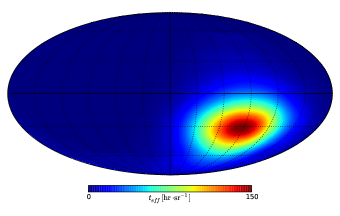
Figure 1.— Effective integration time per pointing, as a function of position on the sphere. This metric is defined to give the total integration time when integrated over position on the sphere. The total field of view surveyed is 2.39 sr. RA zero is at the center of the Mollweide projection, and increases to the right, wrapping around the sphere. The maximum occurs in RA at approximately 6h, and in Dec at approximately -30°, above the latitude of the array.

	Center frequency	Total bandwidth	Channel width	Redshift	Collecting area	System temperature	Beam Leakage Ratio
	$\nu_{c}$ [MHz]	$\Delta\nu$ [MHz]	$\delta\nu$ [kHz]	$z$	$A_{\rm eff}$ [m2]	$T_{\rm sys}$ [K]	$\mathcal{A}_{-}/\mathcal{A}_{+}$ (Eq. 19)
Band I	126	7.9	493	10.3	4.47	836	$3.3\times 10^{-3}$
Band II	164	9.4	493	7.66	5.80	505	$2.2\times 10^{-3}$

Table 1 Observational Parameters

3.1. Initial Processing

We begin with an excision of radio-frequency interference (RFI), a three-step process. First, we flag known frequency channels containing nearly constant RFI, for example, the 137 MHz frequency bin that contains the continuous signal from a constellation of communications satellites. Away from these regions, the fraction of data flagged is $\ll 1\%$ of the total. Next, we subtract adjacent time and frequency channels from each other to cancel the bulk of the signal, and flag $6\sigma$ outliers in the differenced data. Finally, we remove a foreground model and flag $4\sigma$ outliers in the residual spectra.

Once RFI excision has taken place, we low-pass filter and decimate the data in time and frequency, in the manner described in Appendix A of P14. This reduces the data volume by roughly a factor of forty — from 1024 to 203 channels, and from integration times of 10 seconds to 34 seconds — and preserves all celestial signal, including the EoR.

Next, we derive a fiducial calibration solution for a single day’s worth of data. We begin by solving for antenna-based gains and electrical delays which enforce redundant measurements across redundant baselines in the array. This reduces the calibration solutions to a single, overall gain and delay per polarization of the array, which we solve by fitting visibilities to a model of Pictor A, correcting for the primary beam gain towards Pictor A, as in Jacobs et al. (2013). For sources at zenith, calibration errors are a few percent. We apply this fiducial calibration solution to all data.

We develop a model of the smooth-spectrum foregrounds for each integration and each baseline by constructing a spectrum of delay components over the full available bandwidth (100-200 MHz) using a 1D CLEAN algorithm. We constraint these CLEAN components to lie within the entire horizon-to-horizon range with an additional extent of 15 ns beyond either horizon. This procedure does not affect high-delay signal due to the EoR, but both removes foreground signal and deconvolves by an uneven RFI flagging kernel. We subtract this model from the data at each integration and baseline. This procedure is described in P14 and J15.

Finally, we remove cross-talk, defined as an offset in visibilities constant with time. For each baseline, and for each day, we subtract the nightly average of the data, enforcing mean zero visibilities.

3.2. Polarization Calibration

To begin a discussion of polarization calibration, we summarize the redundant calibration procedure we take. First, we take the set of $xx$ and $yy$ visibilities and treat them like independent arrays. Within each of these arrays, we solve for the $N_{\rm ant}$ antenna-based gains and $N_{\rm ant}$ antenna-based electrical delays which force all baselines of a certain type to be redundant with a fiducial baseline in each type. This leaves three calibration terms per polarization to be solved for: an overall flux scale, and two delays that set the three baseline types to the same phase reference. We solve for these three by fitting the redundant visibilities to a model of Pictor A (Jacobs et al., 2013).

So far, we have made the reasonable assumption that $I$ dominates the $xx$ and $yy$ visibilities. If we also assume that the gains and delays are truly antenna-based, then we can apply the calibration solutions from those visibilities to the $xy$ and $yx$ visibilities. This procedure omits one more calibration term, which sets the $x$ and $y$ solutions to the same reference phase: the delay between the $x$ and $y$ solutions, $\tau_{xy}$.

To solve for this delay, we minimize the quantity

$$\chi^{2}=\sum_{i,j}\left|V_{ij}^{xy}-V_{ij}^{yx}\exp\{-2\pi i\tau_{xy}\nu\}\right|^{2},$$ (6)

where the sum runs over antenna pairs $i,j$, finding the electrical delay that minimizes $V_{V}$ in the least-squares sense. This potentially nulls some signal in $V_{V}$, but we do not expect any significant signal in $V$ at these frequencies. This method of polarization calibration is similar to that presented in Cotton (2012), but rather than maximizing $V_{U}$, we are minimizing $V_{V}$. By assuming that gains are antenna-based and that the flux in $V_{xx}$ and $V_{yy}$ is dominated by unpolarized emission, we need not correct for gain differences between $V_{xy}$ and $V_{yx}$ (the relevant gains having already come from the $xx$ and $yy$ solutions).

3.3. Averaging Multiple Days

As a final excision of spurious signals (most likely due to RFI), on each day, we flag outlying measurements in each bin of local sidereal time (LST). We use the measurement of $T_{\rm sys}$ outlined in Section 3.5 to estimate the variance of each bin, and flag $3\sigma$ outliers.

If the data followed a normal distribution, consistent with pure, thermal noise, then this procedure would flag around one measurement in each frequency/LST bin, causing a slight miscalculation of statistics post-flagging. To counteract this effect, we calculate the ratio of the variance of a normal distribution, truncated at $\pm 3\sigma$ (97.3%). We increase all errors in the power spectrum by a factor of $1.03\approx 1/97.3\%$ to account for this effect.

We compute the mean of the RFI-removed data for each bin of LST and frequency, creating a data set that consists of the average over all observations for each LST bin, literally an average day. We continue analysis on these data.

3.4. Final Processing

After visibilities are averaged in LST, a final round of cross-talk removal is performed. Again, we simply subtract the time average across LST from the data.

In the penultimate processing step, we pass the data through a low-pass filter in time. Parsons & Backer (2009) and Appendix A of P14 describe the celestial limits of the fringe rate $f$ for drift-scan arrays as $b_{E}\omega_{\oplus}\cos\lambda\leq f\leq b_{E}\omega_{\oplus}$, where $b_{E}$ is the east-west component of the baseline, $\omega_{\oplus}$ is the angular velocity of the Earth’s rotation, and $\lambda$ is the latitude of the observation. We filter the data in time using a boxcar filter in fringe-rate space, defined as one on $0\leq f\leq b_{E}\omega_{\oplus}$ and zero elsewhere. While this does null some celestial emission (roughly the area between the south celestial pole and the southern horizon), its effect is small, since the primary beam heavily attenuates these areas of the sky. We null these fringe rates as an additional step of cross-talk removal.

Finally, we combine the linearly polarized visibilities into Stokes visibilities, as in Equation 4.

3.5. System Temperature

Once initial preprocessing has been completed, we take advantage of nightly redundancy as a final check on the data. Since PAPER is a transit array, measurements taken at the same LST on different nights should be totally redundant. This redundancy allows us to measure the system temperature via fluctuations in signal in the same LST bin from day to day.

First, we compute the variance in each frequency and LST bin over all nights of data $\sigma_{Jy}^{2}(\nu,t)$, and convert this variance into a measure of the system temperature $T_{\rm sys}$. This measurement is totally independent of the following power spectral analysis, and can be used to quantify the level of systematic and statistical uncertainty in the power spectra. It complements measurements of $T_{\rm sys}$ from the uncertainties in power spectra in P14 and J15. The variance computed in each frequency/LST bin $\sigma_{Jy}^{2}(\nu,t)$ is converted into a system temperature in the usual fashion:

$$T_{\rm sys}(\nu,t)=\frac{A_{\rm eff}}{k_{B}}\frac{\sigma_{Jy}}{\sqrt{2\delta\nu t_{\rm int}}},$$ (7)

where $A_{\rm eff}$ is the effective area of the antenna, $k_{B}$ is the Boltzmann constant, $\delta\nu$ is the channel width, and $t_{\rm int}$ is the effective integration time of the LST bin.

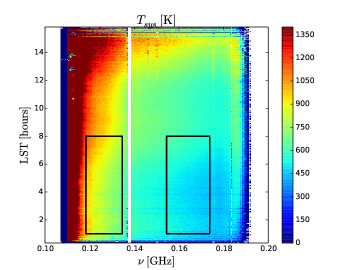
Figure 2.— System temperature in Kelvin as a function of local sidereal time (LST) and frequency $\nu$, calculated by Equation 7. Solid black boxes enclose the area used to compute the power spectrum. The persistent RFI mentioned in Section 3.1, as well as the band edges, appear white in this figure.

Figure 2 shows the measured system temperature for each frequency and LST bin collected during the PSA32 observing season. To further summarize our data’s variance, we average $T_{\rm sys}(\nu,t)$ over the time axis and frequency axis. The frequency-averaged system temperature at center frequency $\nu_{c}$ may be computed as

$$\langle T_{sys}\rangle_{\nu_{c}}(t)\equiv\frac{\int_{\Delta\nu}W(\nu;\nu_{c})T_{sys}(\nu,t)\ \mathrm{d}\nu}{\int_{\Delta\nu}W(\nu;\nu_{c})\ \mathrm{d}\nu},$$ (8)

where $W(\nu;\nu_{c})$ is the window function in frequency used and the integral spans the bandwidth $\Delta\nu$. For our analysis, we use a Blackman-Harris window function (Harris, 1978), chosen to maximally suppress sidelobes. A similar expression may be written for the time axis, where our window function is simply the number of redundant samples in each frequency channel.

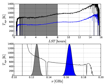
Figure 3.— (Top Panel) Band-averaged system temperature (Equation 8) as a function of local sidereal time for band I and II in black and blue, respectively. The shaded gray region indicates the range in local sidereal time used to compute the power spectra. (Bottom panel) Time-averaged system temperature, averaged over local sidereal times 1h00m to 8h00m. The shaded gray and blue regions show the window functions for Bands I and II, respectively. The persistent RFI mentioned in Section 3.1, as well as the band edges, appear as zeros in this estimate of of the system temperature.

Figure 3 shows the system temperature averaged over frequency and LST ranges used to compute the power spectra. Frequency- and time-averaged system temperatures for the bands centered at 124 MHz (hereafter Band I) and 164 MHz (Band II) are reported in Table 1.

3.6. Power Spectra

We compute the power spectrum using the delay spectrum approach (Parsons et al., 2012b). For short baselines, the delay transform of a visibility, defined as

$$\widetilde{V}(\tau)=\int V(\nu)e^{2\pi i\tau\nu}\ \mathrm{d}\nu$$ (9)

for visibility $V(\nu)$ and delay mode $\tau$, becomes an estimator for $T(\mathbf{k})$, the Fourier-transformed brightness temperature field. The power spectrum may be computed from the delay-transformed visibilities via the equation

$$P(\mathbf{k})=\left(\frac{\lambda^{2}}{2k_{B}}\right)^{2}\frac{X^{2}Y}{\Omega\Delta\nu}\left|\widetilde{V}(\tau)\right|^{2}.$$ (10)

Here, $P(\mathbf{k})$ is the three-dimensional power spectrum of 21 cm emission, $\lambda^{2}/2k_{B}$ is the conversion from Jy to K, $\Omega$ is the solid angle subtended by the primary beam, $\Delta\nu$ is the bandwidth of the observation, $X^{2}Y$ is the factor converting cosmological volume in $h^{-3}{\rm Mpc}^{3}$ to observed volume $\Omega\Delta\nu$ (taken from Equations 3 and 4 in Furlanetto et al. (2006)), and $\widetilde{V}(\tau)$ is the delay-transformed visibility. The $\mathbf{k}$ modes are determined by the baseline vector and the $\tau$ mode.

A subsequent covariance removal, described in detail in Appendix C of P14, projects the delay-transformed visibilities into a basis in which the covariance between two redundant baselines is diagonal, and then computes the power spectrum from the projected delay spectra. This procedure produces an estimate of the power spectrum for each LST bin and baseline type. To measure the uncertainties in the time-dependent power spectra, we bootstrap over both redundant baselines and LST samples.

3.7. Accounting for Ionospheric Effects

In P14 and J15, we ignored the effects of the ionosphere, since for Stokes $I$ these are largely changes in source position induced by refraction (for a recent study, see Loi et al., 2015) and these are negligible on the large angular scales considered (Vedantham & Koopmans, 2015, 2016). However, both spatial and temporal fluctuations in the Faraday depth of the Earth’s ionosphere will have a strong effect on polarized signal. As the total electron content (TEC) varies, it modulates the incoming polarized signal by some Faraday depth that is a function of both the TEC for that time and the strength of the Earth’s magnetic field. Though we assume that visibilities are redundant in LST for the purposes of averaging to form the power spectrum, they do in fact have variations due to the variable TEC of the ionosphere. Thus, averaging in LST could result in attenuation of signal. We are not able to directly image each day and calculate the effects of ionosphere variations based on the properties of celestial sources, but we are able to estimate the size of the effect on the visibilities used in the analysis of the power spectrum.

3.7.1 Characterizing Ionospheric Behavior over the Observing Season

Ionosphere data are provided by a number of sources. We have used data from the Center for Orbit Determination in Europe (CODE), whose global ionosphere maps are available in IONosphere map EXchange format (IONEX) via anonymous ftp. IONEX files from CODE are derived from $\sim$200 GPS sites of the International Global Navigation Satellite System Service (IGS) and other institutions. The time resolution of CODE data is 2 hours, and the vertical TEC values are gridded into pixels 5^∘ across in longitude, and 2.5^∘ in latitude.

We have used the core of the code provided from the ionFR package described in Sotomayor-Beltran et al. (2013, 2015) to access the IONEX files. As written, ionFR provides the RM toward a given RA as a function of UT at a given latitude (with the CODE two-hour time resolution interpolated into hourly values). We have generalized ionFR to calculate ionospheric RM values over a healpix sphere with nside=16 (the maximum spatial resolution obtainable from an IONEX file) using a custom-built python package radionopy.

For each day of the PSA32 campaign, we obtained the relevant IONEX file. For a fixed LST, we found the UT corresponding to that LST at transit for the PSA32 site for each day of observation. Using the data in an IONEX file and radionopy, we were able to calculate the vertical TEC and geomagnetic field (and hence RM) values over the entire hemisphere observed by PAPER. The result is a map of $\Phi(\Omega)$ giving the ionospheric RM $\Phi$ induced for sources in any direction; an example is shown in Figure 4.

[controls,loop,scale=0.45]3RM_2012-02-13_UT023

Figure 4.— Ionospheric RMs over the PSA32 site during 2012 February 13. Times are shown in UT (South African Standard Time is UT+2). The plot is shown in local horizon coordinates, with zenith at the center and the horizon around the edges. Note the large, smooth variation over the FoV. All of these RMs affect the measured visibilities, making accurate polarization calibration extremely difficult. The reader can view an animated hour-by-hour sequence by viewing this figure in adobe acrobat reader.

To give an indication of the time variability of the RM, as coadded into the power spectrum for that LST (recall Section 3.3), we calculated for each night of observation the zenith RM when three LSTs (4h, 6h, and 8h) were at transit. These are shown in Figure 5. Over the season, there is a large spread of ionospheric RMs for each LST. As the relevant phase shift of the Faraday-rotated spectrum is $\Phi\lambda^{2}$, this clearly varies by more than a radian over the range of days coadded. This will lead to a large attenuation of polarized power during LST-binning; we calculate this attenuation in the next section. Also note that there is a decrease in the average magnitude of the RM as LST increases. This is expected, given the strong correlation between the day / night cycle and TEC values (Radicella & Zhang, 1995; Tariku, 2015), and given that for this observing season, LST=4h corresponds to observing times shortly after sunset, while LST=8h is always well into the night.

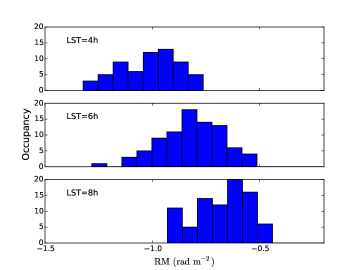
Figure 5.— From top to bottom, a histogram of the zenith ionospheric RMs over the season, for the transit of LSTs 4h, 6h and 8h. The large variance at any given LST corresponds to a large attenuation of polarized signal, as discussed in Section 3.7.2.

3.7.2 Calculating Ionospheric Attenuation of Polarized Signal

The effect of the ionosphere requires a modification of equation 2 to account for the effect of Equation 2, which following the formalism of Hamaker et al. (1996), is of the form

$$V^{\prime}_{I}=\int\mathrm{d}\Omega\,e^{-2\pi i\mathbf{b}\cdot\hat{s}\nu/c}[(A_{xx}+A_{yy})I+$$

$$(A_{xx}-A_{yy})(Q\cos\phi+U\sin\phi)]$$ (11)

where $\phi=2\Phi(\Omega)\lambda^{2}$ and $\Phi(\Omega)$ represents the spatial distribution of ionospheric rotation measures at the time of observation. As we have seen, $\Phi(\Omega)$ is a slowly varying function over the PAPER beam.

If we assumethat $\Phi(\Omega)$ is spatially constant, Equation 3.7.2 can be rewritten

$$V^{\prime}_{I} = \int\mathrm{d}\Omega\,e^{-2\pi i\mathbf{b}\cdot\hat{s}\nu/c}(A_{xx}+A_{yy})I$$ (12)

$$+ \cos\phi\int\mathrm{d}\Omega\,e^{-2\pi i\mathbf{b}\cdot\hat{s}\nu/c}(A_{xx}-A_{yy})Q$$

$$+ \sin\phi\int\mathrm{d}\Omega\,e^{-2\pi i\mathbf{b}\cdot\hat{s}\nu/c}(A_{xx}-A_{yy})U$$

$$\equiv {\cal V}_{I}+\cos\phi{\cal V}_{Q}+\sin\phi{\cal V}_{U}$$

and we can write the LST-averaged visibility as the Faraday rotation-weighted sum of otherwise redundant visibilities:

$$\widehat{V}=\frac{1}{N}\sum_{i}{\cal V}_{I}+\cos\phi_{i}{\cal V}_{Q}+\sin\phi_{i}{\cal V}_{U},$$ (13)

where $\phi_{i}$ is the zenith ionospheric Faraday depth from day $i$ and the other terms are the redundant component of the visibilities. Note that ${\cal V}_{I}$ does not provide contributions at high $k$ to the power spectrum due to the assumption of smooth-spectrum foregrounds, and we are concerned only with the leakage due to ${\cal V}_{Q}$ and ${\cal V}_{U}$. These visibilities’ contribution to the power spectrum for given LST will average approximately as

$$\widehat{P}\propto|\widehat{V}|^{2}=\frac{1}{N^{2}}\left(\sum_{i,j}e^{-2i(\Phi_{i}-\Phi_{j})\lambda^{2}}\right)|V|^{2}\equiv\varepsilon|V|^{2}.$$ (14)

The sum may be rewritten in terms of the $i=j$ components and the $j>i$ component:

$$\sum_{i,j}e^{-2i(\Phi_{i}-\Phi_{j})\lambda^{2}}=N+2\sum_{i>j}\cos\left\{2(\Phi_{i}-\Phi_{j})\lambda^{2}\right\}.$$ (15)

In the limit where all values of $\Phi_{i}$ are equal, this second term becomes $N(N-1)/2$, the number of $i,j$ pairs with $i>j$, showing that with no daily fluctuations in ionospheric Faraday depth, there is no change in the signal.

To estimate the level of ionospheric attenuation, we calculated $\varepsilon$ for the 3 LST transits described in the section above. For the observed distribution of RM at LST = 4h, 6h, 8h, the standard deviations of RM are $\sigma_{\Phi}=0.30,0.24,0.20$ rad m^-2 and the average attenuation was calculated to be $\varepsilon=0.42,0.41,0.48$ in Band II (164 MHz) and $\varepsilon=0.07,0.06,0.11$ in Band I (126 MHz), for each LST, respectively. To obtain some measure of the uncertainty in this value, we generated 10,000 realizations of the attenuation factor for an 82 day integration, drawing randomly from the RM distributions shown in Figure 5, and found the average simulated value to be $0.43\pm 0.06$ (Band II) and $0.07\pm 0.05$ (Band I). (Note that while we have neglected it, spatial variation in the TEC would tend to increase the attenuation.) The net effect is that polarized leakage into Stokes $I$ is notably decreased by this averaging process, as are the observed signals in Stokes $Q$ and $U$. A more sophisticated model of this leakage and attenuation is the subject of future work.

4. Results

4.1. Features of the Power Spectra

Figure 6 shows the power spectra resulting from the above analysis in $I$, $P\equiv Q+iU$ and $V$ as a function of LST for Band II. Figure 7 shows the LST average of these power spectra for Stokes $I$, $Q$, $U$ and $V$ in Bands I and II. Uncertainties in these power spectra are the bootstrap errors described in Section 3.6. The expected thermal noise sensitivity using the $T_{sys}$ computed from Section 3.5 and the sensitivity calculations of Parsons et al. (2012a) and Pober et al. (2014) are shown as dashed, cyan lines.

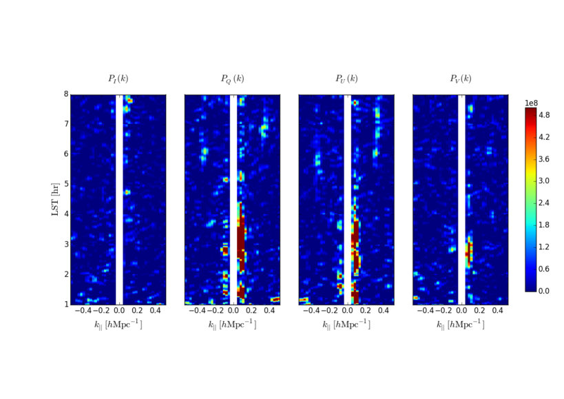
Figure 6.— Power spectra $P(k)$ from Band II, in units of ${\rm mK}^{2}\,h^{3}\,{\rm Mpc}^{-3}$, shown as a function of $k_{\parallel}$ and local sidereal time (LST) in hours, which is the same for all panels. $k_{\parallel}$ modes within the horizon for the 30 m baselines used are masked. From left to right, the panels show $P_{I}$, $P_{Q}$, $P_{U}$ and $P_{V}$. Features in these power spectra are discussed further in the text.

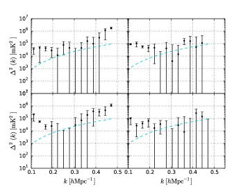
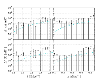
Figure 7.— Top: Spherically-averaged power spectra for the four Stokes parameters for Band I. Stokes $I$ is in the top left panel, $Q$ in the top right, $U$ in the lower left, and $V$ in the lower right. Error bars show 98% confidence intervals. Dashed, cyan lines indicate the theoretical level of thermal fluctuations, with $T_{sys}$ calculated in Section 3.5. Bottom: Same as the above, for Band II.

In Figure 6, we see that Band II Stokes $P_{I}$ and $P_{V}$ are largely devoid of features in LST. In the $P_{Q}$ and $P_{U}$ panels of Figure 6, there are two major features worth noting. The first is the excess of emission at $|k_{\parallel}|\lesssim 0.2\ h{\rm Mpc}^{-1}$, between right ascension 1h00m and 4h30m. That the excess exceeds the power in the corresponding $k$-bins of $P_{I}$ indicates that it is not due to leakage from Stokes $I$. It roughly corresponds in RA with the diffuse, polarized power shown in B13, which is evident between RA 22h and 3h, and takes its minimum value at around RA 5h. The low RM reported in B13 would mean that this emission would appear in our power spectra at low $k$, as observed. Whether this emission should be identified with the B13 features would require a true imaging analysis to establish.

The second feature of Figure 6 that we will comment on is the tracks of excess power in Q and U between RA 6h and 8h, with $|k_{\parallel}|\approx 0.35h{\rm Mpc}^{-1}$. Features such as these could be produced by polarized point sources of an apparent polarized flux of $\sim 1.5$ Jy observed through a Faraday screen with $\Phi\sim 60$ rad m^-2. Accounting for the ionospheric attenuation factor $\varepsilon$, the intrinsic polarized flux at 164 MHz would need to be $\sim 4$ Jy, and larger still if the sources did not pass through zenith (corresponding to RA 6h52m Dec -30°). While the features appear to transition between showing power in $P_{Q}$ and $P_{U}$, which would be expected for a intrinsically polarized point source undergoing parallactic rotation, the rotation between Q and U is faster in LST than expected for a celestial source. Nevertheless, to see whether there is a plausible bright source in this region, we refer to the results of Hurley-Walker et al. (2014). This survey covered 6100 square degrees, including the region above; excluding the brightest known sources (e.g., Pictor A, Fornax A), which do not match the position of the features, there are 22 sources with Stokes $I>10$ Jy in the primary beam of PAPER ($-52.5\arcdeg<\rm{Dec}<-7.5\arcdeg$) in that RA range, with the brightest being 28 Jy at 180 MHz. While it is not impossible that a source could be $>10\%$ polarized, the typical polarization fraction at these frequencies is much lower (Lenc et al., 2016). In addition to the point sources of Hurley-Walker et al. (2014), we also note that the Galactic Plane passes through zenith in this RA range. While the RM in the Plane is expected to be low, and the spectral smoothness of the primary beam is expected not to scatter power to high $k_{\parallel}$ (Kohn et al., 2016), it cannot be ruled out the strong Stokes $I$ power in the Plane couples to the instrument and produces these features. Other unidentified instrument systematics, which need not be constant in time as a result of changes in the instrument over the observing season, may also be responsible. However, using jackknife tests, for example, to test for this is difficult, because the feature is only 5.1$\sigma$, and thus unless the feature is highly localized in some portion of the data, partitioning the data would degrade the significance to $\sim 3\sigma$. We acknowledge that this anomaly merits further investigation, and that definitive identification as a celestial source requires a polarized imaging survey.

In Figure 7, the Stokes $I$ power spectra reproduce those of P14 and J15, as expected. Stokes $V$ is very nearly consistent with zero, except for the slight negative excess in the power spectrum at $k\sim 0.15$ (apparent as the missing point in the semi-log plot), which is clearly due to the bright (in absolute magnitude) feature at $0.05\,<\,k\,<\,0.15$ in the $P_{V}$ panel of Figure 6. It is not possible for astrophysical $V$ emission to produce a negative power spectrum, and thus this must represent a systematic artifact. It is evident that Band I is less consistent with zero than Band II (for all Stokes parameters), with the excess particularly notable for $k<0.2$. These features were noted by J15 for Stokes $I$ in the lower frequency band, and attributed to poorer cleaning of foreground power at lower frequencies and near the edge of the “wedge”.

4.2. Polarized Leakage into the EoR Power Spectrum

As discussed in Section 2, the dominant form of leakage of polarized power into $P_{I}$ in the analysis of the PAPER power spectrum comes from $Q\to I$ due to the primary beam ellipticity, as given in Equation 2. In general, calculating the fractional power leakage

$$\xi=\frac{|V_{Q}|^{2}}{|V_{I}|^{2}}$$ (16)

depends on knowing both the primary beam and the sky. We have done simulations to determine this factor in M13, but here we also develop an approximation that allows us to estimate $\xi$ knowing only the primary beam, under some assumptions about the source distribution on the sky.

We approximate $I$ and $Q$ as Gaussian, random fields with mean zero (as an interferometer, PAPER is insensitive to the mean value in any case). We also assume that $\langle Q^{2}\rangle\approx p^{2}\langle I^{2}\rangle$, that is, there is an average polarization fraction $p$ of Stokes $I$ relative to $Q$, where $p\ll 1$ (which is indeed true at higher frequencies; Tucci & Toffolatti, 2012). Under these assumptions, we can write the square of the visibility $V_{I}$, proportional to the measured $I$ spectrum, as

$$|V_{I}|^{2}=\mathcal{A}_{+}\otimes P_{I}+\mathcal{A}_{-}\otimes P_{Q},$$ (17)

where $P_{I}$ and $P_{Q}$ are the true power spectra of $I$ and $Q$, and $\otimes$ denotes a convolution. The weighting factors $\mathcal{A}_{\pm}$ are the contributions in power from the summed and differenced primary beams, defined as

$$\mathcal{A}_{\pm}\equiv\int|A_{xx}\pm A_{yy}|^{2}\ \mathrm{d}\Omega.$$ (18)

A similar expression to Equation 17 can be written for $V_{Q}$, with an interchange of $I$ and $Q$. Then

$$\xi=\frac{p^{2}\mathcal{A}_{+}+\mathcal{A}_{-}}{\mathcal{A}_{+}+p^{2}\mathcal{A}_{-}}\approx\frac{\mathcal{A}_{-}}{\mathcal{A}_{+}}.$$ (19)

This ratio, when multiplied by the measured $P_{Q}$ can be used as a metric to characterize the level of polarization leakage present in a measurement of $P_{I}$. Table 1 shows the value of this ratio for the PAPER beam (Pober et al., 2012) for the two bands. The ratio can also be calculated from simulations, and on average agrees well with the simpler estimate of Equation 19.

The level of leakage predicted by Equation 19 shows that in the lowest $k_{\parallel}$ bins, the $I$ power spectrum of P14 and J15 cannot be dominated by $Q\to I$ leakage. The levels of polarized leakage are, to order of magnitude, $10^{3}\ {\rm mK}^{2}$ in Band I, and $10^{2}\ {\rm mK}^{2}$ in Band II. The lack of a detection of polarized power (Stokes $Q$ and $U$) in Figure 7 is consistent with what is known about polarized emission, combined with the attenuation factor from the ionosphere in Section 3.7.2. Because we are considering only $k_{\parallel}>0.15~{}h~{}\rm{Mpc}^{-1}$, we assume the contribution of low-RM diffuse emission is negligible (a result corroborated by Kohn et al. (2016), who probe a much greater range of $k$-values over a comparatively short integration with the PAPER polarized imaging array). For point sources, a polarized fraction $p_{rm150~{}MHz}=0.006$ (lower than that assumed in M13) would be consistent with the single reported point source in B13 and an interpretation of the results of Asad et al. (2015). When combined with the ionospheric attenuation, this would produce a power spectrum below our limits, and leakage well below the excess present in the lowest $k_{\parallel}$ bins of the $P_{I}$ power spectra in P14 and J15. Indeed, if these levels are typical, leakage would be below the levels reported in the more recent PAPER-64 results of Ali et al. (2015), albeit under different ionospheric conditions.

5. Conclusion

We have presented the first limits on the power spectra of all four Stokes parameters in two frequency bands, centered at 126 MHz ($z=10.3$) and 164 MHz ($z=7.66$). These data come from from a three-month observing campaign of a 32-antenna deployment of PAPER. These power spectra are processed in the same way as the results on the unpolarized power spectrum have been reported at $z=7.7$ (Parsons et al., 2014) and $7.5<z<10.5$ (Jacobs et al., 2015). We do not find a a definitive detection of polarized power. The limits are sufficiently low, however, that the level of polarized leakage present in previous PAPER measurements must be less than 100 mK² at $k_{\parallel}\sim 0.2\ h{\rm Mpc}^{-1}$, below the excess found in those measurements.

We additionally find that that the variation in ionospheric RM is sufficient to attenuate the linearly polarized emission in these measurements by factors between 2.5 and 16, depending on the observing frequency. Combined with a lower polarized fraction for point sources than assumed in Moore et al. (2013), this is consistent with our nondetection of polarized power.

PAPER in the grid array configuration presented here is incapable of creating the images with high dynamic range needed to isolate polarized emission. Future work will explore in more detail the effect of the ionosphere and the full degree of depolarization present in long EoR observing seasons, as well as the full effects of polarized leakage from wide-field beams and polarization calibration.

References

- Ali et al. (2015) Ali, Z. S., Parsons, A. R., Zheng, H., et al. 2015, ApJ, 809, 61
- Asad et al. (2015) Asad, K. M. B., Koopmans, L. V. E., Jelić, V., et al. 2015, MNRAS, 451, 3709
- Bernardi et al. (2009) Bernardi, G., de Bruyn, A. G., Brentjens, M. A., et al. 2009, A&A, 500, 965
- Bernardi et al. (2013) Bernardi, G., Greenhill, L. J., Mitchell, D. A., et al. 2013, ApJ, 771, 105
- Carozzi & Woan (2009) Carozzi, T. D., & Woan, G. 2009, MNRAS, 395, 1558
- Cohen et al. (2004) Cohen, A. S., Röttgering, H. J. A., Jarvis, M. J., Kassim, N. E., & Lazio, T. J. W. 2004, ApJS, 150, 417
- Cotton (2012) Cotton, W. D. 2012, Journal of Astronomical Instrumentation, 1, 50001
- Farnes et al. (2014) Farnes, J. S., Gaensler, B. M., & Carretti, E. 2014, ApJS, 212, 15
- Furlanetto et al. (2006) Furlanetto, S. R., Oh, S. P., & Briggs, F. H. 2006, Phys. Rep., 433, 181
- Geil et al. (2011) Geil, P. M., Gaensler, B. M., & Wyithe, J. S. B. 2011, MNRAS, 418, 516
- Gießübel et al. (2013) Gießübel, R., Heald, G., Beck, R., & Arshakian, T. G. 2013, A&A, 559, A27
- Hales et al. (1988) Hales, S. E. G., Baldwin, J. E., & Warner, P. J. 1988, MNRAS, 234, 919
- Hamaker et al. (1996) Hamaker, J. P., Bregman, J. D., & Sault, R. J. 1996, A&AS, 117, 137
- Harris (1978) Harris, F. J. 1978, IEEE Proceedings, 66, 51
- Hurley-Walker et al. (2014) Hurley-Walker, N., Morgan, J., Wayth, R. B., et al. 2014, PASA, 31, 45
- Jacobs et al. (2013) Jacobs, D. C., Parsons, A. R., Aguirre, J. E., et al. 2013, ApJ, 776, 108
- Jacobs et al. (2015) Jacobs, D. C., Pober, J. C., Parsons, A. R., et al. 2015, ApJ, 801, 51
- Jelić et al. (2010) Jelić, V., Zaroubi, S., Labropoulos, P., et al. 2010, MNRAS, 409, 1647
- Jelić et al. (2014) Jelić, V., de Bruyn, A. G., Mevius, M., et al. 2014, A&A, 568, A101
- Kohn et al. (2016) Kohn, S. A., Aguirre, J. E., Nunhokee, C. D., et al. 2016, ApJ, 823, 88
- La Porta & Burigana (2006) La Porta, L., & Burigana, C. 2006, A&A, 457, 1
- Lenc et al. (2016) Lenc, E., Gaensler, B. M., Sun, X. H., et al. 2016, ApJ, 830, 38
- Liu et al. (2010) Liu, A., Tegmark, M., Morrison, S., Lutomirski, A., & Zaldarriaga, M. 2010, MNRAS, 408, 1029
- Loi et al. (2015) Loi, S. T., Murphy, T., Bell, M. E., et al. 2015, MNRAS, 453, 2731
- Mathewson & Milne (1964) Mathewson, D. S., & Milne, D. K. 1964, Nature, 203, 1273
- Mathewson & Milne (1965) —. 1965, Australian Journal of Physics, 18, 635
- Moore et al. (2013) Moore, D. F., Aguirre, J. E., Parsons, A. R., Jacobs, D. C., & Pober, J. C. 2013, ApJ, 769, 154
- Morales et al. (2006) Morales, M. F., Bowman, J. D., & Hewitt, J. N. 2006, ApJ, 648, 767
- Morales et al. (2012) Morales, M. F., Hazelton, B., Sullivan, I., & Beardsley, A. 2012, ApJ, 752, 137
- Mulcahy et al. (2014) Mulcahy, D. D., Horneffer, A., Beck, R., et al. 2014, A&A, 568, A74
- Oppermann et al. (2012) Oppermann, N., Junklewitz, H., Robbers, G., et al. 2012, A&A, 542, A93
- Parsons et al. (2012a) Parsons, A., Pober, J., McQuinn, M., Jacobs, D., & Aguirre, J. 2012a, ApJ, 753, 81
- Parsons & Backer (2009) Parsons, A. R., & Backer, D. C. 2009, AJ, 138, 219
- Parsons et al. (2012b) Parsons, A. R., Pober, J. C., Aguirre, J. E., et al. 2012b, ApJ, 756, 165
- Parsons et al. (2014) Parsons, A. R., Liu, A., Aguirre, J. E., et al. 2014, ApJ, 788, 106
- Pen et al. (2009) Pen, U. L., Chang, T. C., Hirata, C. M., et al. 2009, MNRAS, 399, 181
- Pober et al. (2012) Pober, J. C., Parsons, A. R., Jacobs, D. C., et al. 2012, AJ, 143, 53
- Pober et al. (2013) Pober, J. C., Parsons, A. R., Aguirre, J. E., et al. 2013, ApJ, 768, L36
- Pober et al. (2014) Pober, J. C., Liu, A., Dillon, J. S., et al. 2014, ApJ, 782, 66
- Radicella & Zhang (1995) Radicella, S. M., & Zhang, M. L. 1995, Annals of Geophysics, 38
- Shaw et al. (2015) Shaw, J. R., Sigurdson, K., Sitwell, M., Stebbins, A., & Pen, U.-L. 2015, Phys. Rev. D, 91, 083514
- Sotomayor-Beltran et al. (2013) Sotomayor-Beltran, C., Sobey, C., Hessels, J. W. T., et al. 2013, A&A, 552, A58
- Sotomayor-Beltran et al. (2015) —. 2015, A&A, 581, C4
- Spoelstra (1984) Spoelstra, T. A. T. 1984, A&A, 135, 238
- Sutinjo et al. (2015a) Sutinjo, A., O’Sullivan, J., Lenc, E., et al. 2015a, Radio Science, 50, 52
- Sutinjo et al. (2015b) Sutinjo, A. T., Colegate, T. M., Wayth, R. B., et al. 2015b, IEEE Transactions on Antennas and Propagation, 63, 5433
- Tariku (2015) Tariku, Y. A. 2015, Earth, Planets and Space, 67, 1
- Tucci & Toffolatti (2012) Tucci, M., & Toffolatti, L. 2012, Advances in Astronomy, 2012, arXiv:1204.0427
- Vedantham & Koopmans (2015) Vedantham, H. K., & Koopmans, L. V. E. 2015, MNRAS, 453, 925
- Vedantham & Koopmans (2016) —. 2016, MNRAS, 458, 3099
- Westerhout et al. (1962) Westerhout, G., Seeger, C. L., Brouw, W. N., & Tinbergen, J. 1962, Bull. Astron. Inst. Netherlands, 16, 187