Orientational hysteresis in swarms of active particles in external field

Abstract

Structure and ordering in swarms of active particles have much in common with condensed matter systems like magnets or liquid crystals. A number of important characteristics of such materials can be obtained via dynamic tests such as hysteresis. In this work, we show that dynamic hysteresis can be observed also in swarms of active particles and possesses similar properties to the counterparts in magnetic materials. To study the swarm dynamics, we use computer simulations of the active Brownian particle model with dissipative interactions. The swarm is confined to a narrow linear channel and the one-dimensional polar order parameter is measured. In an oscillating external field, the order parameter demonstrates dynamic hysteresis with the shape of the loop and its area varying with the amplitude and frequency of the applied field, swarm density and the noise intensity. We measure the scaling exponents for the hysteresis loop area, which can be associated with the controllability of the swarm. Although the exponents are non-universal and depend on the system’s parameters, their limiting values can be predicted using a generic model of dynamic hysteresis. We also discuss similarities and differences between the swarm ordering dynamics and two-dimensional magnets.

1 Introduction

Hysteresis is a nonlinear phenomenon commonly observed in various metastable systems, which have more than one internal state krasnoselskii.ma:1989 . In such systems, the response to a change of the environment depends on the history of this environment. Although the most prominent example of hysteresis is a magnetisation response of a ferromagnet in an oscillating field lyuksyutov.i:1999 , this effect is not limited to only ferromagnetic or ferroelectric materials. Hysteresis is also observed in various physical, mechanical, chemical, biological and ecological systems. In active systems chate.h:2008 ; couzin.id:2002 ; ihle.t:2013 hysteresis of the collective motion states has been shown to arise near the point of orientational phase transition, where system is most sensitive to any changes in fluctuation strength.

While the interest in hysteretic effects is driven mostly by practical applications in electronics and engineering, hysteresis occurring in many-body systems is an intriguing fundamental problem on itself chakrabarti.bk:1999 ; reimann.p:1999 . Although the phenomenon has been known for several hundreds of years, the systematic study of hysteresis has started only in the last quarter of the twentieth century krasnoselskii.ma:1989 .

In this study, we explore the dynamic hysteresis in swarms of active species using the magnetic analogy. This analogy is based on the ability of active swarms to reach orientationally ordered states, similar to those in ferromagnets vicsek.t:1995 ; vicsek.t:2012 ; czirok.a:1999 ; toner.j:1995 ; toner.j:1998 ; toner.j:2005 ; ramaswami.s:2010 . The transition from a disordered state of a swarm of interacting active particles to an ordered state happens upon reduction of noise at fixed propulsion speed. The common polar order parameter for the swarm, the mean particle velocity, measured as a function of the noise amplitude, behaves in the same way as the magnetisation vector in magnetic materials upon the variation of temperature toner.j:2005 ; ramaswami.s:2010 . The similarity between swarms and magnets is not limited to the behaviour of the mean order parameter but covers a wide range of more subtle properties such as the spatial correlations (two-point correlation function), susceptibility, and the divergence of the correlation radius at the critical point czirok.a:1999 ; baglietto.g:2008 ; romenskyy.m:2013 ; cavagna.a:2010 . The ideas from lattice models of magnets such as Heisenberg model and Ising model have been successfully applied to describe swarm dynamics czirok.a:1999 ; solon.ap:2013 .

We hope to extend the analogy between the equilibrium condensed matter and active swarms to dynamic properties. Although the interaction of active swarms with external fields has not been extensively studied so far, it is easy to envision that an orienting field would have the same effect on a swarm that is observed in magnetic systems. In particular, as the swarm has a finite orientation relaxation time, there must be a room for dynamic hysteresis controlled by a competition of the external drive and the internal relaxation. Therefore, one can attempt to characterise the swarm dynamics by retentivity, the ability to align in absence of the field, coercivity, the magnitude of field in the opposite direction needed to revert the direction of motion of the swarm, and susceptibility, the intensity of the response of the swarm to the action of field. In addition, one can hope to learn the main relaxation times, for example the time needed to reorient the swarm, and estimate the strength and the frequency of the required controlling signals. All these quantities can become extremely useful if we try to control the collective dynamics in either robotic swarms, human crowds or groups of animals in a farm or in Nature.

The remainder of the paper is organised as follows: Section 2 describes the active Brownian particle model with interactions and simulation settings, Section 3 presents the results on orientational ordering in the active swarm, Section 4 presents the discussion of our main observations, and Section 5 concludes the paper.

2 Model and simulation setup

To study the orientational hysteresis in an active swarm, we use a two-dimensional system of active Brownian particles (ABP) ebeling.w:1999 ; ebeling.w:2000 with dissipative interactions. Motion of the agents is confined into a narrow straight channel with periodic boundaries in the long direction and purely repulsive walls in the short direction. The ABP-DI model is able to produce a globally aligned phase if the energy influx rate is sufficiently high and the interactions are sufficiently strong lobaskin.v:2013 .

Our implementation of the ABP-DI is as described in our previous works lobaskin.v:2013 ; romensky.m:2014 . The particle motion is governed by the Langevin equation

$$m\frac{d\mathbf{V}_{i}}{dt}=\mathbf{F}_{i}$$ (1)

where $m$ is the particle mass (set to unity in this work) and $\mathbf{V}_{i}$ is the velocity of particle $i$. The total force $\mathbf{F}_{i}(t)$ acting on each particle is given by:

$$\mathbf{F}_{i}=\mathbf{F}_{i}^{S}-\gamma^{E}\mathbf{V}_{i}+\mathbf{F}^{T}_{i}+\sqrt{2D^{E}}{\bm{\xi}_{i}}(t)+\mathbf{H}(t)$$ (2)

where $\mathbf{F}_{i}^{S}$ is the force that comes from interactions within the swarm, $\gamma^{E}$ is the coefficient of viscous friction, which is set by the properties of the environment, $\mathbf{F}^{T}_{i}$ is the thrust term. The term $\sqrt{2D^{E}}{\bm{\xi}}_{i}(t)$ is the random force of strength $D^{E}$ and $\bm{\xi}(t)$ is representing a Gaussian white noise with zero-mean and unit variance. The strength of the noise is set by the fluctuation-dissipation relation at the ambient temperature $T^{E}$

$$D^{E}=\frac{k_{B}T^{E}}{(\gamma^{E})^{3}}.$$ (3)

The thrust term has the form:

$$\mathbf{F}_{i}^{T}=\frac{dq}{c+dV_{i}^{2}}\mathbf{V}_{i}$$ (4)

where $d$ is the constant determining the rate of conversion of internal energy into kinetic energy, $c$ is the parameter controlling energy loss, and $q$ is the constant determining the gain of energy from the environment. In a stationary state, motion of each particle is characterized by velocity $V_{0}^{2}$, which is defined through the system’s parameters as

$$V_{0}^{2}=\frac{q}{\gamma^{E}}-\frac{c}{d}$$ (5)

at $q>\gamma^{E}c/d$ ebeling.w:1999 ; romanczuk.p:2012 .

$\mathbf{F}_{i}^{S}(t)$ is the force coming from the interactions within the swarm, which describes inelastic collisions between the particles according to the Dissipative Particle Dynamics (DPD) method espanol.p1:1995 .

The dissipative force is taken in the form of a friction force applied to the component of the motion in the direction of the particle connecting vector. It generally consists of three parts:

$${\mathbf{F}_{i}^{S}=\sum\limits_{j\neq i}(\mathbf{F}_{ij}^{C}+\mathbf{F}_{ij}^{D}+\mathbf{F}_{ij}^{R})}$$ (6)

where $\mathbf{F}_{ij}^{C}$, $\mathbf{F}_{ij}^{D}$, and $\mathbf{F}_{ij}^{R}$ represent the conservative, dissipative, and random forces between particles $i$ and $j$, respectively. The conservative force reflects the excluded volume interactions:

$${\mathbf{F}_{ij}^{C}=\begin{cases}G\left(1-\displaystyle\frac{r_{ij}}{r_{r}}\right)\hat{\mathbf{r}}_{ij},&r_{ij}\leq r_{r}\\ 0,&r_{ij}>r_{r}\end{cases}}$$ (7)

where $\mathbf{r}_{ij}=\mathbf{r}_{i}-\mathbf{r}_{j}$ is the distance between particles $i$ and $j$, $r_{ij}=|\mathbf{r}_{ij}|$ is its magnitude, $\hat{\mathbf{r}}_{ij}=\mathbf{r}_{ij}/r_{ij}$ is the unit vector from $j$ to $i$, $G$ is a parameter determining the maximum repulsion between the particles, $r_{r}=r_{c}/2$ is the radius of the repulsion zone, and $r_{c}$ is the cut-off distance of the interaction.

The dissipative force punishes the velocity differences between the neighbouring particles and, therefore, provides a mechanism of relaxation of the velocity field towards the stationary state. We take it in the form of a friction force applied to the component of the relative motion in the direction of the particle connecting vector lobaskin.v:2013 , i.e. a velocity adjustment for particles following one another.

$${\mathbf{F}_{ij}^{D}=-\gamma^{S}\omega(r_{ij})(\hat{\mathbf{r}}_{ij}\cdot\mathbf{V}_{ij})\hat{\mathbf{r}}_{ij}}$$ (8)

The pairwise friction coefficient $\gamma^{S}$ determines the degree of inelasticity of the collisions, and $\omega(r)$ is a weight function that describes the particle’s “soft shell”:

$${\omega(r)=\begin{cases}\left(1-\displaystyle\frac{r_{ij}}{r_{c}}\right)^{2},&r_{ij}\leq r_{c}\\ 0,&r_{ij}>r_{c}\end{cases}}$$ (9)

We neglect the random pairwise force $\mathbf{F}_{ij}^{R}$ in this work.

The external field $\mathbf{H}(t)$ in our model is set by

$${\mathbf{H}(t)=H_{0}\sin{(\omega t)}\hat{\mathbf{x}}}$$ (10)

where $H_{0}$ is the amplitude of the periodic field, $\omega=2\pi f$ is the angular frequency, and $\hat{\mathbf{x}}$ is the unit vector pointing along the x-axis.

Since the periodic force acts only along one axis, the natural order parameter for our system is the mean one-component velocity $V_{x}$

$${\varphi(t)=\frac{1}{N}\sum_{i=1}^{N}V_{ix}(t)}$$ (11)

We used non-normalised order parameter in the study of the hysteresis loops. To study the phase behaviour of the swarm in absence of the field, we normalised the order parameter to bring it into the range from 0 to 1 as follows

$${\varphi_{n}=\left\langle\frac{\left|\frac{1}{N}\sum_{i=1}^{N}V_{ix}(t)\right|}{\frac{1}{N}\sum_{i=1}^{N}{V}_{i}(t)}\right\rangle},$$ (12)

where $\langle\cdot\rangle$ stands for ensemble average. To locate the phase transition points precisely we calculated the Binder cumulant binder.k:1981 using the normalised order parameter defined by Eq. (12)

$$G_{L}=1-\frac{\langle\varphi^{4}_{L}\rangle_{t}}{3\langle\varphi^{2}_{L}\rangle^{2}_{t}}$$ (13)

where $\langle\cdot\rangle_{t}$ stands for the time average and index $L$ denotes the value calculated for a system of linear length $L$. The Binder cumulant has a very weak dependence on the system size so $G_{L}$ takes a universal value at the critical point for any $L$ if the density $\rho$ and the energy influx rate $q$ are kept constantchate.h2:2008 . In this work, the transition points in $q-\rho$ plane are, therefore, defined as an intersection between the three $G_{L}-q$ curves for different channel length $L$ at constant density. Those points were then used to construct the phase diagram.

The area of hysteresis loops has been calculated as

$${A=\oint\varphi(H)dH}$$ (14)

The system relaxation time $\tau$ was measured from the order parameter relaxation dynamics towards the steady state $\varphi_{\infty}$ at fixed $\rho$, $q$, $T^{E}$, and $H_{0}$

$${\varphi(t)=\varphi_{\infty}\left(1-e^{-(t-t_{0})/\tau}\right)}.$$ (15)

upon application of a step-like signal at time $t_{0}$:

$$H(t)=\begin{cases}H_{0},&t\geq t_{0}\\ 0,&t<t_{0}\end{cases}.$$ (16)

Examples of the order parameter relaxation in constant field are shown in Fig. 1. Dependence of the relaxation time $\tau$ on the strength of applied field $H_{0}$ and temperature $T^{E}$ is presented in Fig. 2.

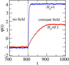
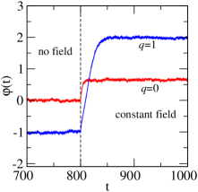
Figure 1: Dynamics of the orientational order parameter $\varphi$ in the ABP-DI system subjected to a constant field ($\rho=0.04$, $T^{E}=0.3$). The field is switched on at $t_{0}=800$. (a) Varying $H_{0}$, $q=1$ . (b) Varying $q$, $H_{0}=0.2$.

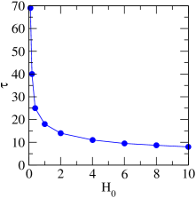
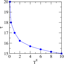
Figure 2: Relaxation time of the orientational order parameter $\varphi$ in the ABP-DI system subjected to a constant field ($\rho=0.04$, $q=1$). Each point represents an average over five independent runs. (a) Varying $H_{0}$, $T^{E}=0.3$ . (b) Varying $T^{E}$, $H_{0}=1$.

All simulations were performed with the following set of key parameters: $\gamma^{E}=0.3$, $G=1$, $d=2$, $c=0.8$, $\gamma^{S}=0.3$, $r_{c}=2$ (cut-off radius), $r_{r}=1$ (the particle radius of repulsion). The radius of repulsion of the particles sets the unit of length if the simulation system. To set the unit of time, we choose a unit speed $v=1$ such that a particle moving at $V=v$ would make a distance $r_{r}$ per unit time. This definition can be reformulated in terms of kinetic energy: our simulation units are such that an active particle moving at a speed of one body radius per unit time would have a kinetic energy $E=mV^{2}/2=1/2$. Therefore, a temperature $T^{E}=0.3$ in our settings, which sets the noise amplitude, means that the root-mean-square speed of particles without propulsion ($q=0$) is $V_{\text{rms}}=\sqrt{T^{E}/m}=0.548$, i.e. 0.548 body radii per unit time.

Simulations were performed with time step of $\Delta t=0.01$. The positions of the agents were propagated using the Verlet algorithm verlet.l:1967 . The geometric confinement was represented by the linear channel with its walls lying along the x-axis and periodic boundaries in the x-direction. Dimensions of the channel were fixed at $50\times 500$ units for all runs (unless stated otherwise). Repulsions from the channel walls were modeled as mirror-like reflections: after bouncing off the wall the component of the particle velocity normal to the wall was getting the opposite sign while the tangential one was kept unchanged. In all our simulations the oscillating field was applied parallel to the confining walls. Initial positions of particles have been chosen at random in all simulations. Total number of time steps has been set in the region $2\times 10^{6}$ - $1\times 10^{8}$ depending on the frequency of the external field and the hysteresis loops were averaged over at least 10 cycles.

3 Results

3.1 Orientational ordering

As we found in our previous work, an ABP-DI swarm is known to order orientationally in free space at sufficiently high density, strong interactions (as expressed by $F^{S}$), and/or strong propulsion lobaskin.v:2013 . We observe the same behaviour in confinement. A few typical snapshots of the part of the system are shown in Figs. 3 and 4. The distribution of the active particles along and across the channel is visibly affected by their incoming power $q$ (see Fig. 3) and by the number density $\rho$ (see Fig. 4). While at low incoming energy rates the particles behave like a gas with not much correlation in their motion, at certain critical level of energy pumping their motion becomes orientationally ordered. Another obvious result of increasing the incoming power is the particle aggregation. As we see in Fig. 3b, already at $q=1$ we observe significant density fluctuations and at $q=10$ large compact clusters appear. A similar effect is observed on increasing particle number density $\rho$: at low density $\rho=0.04$ (Fig. 4a) we see only gas-like behaviour and disordered motion, while at higher densities $\rho=0.1$ and $\rho=0.4$ both the aggregation and alignment become pronounced.

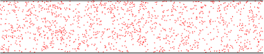
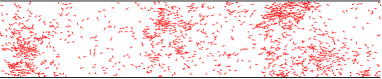
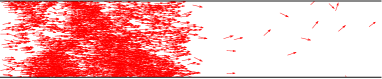
Figure 3: Simulation snapshots (cutout of the full simulation box) of swarms for the ABP-DI model in a linear channel confinement at various energy input rate $q$ ($\rho=0.1$, $T^{E}=0.3$). (a) $q=0$. (b) $q=1$. (c) $q=10$. Arrows indicate the direction of motion of the individuals as well as the magnitudes of the velocities.

In Fig. 5a we plot the polar order parameter as a function of the energy influx rate for various densities. It is clearly seen from the graph that the ABP-DI model confined to a linear channel displays a phase transition to a polarly ordered state upon increase of the input power. The graph also presents a clear evidence of a first order phase transition, when the phase transformation is discontinuous (as confirmed by the standard Binder cumulant analysis). For low densities, $\rho=0.04-0.06$, we observe large jumps in the value of $\varphi_{n}$ from almost 0 in disordered state to $0.33$ when the order is formed. We should also note that the transition happens earlier for more dense systems. To illustrate the phase behaviour of the system along the density path we plot $\varphi_{n}$ as a function of $\rho$ in Fig. 5b. The variation of the order parameter indicates a discontinuous phase transition on increasing the density. Noteworthy, the order parameter jump becomes smaller at higher densities and lower energy influx rates.

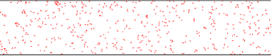
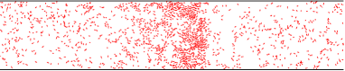
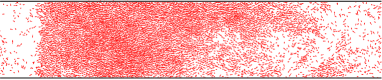
Figure 4: Simulation snapshots (cutout of the full simulation box) of swarms for the ABP-DI model in a linear channel confinement at various density $\rho$ ($q=0.5$, $T^{E}=0.3$). (a) $\rho=0.04$. (b) $\rho=0.1$. (c) $\rho=0.4$. Arrows indicate the direction of motion of the individuals as well as the magnitudes of the velocities.

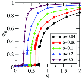
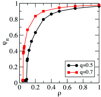
Figure 5: Normalised order parameter for the ABP-DI system in absence of external field, $H_{0}=0$: (a) the iso-$\rho$ curves and (b) the iso-$q$ curves.

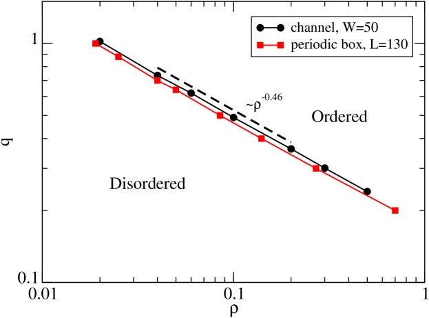
Figure 6: Phase diagram of the ABP-DI model in absence of external field, $H_{0}=0$, in confinement with channel width $W=50$ and in a periodic square simulation box of linear size $L=130$.

The ordering in the confined system is also affected by the transverse size of the channel. In Fig. 6 we present the phase diagram for the ABP-DI model in channel confinement in coordinates $\rho-q$. We observe practically the same power law as in the unbounded space, $q_{c}\propto\rho_{c}^{-0.46}$ romenskyy.m:2013 . In the whole range of explored densities and the input power, the transition is of the first order. The discontinuous nature of the transition is related to formation of density waves, which can be seen in the snapshots in Figs. 3 and 4. This issue is discussed in more detail in our paper on the Vicsek model romensky.m:2014a .

3.2 Hysteresis of the mean velocity of the swarm

To steer the swarm motion, we now apply a homogeneous oscillating field, which exerts a force $H(t)$ on the particles along the channel. In simulations, we vary the field oscillation amplitude $H_{0}$ and frequency $f$. The system parameters are set so that the swarm is orientationally ordered in absence of field. To compare different systems, we will further present the frequency in dimensionless form, scaled by the order parameter relaxation time $\tau$, which is defined by Eq. (15).

Figure 7 shows the measured values of the orientational order parameter as a function of time together with the corresponding field variation curves. At low frequencies, $f\tau=0.1$, we see that the velocity of the swarm is not proportional to the field although it changes in phase with the latter. At $f\tau=1$ the variation of $\varphi$ becomes sinusoidal but now exhibits a phase lag as compared to the field variation. At the highest frequency, $f\tau=10$ the order parameter does not change the sign but rather oscillates about a fixed non-zero value $|\varphi|\approx 0.83$. This value, however, is different from that observed in the absence of a driving field $|\varphi|\approx 0.96$. The corresponding $H-\varphi$ diagrams are presented in Fig. 8. The shape of the loops changes from sigmoidal at low frequency, $f\tau=0.1$ , where the curve is also symmetric with respect to the change of sign of the field, to an ellipsoidal one at higher frequencies, $f\tau=0.5$, $2.5$ and $25$. At high frequencies, as we noted before, the order parameter does not change the sign within the cycle, and the loops are not symmetric with respect to the origin.

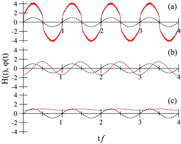
Figure 7: Variation of the order parameter for the ABP-DI swarm at three different frequencies of the driving field: (a) $f\tau=0.1$. (b) $f\tau=1$. (c) $f\tau=10$. Other parameters: $\rho=0.04$, $T^{E}=0.3$, $H_{0}=1$. The order parameter values $\varphi(t)$ are shown by the solid lines while the field $H(t)$ by the dashed curves. The upper set of curves (a) corresponds to the slow field variation, such that the swarm has time to relax to the steady state and is always in phase with the field. The lower one (c) corresponds to fast field variation, such that the swarm has no chance to follow the field and reorient itself completely. Note that the time axis in each subplot is scaled by the corresponding field oscillation period.

To illustrate the microscopic dynamic properties of the active particles, we plotted the instantaneous velocity histograms along with the instantaneous values of the field and the order parameter in Fig. 9. The motion is clearly polarised at $f\tau\approx 0,0.25$, 0.5, 0.75, and 1.0. The polarisation is strongest at $f\tau\approx 0.25$ and 0.75. At the points $f\tau=0.1$ and 0.6, where the order parameter $\varphi(t)=0$, we see characteristic crater-like distributions with velocity peaks along the $y$-axis. Therefore, the states with zero average velocity are achieved not by reduction of individual velocities but rather by loss of polarisation, when the particles are not braking to reverse the direction of motion but making an U-turn. Therefore, at some moments we can see them moving predominantly across the channel.

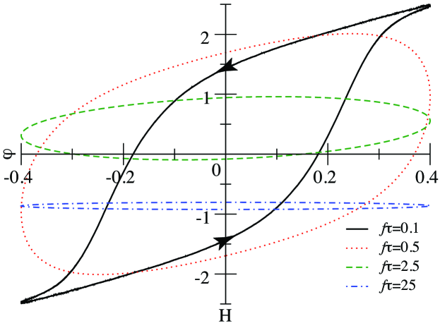
Figure 8: Typical $H-\varphi$-diagrams for the ABP-DI swarm at different frequencies of the driving field. Other parameters: $\rho=0.04$, $T^{E}=0.3$, $H_{0}=0.4$.

.

All the loop shapes we observe here are quite familiar from the magnetic hysteresis mayergoyz.id:1991 ; huang.z:2005 ; vatansever.e:2013 . At low frequencies, where the hysteresis loop is sigmoidal, we measured the dynamic characteristics of the swarm, which quantify its controllability. The dynamic coercivity – half-width at middle section – as can be seen in Fig. 10a,c,e, grows with the field frequency, field amplitude, but decreases with temperature. The coercivity vanishes in the static limit but grows as $H_{c}\propto f^{0.55}$ with the frequency. The resistance of the swarm to the action of the re-orienting field is related to the persistence of the particle motion and orienting action of the channel. In confinement, however, when the transverse size of the swarm is large enough, there exists a kinetic barrier for reorientation due to aligning action of the walls, which can prevent the reorientation and lead to long-living aligned states even in the presence of opposing fields. We were not able to observe static hysteresis at the chosen conditions, as the swarm always did reorient in the end in a constant field. We can envision, however, that in narrower channels and at higher density such that the cluster is system-spanning the system can demonstrate static hysteresis. In Fig. 10b,d,f, we see that the dynamic remanence – the residual polarisation of the swarm when the field turns zero – also grows with frequency and field amplitude, but decreases with temperature. In the limit of $f\to 0$, the dynamic remanence simply reflects the stationary value of the mean swarm velocity without the field while the coercivity turns zero. At higher frequencies, however, it is impossible to determine these characteristics due to completely different shape of the loops. Both properties contribute to the integral characteristic of hysteretic systems, the area of the loop, which thus reflects the system’s overall dynamic controllability (or rather agreeability in this context) in the low frequency region. In a perfectly controlled system, such that the mean velocity is always in phase with the external field, the loop area turns zero. In contrast, a large loop area indicates the “amount of disagreement” between the field and the order parameter. At high frequencies, the field variation is too fast for the particles and their velocity hardly varies at all but rather oscillates around the initial value. The particles cannot accelerate enough. The faster the field the less they catch, so the loops ar getting flatter and flatter. In this region, however, it cannot be easily interpreted in terms of agreeability, as the particles are moving opposite to the field direction half of the time at any $f\tau>1$.

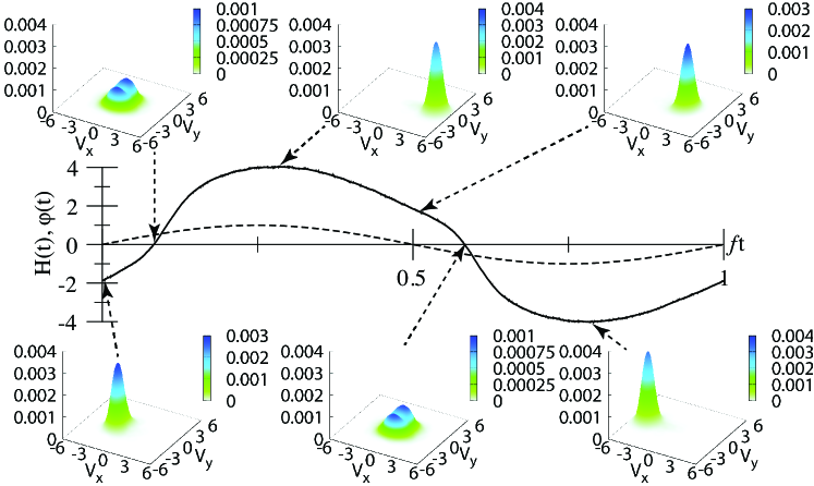
Figure 9: Variation of the particle velocity distributions within the field oscillation cycle. System parameters: $\rho=0.04$, $T^{E}=0.3$, $H_{0}=1$, $f\tau=0.18$. The order parameter values $\varphi(t)$ are shown by the solid line while the field $H(t)$ by the dashed curve.

.

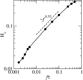
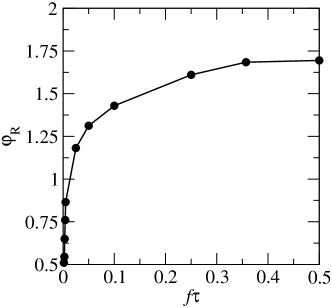
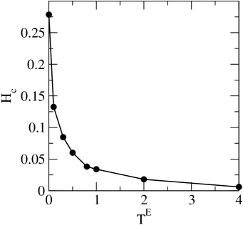
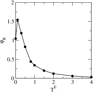
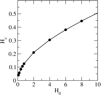
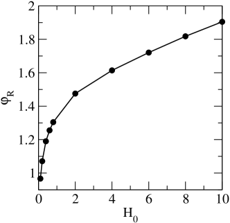
Figure 10: The coercivity (a),(c),(e) and the remanence (b),(d),(f) of the swarm at $\rho=0.04$ in the LF region. The field amplitude is $H_{0}=0.4$ on the temperature dependencies. The effective temperature is $T^{E}=0.3$ on the field dependencies, frequency is $f\tau=0.018$ on graphs (c)-(f).

We calculated the loop area for fixed parameters of the active particles but at varying field amplitude and frequencies. In Fig. 11 we show the frequency dependence of the loop area at three different field magnitudes. The trends we see confirm our previous observations made from the shape of the loops. All the curves show a maximum at the reduced frequency $f\tau\approx 1$ and a power law decay both on increasing and decreasing oscillation frequency. Quite obviously, the loop area is greatest in the strongest field. At the smallest field amplitude, $H_{0}=0.1$, the variation of the area at low frequencies is very weak. All the curves show similar asymptotic behaviour at $f\tau\gg 1$: $A\propto 1/f$. At low frequencies (LF) and high fields the area grows proportionally to $f$.

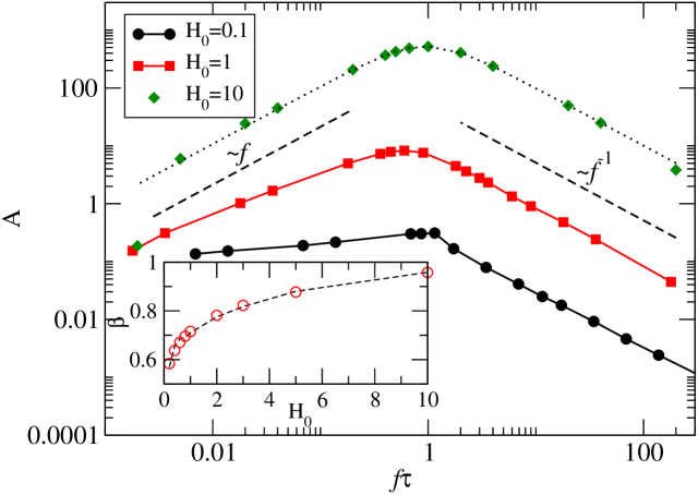
Figure 11: The hysteresis loop area $A$ as a function of the scaled field oscillation frequency at different field strengths $H_{0}$. The upper dashed curve is a fit with the Eq. (19). Inset: Exponent $\beta$ for the LF parts of the $A(f)$ curves as a function of the field amplitude $H_{0}$. Other parameters: $\rho=0.04$, $T^{E}=0.3$.

While the behaviour of the high frequency (HF) asymptotes seems to be universal, the variation of the area at low frequencies is governed by power laws with variable exponents. In the literature on ferromagnetic materials, it is common to present the variation of the loop area in the form $(A-A_{0})\propto H_{0}^{\alpha}f^{\beta}T^{-\gamma}$, where $A_{0}$ is the loop area in the static hysteresis huang.z:2005 . In our model, as the system does not show any static hysteresis, i.e. $A_{0}=0$, we can study the scaling of the area $A$ as is.

The exponent $\beta$ can be measured in the LF region at different system settings. The dependence of the exponent on the driving field amplitude $H_{0}$ is shown in the inset in Figure 11. We observe $\beta$ increase from $0.55$ to 0.95 when the field grows from 0.1 to 10. Asymptotically, the exponent is approaching unity at $H_{0}\to\infty$. Similarly, we can study the scaling exponent $\beta$ at different temperatures. Figure 12 shows the $A(f)$ curves at ambient temperatures from $T^{E}=0.1$ to 10. The exponent is growing with temperature from $\beta=0.55$ at $T^{E}=0$ to $\beta=0.93$ at $T^{E}=1$.

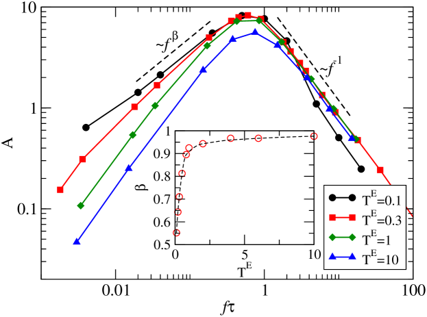
Figure 12: The hysteresis loop area $A$ as a function of frequency $f$ at various temperatures $T^{E}$ ($\rho=0.04$, $H_{0}=1$). Inset: Exponent $\beta$ for the LF parts of the $A(f)$ curves as a function of temperature $T^{E}$.

The sensitivity of the loop area to the field oscillation amplitude is illustrated in Fig. 13. The loop area as a function of the field strength varies according to a power law $A\propto H_{0}^{\alpha}$ with $\alpha$ taking values from 0.9 to 1.9 at $T^{E}$ varying from 0 to 5 (see the inset). Fig. 14 presents a similar scan along the frequency axis. Here we see a qualitative change of the behaviour. Firstly, all the curves show the same asymptotic power law $A\propto H_{0}^{2}$ in sufficiently high fields, $H_{0}>20$. Secondly, in the HF region, at $f\tau>1$, this law is observed at all field strengths. However, the LF behaviour depends on the driving field amplitude. The exponent $\alpha$ grows from 0.75 to 2 in the region $f\tau\leq 1$.

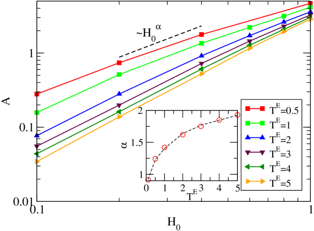
Figure 13: The hysteresis loop area $A$ variation with the field strength $H_{0}$ at various temperatures $T^{E}$ ($\rho=0.04$, $f=0.01$). Inset: Exponent $\alpha$ at different temperatures $T_{E}$.

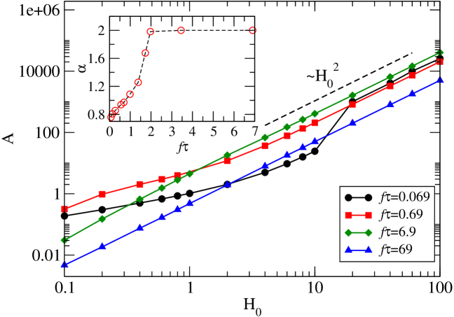
Figure 14: The hysteresis loop area $A$ as a function of the field strength $H_{0}$ at various frequencies $f$ ($\rho=0.04$, $T^{E}=0.3$). Inset: Exponent $\alpha$ as a function of scaled frequency $f\tau$.

Finally, we study the influence of temperature on the loop area in the LF region. The simulation results are shown in Fig. 15 and look intriguing. The loop area grows at low temperatures, then reaches a maximum at about $T^{E}=0.3$ and then shows a power law decay. The areas of the hysteresis loops decrease with the temperature due to the decrease of the alignment and coercivity as temperature is increased. The maximum does not appear at high field amplitudes. The power law exponent at high temperatures, as calculated from a fit with $A\propto(T^{E})^{-\gamma}$, varies from $\gamma=1$ in weak fields to $\gamma\approx 0.3$ in strong fields.

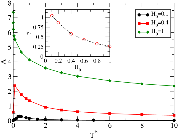
Figure 15: The typical hysteresis loop area $A$ variation with temperature $T^{E}$. Inset: Exponent $\gamma$ as a function of the field strength $H_{0}$. Other parameters: $\rho=0.04$, $f=0.01$.

4 Discussion

The observations for hysteresis in the active swarm agree qualitatively with the corresponding results for 2D magnets huang.z:2005 . First of all, we can note the special role of the orientational relaxation time $\tau$ that determines the timescale for the swarm dynamics. At frequencies lower than $1/\tau$, the active particles have enough time to align with the field and, therefore, the swarm follows the field direction “obediently”. At hight frequencies, $f\tau\gg 1$, the direction of motion of the particles does not change anymore. The action of the field leads just to a minor velocity oscillation about the average value: the motion is slightly slowed down in the opposing field but accelerated if the field is acting in the direction of motion. In this regime, the velocity follows the field direction only half of the time. Finally, at $f\tau\approx 1$, the inability of the swarm to follow the direction of the field is accompanied by the strong variation of the velocity, so that the dynamic coercivity and dynamic remanence are both high, which is reflected in the large loop area.

The variation of the loop shape and area can be understood from the following simple analysis. We consider an ensemble of non-interacting active Brownian particles with energy depot as described by Eqs. (1-2) and calculate an average of the $x$-component of the acceleration over all particles:

$$\left\langle\frac{dV_{ix}}{dt}\right\rangle=\left\langle-\gamma^{E}V_{ix}+\frac{qd}{c+dV_{i}^{2}}V_{ix}+\sqrt{2D^{E}}{\bm{\xi}_{i}}(t)+H_{x}(t)\right\rangle$$ (17)

The averaging eliminates the random term for symmetric noise. If, in addition, we assume a high-dissipation regime such that $c\gg dV_{i}^{2}$, we can rewrite the thrust term as $qd/(c+dV_{i}^{2})\approx qd/c-(qd^{2}/c^{2})V_{i}^{2}$ and arrive to a simple equation for evolution of the order parameter:

$$\frac{d\varphi}{dt}=\left(\frac{qd}{c}-\gamma^{E}\right)\varphi-\frac{qd^{2}}{c^{2}}\left\langle V_{i}^{2}V_{ix}\right\rangle+H_{0}\sin(\omega t)$$ (18)

Averaging of the second term on the right-hand side is not straightforward but we can assume that the term scales approximately as $\varphi^{3}$ romensky.m:2014 if the motion is mostly along the $x$-axis. The depot mode predicts that in absence of field and fluctuations the mean particle velocity is given by Eq. (5). Then, in weak fields and for isotropic motion, the particle speed becomes independent of the direction, so $\langle V_{i}^{2}V_{ix}\rangle\approx V_{0}^{2}\varphi$.

In certain limiting cases we can derive explicit asymptotes for $A(f)$ goldsztein.gh:1997 . The solution can easily be found for the case when the right-hand side of Eq. (18) contains only linear term in $\varphi$ and can be written as $\lambda\varphi+H_{0}\sin(\omega t)$. For passive Brownian particles ($q=0$) in a viscous medium, the second term in Eq. (18) disappears while the first one is simply $-\gamma^{E}\varphi$. Moreover, the function takes the same form for an ABP-DI system in the strong field limit, $H_{0}\gg q/V_{0}$, with $\lambda=\gamma^{E}-dq/c$ playing a role of effective friction coefficient. In this case, the closed form for the whole $A(f)$ curve is described by goldsztein.gh:1997 :

$$A(f)=\frac{1}{2}\frac{H_{0}^{2}f}{\left(\frac{\lambda}{2\pi}\right)^{2}+f^{2}}.$$ (19)

More generally, at high frequencies, $f\tau\gg 1$, the time derivative of $\varphi$ in Eq. (18) becomes very large, so $\frac{d\varphi}{dt}\approx H_{0}\sin{\omega t}$ and a single integration gives $\varphi\propto-\frac{1}{\omega}\cos{(\omega t)}$. Therefore, we find a general high frequency asymptotic result: $A(f)\approx H_{0}^{2}/2f$. In the strong field limit, $H_{0}\gg q/V_{0}$, the steady state speed of the particle is given by $\varphi=\langle V_{ix}\rangle=H_{0}/\gamma^{E}$ and the loop area scales as $A\propto H_{0}^{2}$ as predicted by Eq. (19). Thus, the asymptotic behaviour of $A(f)$ at $H_{0}V_{0}/q\gg 1$ and $f\tau\gg 1$ does not depend on whether the particles are active or passive nor on interactions between them. We can summarise the limiting scaling laws as follows:

• $A\propto f$ ($\beta=1$) at $f\tau\ll 1$ for passive Brownian particles, for non-interacting active particles ($k_{B}T^{E}\gg D(\gamma^{E})^{3}$), or strong fields $H_{0}\gg q/V_{0}$

• $A\propto f^{-1}$ at $f\tau>1$ for all passive and active Brownian particles

• $A\propto H_{0}^{2}$ ($\alpha=2$) at strong fields $H_{0}\gg q/V_{0}$

We can clearly see these scaling laws in the simulation data presented in Figures 11, 12, 14, 16. The low frequency law $A\propto f$ appears in Figs. 11 and 16; the high frequency one $A\propto f^{-1}$ – in Figs. 11, 12, and 16, and the strong field asymptote $A\propto H_{0}^{2}$ is seen in Fig. 14. The scaling law $A\propto f^{-1}$ at $f\tau\gg 1$ seems to be valid at all field magnitudes, as we predicted above.

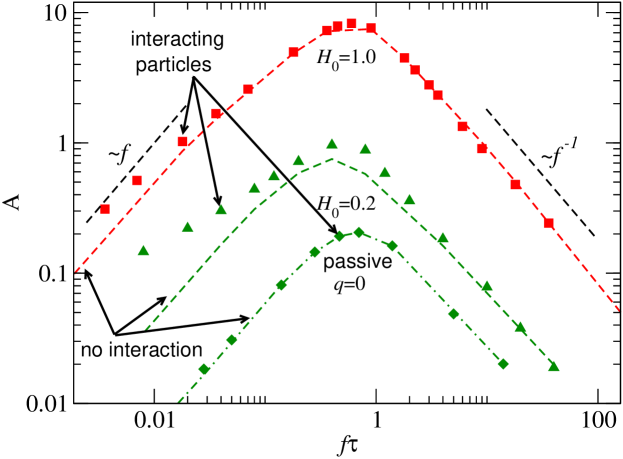
Figure 16: The hysteresis loop area $A$ for an ensemble of passive ($q=0$) and active ($q=1$) Brownian particles at two different field strengths: $H_{0}=0.2$ and $H_{0}=1$. Lines correspond to results obtained with non-interacting agents while symbols denote data for interacting particles. Other parameters: $\rho=0.04$, $T^{E}=0.3$.

Outside the range of these specific simple behaviours, the generic scaling form $(A-A_{0})\propto H_{0}^{\alpha}f^{\beta}T^{-\gamma}$ seems to be valid. However, the exponents for the swarm differ from those for 2D magnets. The observed values of the exponent $\alpha$ (from 0.75 to 2.0) for the swarm are higher than the numbers for the 2D Heisenberg model, where $\alpha=0.40\pm 0.02$ was reported huang.z:2005 . Similarly, the $\gamma$ exponent at high temperatures, $A\propto(T^{E})^{-\gamma}$, taking values from $\gamma=1$ in weak fields to $\gamma\approx 0.3$ in strong fields, is higher than the result 2D Heisenberg model - $\gamma=0.30\pm 0.02$ huang.z:2005 except for the lowest value. The most obvious reason for the difference is the restriction on the order parameter. In the channel confinement, the order parameter becomes one-dimensional. In this sense, the symmetry of our problem is more closely resembling 2D Ising model. Indeed, in the Ising magnet, one finds exponents $\alpha=0.70$, $\beta=0.36$, $\gamma=1.18$ chakrabarti.bk:1999 , which are close to our results at $T^{E}\to 0$, $f\tau\to 0$, and $H_{0}\to 0$, where we have $\alpha=0.75$, $\gamma=1.05$. For the exponent $\beta$, however, we observe values from 0.55 to 0.94, which are higher than $\beta=0.38\pm 0.04$ for Heisenberg ferromagnet and $\beta=0.36$ for Ising ferromagnet chakrabarti.bk:1999 . In our model, the exponent $\beta$ decreases rapidly with the temperature. One can expect that it will reach even lower values for either lower $T^{E}$ or stronger aligning interactions. Beside the exponents, we see a qualitative analogy between the swarms and magnets in other properties. As was found in huang.z:2005 , the peak on the curves $A(T)$ is observed in weak fields and is moving to lower temperatures upon increase of the field oscillation amplitude. In the Heisenberg magnet, however, the peak corresponds to a jump from non-zero loop to zero, such that below the critical temperature the field is unable to reorient the magnetic moment within the oscillation period. Our system seems to allow reorientation at any field value and, therefore, the jump is not observed. The reason for the area decrease at low temperatures is the increased resistance of a fully aligned swarm, which makes the reorientation within the oscillation period harder. The stronger the field, the shorter time it needs to reorient the swarm. That is why we do not see a peak at $H_{0}=1.0$ at the chosen frequency.

Finally, we can comment on the role of interparticle interactions and active propulsion in the observed dynamic hysteresis. These can be illustrated by the data presented in Fig. 16 romensky.m:2014 . For passive Brownian particles, the interactions do not affect the loop area: The areas obtained with or without interactions coincide at all frequencies. For active particles, the loop area is greater than that for passive ones at all frequencies as their speed is generally higher. The difference due to interactions is greatest at low frequencies, $f\tau<1$. The interactions between particles in that region lead to the increase of the loop area, as the motion of interacting active swarm more is persistent than of the non-interactive one. The loop area is hardly affected by interactions at high frequencies, $f\tau>1$ as the particle have no time to develop any collective motion. We should also note that the effect of interactions is most pronounced in weak fields. In strong fields, the differences between the interacting and non-interacting particles as well as between the passive and active ones are small. Thus, a study of the low frequency response and especially exponents $\alpha$ and $\beta$, which are both always lower for the interacting systems, can provide information about the degree of collectivity and order in the motion of an active swarm.

5 Conclusions

We studied the dynamics of active swarms using method and ideas from condensed matter physics. We demonstrated that the swarms in an external field exhibit a dynamic hysteresis, which is qualitatively identical to that observed in magnetics. We measured the hysteresis loops for swarms of simulated active Brownian particles with dissipative interactions at various field oscillation frequencies. Our calculations show that the swarm reaction depends on the ratio of the orientational relaxation time to the field oscillation period. At high field frequencies, the collective component of the behaviour becomes negligible and the swarm behaves as a collection of independent individuals, while at low frequencies the swarm can develop collective dynamics. We derived scaling exponents for several limiting situations of the swarm dynamics: absence of interactions, weak propulsion, strong field, etc. All the limiting laws are confirmed by simulation results for active swarms. For the general case of active interacting particles, the scaling exponents for the hysteresis loop area are non-universal: they depend on the system’s parameters – noise amplitude, interaction strength, and the field amplitude and do not coincide with exponents for 2D lattice models of ferromagnets.

References

- (1) M.A. Krasnosel’skii, A.V. Pokrovskii, Systems with hysteresis (Springer, 1989)
- (2) I.F. Lyuksyutov, T. Nattermann, V. Pokrovsky, Phys. Rev. B 59, 4260 (1999)
- (3) H. Chaté, F. Ginelli, G. Grégoire, F. Raynaud, Phys. Rev. E 77, 046113 (2008)
- (4) I.D. Couzin, J. Krause, R. James, G.D. Ruxton, N.R. Franks, J. Theor. Biol. 218, 1 (2002)
- (5) T. Ihle, Phys. Rev. E 88, 040303 (2013)
- (6) B.K. Chakrabarti, M. Acharyya, Rev. Mod. Phys. 71, 847 (1999)
- (7) P. Reimann, R. Kawai, C. Van den Broeck, P. Hänggi, Europhys. Lett. 45, 545 (1999)
- (8) T. Vicsek, A. Czirók, E. Ben-Jacob, I. Cohen, O. Shochet, Phys. Rev. Lett. 75, 1226 (1995)
- (9) T. Vicsek, A. Zafeiris, Phys. Rep. 517, 71 (2012)
- (10) A. Czirók, A.L. Barabasi, T. Vicsek, Phys. Rev. Lett. 82, 209 (1999)
- (11) J. Toner, Y. Tu, Phys. Rev. Lett. 75, 4326 (1995)
- (12) J. Toner, Y. Tu, Phys. Rev. E 58, 4828 (1998)
- (13) J. Toner, Y. Tu, S. Ramaswami, Ann. Phys. 318, 170 (2005)
- (14) S. Ramaswamy, Annu. Rev. Condens. Matter Phys. 1, 323 (2010)
- (15) G. Baglietto, E.V. Albano, Phys. Rev. E 78, 21125 (2008)
- (16) M. Romenskyy, V. Lobaskin, Eur. Phys. J. B 86, 91 (2013)
- (17) A. Cavagna, A. Cimarelli, I. Giardina, G. Parisi, R. Santagati, F. Stefanini, M. Viale, Proc. Natl. Acad. Sci. USA 107(26), 11865 (2010)
- (18) A.P. Solon, J. Tailleur, Phys . Rev. Lett. 111, 078101 (2013)
- (19) W. Ebeling, F. Schweitzer, B. Tilch, Biosystems 49, 17 (1999)
- (20) W. Ebeling, U. Erdmann, J. Dunkel, M. Jenssen, J. Stat. Phys. 101, 443 (2000)
- (21) V. Lobaskin, M. Romenskyy, Phys. Rev. E 87, 052135 (2013)
- (22) M. Romensky, D. Scholz, V. Lobaskin, Interface 99, 99 (2014)
- (23) P. Romanczuk, M. Bär, W. Ebeling, B. Lindner, L. Schimansky-Geier, Eur. Phys. J. Special Topics 202, 1 (2012)
- (24) P. Español, Phys. Rev. E 52, 1734 (1995)
- (25) K. Binder, Zeitschrift Phys. B Condens. Matter 43, 119 (1981)
- (26) H. Chaté, F. Ginelli, G. Grégoire, F. Peruani, F. Raynaud, Eur. Phys. J. B 64, 451 (2008)
- (27) L. Verlet, Phys. Rev. 159, 98 (1967)
- (28) M. Romensky, V. Lobaskin, T. Ihle, Phys. Rev. E 90, 063315 (2014)
- (29) I.D. Mayergoyz, Mathematical models of Hysteresis (Spinger Verlag, New York, 1991)
- (30) Z. Huang, F. Zhang, Z. Chen, Y. Du, Eur. Phys. J. B 44, 423 (2005)
- (31) E. Vatansever, U. Akinci, Y. Yüksel, H. Polat, J. Magn. Magn. Mater. 329, 14 (2013)
- (32) G.H. Goldsztein, F. Broner, S.H. Strogatz, SIAM J. Appl. Math. 57, 1163 (1997)