The Fast-Superfast Transition in the Sleeping Lagrange Top

Abstract

The fast-superfast transition is a particular movement of eigenvalues found in [4] when studying the family of sleeping equilibria in the Lagrange top. Although this behaviour of eigenvalues typically suggests a change in stability or a bifurcation, in this case there is no particular change in the qualitative dynamical properties of the system. Using modern methods, based on the singularities of symmetry groups for Hamiltonian systems, we clarify the appearance of this transition.

MSC 2010: 70H05; 70H14; 37J20

1 Introduction

The Lagrange top is one of the most well-known simple mechanical systems with symmetries. It consists of an axisymmetric rigid body with a fixed point moving under the influence of a constant gravitational force. One of the important characteristics of this system is that it has two symmetry groups: the rotations around the axis of gravity and the spin about the axis of symmetry of the top. In fact, the energy and the conserved quantities associated with these symmetries make the Lagrange top a Liouville integrable system (see, e.g., [2]).

A special configuration of the system is the sleeping top, when the top is pointing upwards, so that the axis of gravity and the symmetry axis coincide. This position has non-trivial isotropy, since there is a continuous group of symmetries that leaves this configuration invariant. This fact is ultimately responsible for many of the dynamical properties of a sleeping top. In this work, we focus on this particular configuration, but with all possible angular velocities. These solutions are examples of relative equilibria, motions of the system which evolve within the symmetry direction. Generally speaking, relative equilibria act as organising centres of the dynamics of a Hamiltonian system with symmetries and, therefore, their study gives important information about the qualitative behaviour of the dynamical flow which, typically, is impossible to obtain analytically.

Unlike for generic flows, relative equilibria of Hamiltonian systems can be characterised as critical points of a certain function depending on a parameter. This approach is very useful, because it gives necessary conditions for bifurcations of branches of relative equilibria, based on singularity and critical point theory. Indeed, when the second variation of this parameter dependent function becomes degenerate, a new branch of relative equilibria may bifurcate. Typically, one expects that at the bifurcation point, a transfer of stability will occur from the original to the bifurcating branch. However, in the Lagrange top, due to the existence of continuous isotropy, this is not at all the case. For a large part of the family of sleeping Lagrange tops, every point is a bifurcation point to precessing solutions, without the original branch loosing stability. The possibility of a bifurcation from a stable branch to a branch that is also stable was already pointed out by Cartan [1].

These and other phenomena are well known and have been studied in depth from a geometric perspective in [4], where the stability range of sleeping Lagrange tops and their possible bifurcations are computed and the spectral analysis of the linearised dynamics along the sleeping Lagrange top family is carried out. Assuming an oblate body, i.e., the largest moment of inertia is along the symmetry axis, in [4], a diagram similar to the one showed in Figure 1 is presented.

Figure 1: Eigenvalues of the sleeping top as a function of the angular velocity $\lambda$ in an oblate top

When the angular velocity $\lambda$ is zero, the eigenvalues are a real pair. As $\lambda$ is increased, the eigenvalues form a quadruple and when the angular velocity attains the fast-slow critical value $\tau_{f-s}$, the eigenvalues move onto the imaginary axis and the system becomes stable. This fast-slow transition corresponds to a Hamiltonian-Hopf bifurcation (see [3]). The surprising fact noticed in [4] is that if the angular velocity is further increased, two of the eigenvalues cross at zero moving along the imaginary axis for $\lambda^{2}=\tau_{f-sf}$. This point was called the fast-superfast transition. Usually, such an eigenvalue crossing implies the existence of a bifurcation or a change in stability, but from a dynamical point of view, this fast-superfast point has no special behaviour with respect to nearby points in the sleeping top family. On the other hand, one could argue that since all the points in the stable regime exhibit a bifurcation to the precessing branch, a zero eigenvalue at each point in the stable range is expected. However, only a zero eigenvalue is observed in the linearisation at the fast-superfast transition point.

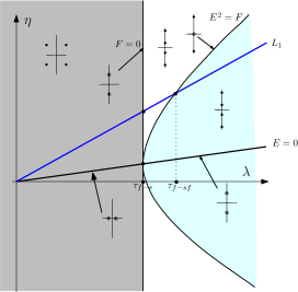
Figure 3: Oblate case

If the body is prolate, i.e., the shortest moment of inertia is along the symmetry axis, the evolution of the eigenvalues is shown in Figure 2. The motions of eigenvalues shown in both figures correspond to those obtained in Figure 3 of [4].

Figure 2: Eigenvalues of the sleeping top as a function of the angular velocity $\lambda$ in prolate top

As in the oblate case, the fast-slow transition is a Hamiltonian-Hopf bifurcation between the stable and unstable regimes, but note that in this case, no fast-superfast transition occurs. It can be shown that the qualitative dynamical behaviour of the system does not depend on the oblateness or prolateness of the body, so the linearisation should not behave differently in the oblate and prolate cases. In particular, the existence of a fast-superfast transition at a unique point in the oblate but not the prolate case, questions our understanding of the qualitative dynamics of the sleeping Lagrange top family.

In this paper, we show that this fast-superfast transition is an artefact due to the existence of continuous isotropy in the sleeping Lagrange top. This has as a consequence that the linearisation done in [3] has implicitly chosen one angular velocity representative among an infinite number of possibilities for the equilibria under study. In fact, we show that for each stable sleeping equilibrium, we can choose the angular velocity in such a way that the linearisation has a double zero eigenvalue crossing and therefore exhibits a fast-superfast transition, for both the oblate and prolate cases.

2 The Setup

The Lagrange top is the symmetric Hamiltonian system defined by the tuple

$$(T^{*}\mathrm{SO}(3),\omega_{c},\mathbb{T}^{2},\mathbf{J},h),$$

where the phase space is the cotangent bundle $T^{*}\mathrm{SO}(3)$ of the proper rotation group $\mathrm{SO}(3)$, equipped with its canonical symplectic form $\omega_{c}$. If we use the identification, given by the right translation

$$\mathcal{P}:=\mathrm{SO}(3)\times\mathbb{R}^{3} \rightarrow T^{*}\mathrm{SO}(3)$$

$$(\Lambda,\pi) \rightarrow (\Lambda,\hat{\pi}\Lambda),\quad\pi\in\mathbb{R}^{3},$$ (1)

then the toral symmetry group $\mathbb{T}^{2}$ acts on on $\mathcal{P}$ as

$$((\theta_{1},\theta_{2}),(\Lambda,\pi))\mapsto(e^{\theta_{1}\widehat{\mathbf{e}_{3}}}\Lambda e^{-\theta_{2}\widehat{\mathbf{e}_{3}}},e^{\theta_{1}\widehat{\mathbf{e}_{3}}}\pi),\quad(\theta_{1},\theta_{2})\in S^{1}\times S^{1}.$$ (2)

The associated canonical momentum map for this action is given by

$$\mathbf{J}(\Lambda,\pi)=(\pi\cdot\mathbf{e}_{3},-\pi\cdot\Lambda\mathbf{e}_{3})\in\mathbb{R}^{2}.$$ (3)

Finally, the Hamiltonian function $h:\mathcal{P}\rightarrow\mathbb{R}$ is

$$h(\Lambda,\pi):=mgl\mathbf{e}_{3}\cdot\Lambda\mathbf{e}_{3}+\frac{1}{2}\pi\cdot\mathbb{I}^{-1}_{\Lambda}\pi,$$

where $\mathbb{I}_{\Lambda}:=\Lambda\mathbb{I}\Lambda^{-1}$ and $\mathbb{I}:=\operatorname{diag}(I_{1},I_{1},I_{3})$ is the inertia tensor of the rigid body in the reference configuration with respect to a principal axes body frame. Notice that, in this reference configuration, the body symmetry axis is $\mathbf{e}_{3}$. Throughout this article we are using both $\mathbb{R}^{3}$ and the space $\mathfrak{so}(3)$ of $3\times 3$ antisymmetric matrices to represent the Lie algebra of $\mathrm{SO}(3)$, identified via the usual Lie algebra isomorphism given by the hat map

$$\hat{\,}:\mathbb{R}^{3} \rightarrow \mathfrak{so}(3)$$

$$\mathbf{x}=(x_{1},x_{2},x_{3}) \mapsto \hat{\mathbf{x}}=\left[\begin{array}[]{ccc}0&-x_{3}&x_{2}\\ x_{3}&0&-x_{1}\\ -x_{2}&x_{1}&0\end{array}\right].$$

In right trivialisation we have $\delta\Lambda=\widehat{\delta\theta}\Lambda\in T_{\Lambda}\mathrm{SO}(3)$. Therefore, a tangent vector $v\in T_{(\Lambda,\pi)}\mathcal{P}$ is represented as $(\delta\theta,\delta\pi)\in\mathbb{R}^{3}\times\mathbb{R}^{3}$.

From this, it is easy to check that the expression for the symplectic form $\omega$ on $\mathcal{P}$ (the pull back of $\omega_{c}$ to $\mathcal{P}$ given by (1)) is given by

$$\omega(\Lambda,\pi)((\delta\theta_{1},\delta\pi_{1})(\delta\theta_{1},\delta\pi_{2}))=\delta\pi_{2}\cdot\delta\theta_{1}-\delta\pi_{1}\cdot\delta\theta_{2}-\pi\cdot(\delta\theta_{1}\times\delta\theta_{2}).$$ (5)

3 The sleeping Lagrange top

In this model, the sleeping Lagrange top is a relative equilibrium at the phase space point $z=(\Lambda,\pi):=(\mathrm{Id},\lambda I_{3}\mathbf{e}_{3})$ with arbitrary velocity $(\xi_{L},\xi_{R})\in\mathbb{R}^{2}=\mathrm{Lie}\,\mathbb{T}^{2}$ satisfying $\xi_{L}-\xi_{R}=\lambda$. This makes the set of all admissible velocities at each relative equilibrium a one-parameter family. In order to see this, and using standard arguments from geometric mechanics (see, e.g., [5], [6]), we have to check that the augmented Hamiltonian

$$h_{(\xi_{L},\xi_{R})}(\Lambda,\pi):=mgl\mathbf{e}_{3}\cdot\Lambda\mathbf{e}_{3}+\frac{1}{2}\pi\cdot\mathbb{I}^{-1}_{\Lambda}\pi-\pi\cdot\mathbf{e}_{3}\xi_{L}+\pi\cdot\Lambda\mathbf{e}_{3}\xi_{R}$$ (6)

has a critical point at $(\mathrm{Id},\lambda I_{3}\mathbf{e}_{3})$. The derivative of $h_{(\xi_{L},\xi_{R})}$ at an arbitrary point $(\Lambda,\pi)\in\mathcal{P}$ is

$$\mathbf{d}h_{(\xi_{L},\xi_{R})}(\Lambda,\pi)(\delta\theta,\delta\pi)=mgl\mathbf{e}_{3}\cdot(\delta\theta\times\Lambda\mathbf{e}_{3})+\delta\pi\cdot\mathbb{I}_{\Lambda}^{-1}\pi+\pi\cdot(\delta\theta\times\mathbb{I}_{\Lambda}^{-1}\pi)-\xi_{L}\delta\pi\cdot\mathbf{e}_{3}+\xi_{R}\delta\pi\cdot\Lambda\mathbf{e}_{3}+\xi_{R}\pi\cdot(\delta\theta\times\Lambda\mathbf{e}_{3})$$

At $(\Lambda,\pi)=(\mathrm{Id},\lambda I_{3}\mathbf{e}_{3})$ this becomes

$$\mathbf{d}h_{(\xi_{L},\xi_{R})}(\mathrm{Id},\lambda I_{3}\mathbf{e}_{3})(\delta\theta,\delta\pi)=(\lambda-(\xi_{L}-\xi_{R}))\delta\pi\cdot\mathbf{e}_{3}$$ (7)

which vanishes precisely when $\xi_{L}-\xi_{R}=\lambda$. Therefore, according to (2), the dynamical evolution of $z=(\mathrm{Id},\lambda I_{3}\mathbf{e}_{3})$ is given by $z(t)=(e^{t\lambda\widehat{\mathbf{e}_{3}}},\lambda I_{3}\mathbf{e}_{3})$.

In order to study the linearisation of the Hamiltonian system at the sleeping equilibrium, we need to compute several more geometric objects. First, from (3), it is clear that

$$\mu:=\mathbf{J}(z)=(\lambda I_{3},-\lambda I_{3}).$$

Second, since $\mathbb{T}^{2}$ is Abelian, the coadjoint stabiliser of $\mu$ is $G_{\mu}=\mathbb{T}^{2}$. Third, from (2), we find that the stabiliser of the phase space point $z=(\mathrm{Id},\lambda I_{3}\mathbf{e}_{3})$ is

$$G_{z}={S^{1}}^{D}:=\{(\theta,\theta)\in\mathbb{T}^{2}\,:\,\theta\in S^{1}\}.$$

A normalised basis for its Lie algebra $\mathfrak{g}_{z}$ is $\frac{1}{\sqrt{2}}(1,1)$, i.e.,

$$\mathfrak{g}_{z}=\mathrm{span}\left\{\frac{1}{\sqrt{2}}(1,1)\right\}.$$

Define $\mathfrak{m}:=\mathrm{span}\left\{\frac{1}{\sqrt{2}}(1,-1)\right\}$ which is a complement to $\mathfrak{g}_{z}$ in $\mathfrak{g}$, i.e.,

$$\mathfrak{g}=\mathfrak{m}\oplus\mathfrak{g}_{z}.$$ (8)

According to this direct sum decompostion, the velocity of the sleeping Lagrange top takes the form

$$(\xi_{L},\xi_{R})=\frac{\lambda}{2}(1,-1)+\eta(1,1),$$ (9)

where $\eta\in\mathbb{R}$ is arbitrary. Since $G_{z}$ is a continuous subgroup of positive dimension, (9) reflects the fact that the velocity of the relative equilibrium $z$, for which the first variation (7) vanishes, is defined only up to an element of $\mathfrak{g}_{z}$. However, its projection $\xi^{\perp}$ onto the subspace $\mathfrak{m}$, according to the splitting (8), sometimes called the orthogonal velocity of the equilibrium, is unique.

4 The Symplectic Slice

The linearisation of the Hamiltonian system at the relative equilibrium $z=(\mathrm{Id},\lambda I_{3}\mathbf{e}_{3})$ is given by

$$L:=\Omega_{N}^{-1}\mathbf{d}^{2}h_{(\xi_{L},\xi_{R})}(\mathrm{Id},\lambda I_{3}\mathbf{e}_{3})\vrule height=12.91663pt,width=0.4pt,depth=6.02773pt\lower 6.02773pt\hbox{\scriptsize$\,N$}\in\mathfrak{sp}(N),$$ (10)

where $(N,\Omega_{N})$ is a symplectic vector subspace of $T_{z}\mathcal{P}$ defined by an arbitrary $G_{z}$-invariant splitting

$$\ker T_{z}\mathbf{J}=T_{z}(G_{\mu}\cdot z)\oplus N,$$

$\Omega_{N}=\omega(z)\vrule height=8.61108pt,width=0.4pt,depth=3.87495pt\lower 3.87495pt\hbox{\scriptsize$\,N$}$, and $\mathbf{d}^{2}h_{(\xi_{L},\xi_{R})}(\mathrm{Id},\lambda I_{3}\mathbf{e}_{3})$ denotes the Hessian of $h_{(\xi_{L},\xi_{R})}$ at the equilibrium point $(\mathrm{Id},\lambda I_{3}\mathbf{e}_{3})$. The vector space $(N,\Omega_{N})$ is often called a symplectic slice.

In order to compute the symplectic slice, we start by studying the fundamental vector fields $(\xi_{1},\xi_{2})_{\mathcal{P}}$ for the action (2), which are given, in the right trivialisation (1), by

$$(\xi_{1},\xi_{2})_{\mathcal{P}}(\Lambda,\pi)=(\xi_{1}\mathbf{e}_{3}-\xi_{2}\Lambda\mathbf{e}_{3},\xi_{1}\mathbf{e}_{3}\times\pi).$$

So, at the sleeping equilibrium $(\text{Id},\lambda I_{3}\mathbf{e}_{3})$, we have

$$T_{(\text{Id},\lambda I_{3}\mathbf{e}_{3})}(G_{\mu}\cdot z)=\mathrm{span}\left\{(\mathbf{e}_{3},0)\right\},$$

where $\mu=\mathbf{J}(z)=(\lambda I_{3},-\lambda I_{3})$ and the coajoint isotropy subgroup is $G_{\mu}=\mathbb{T}^{2}$ (see §3).

Since the derivative of the momentum map is

$$T_{(\Lambda,\pi)}\mathbf{J}(\delta\theta,\delta\pi)=(\delta\pi\cdot\mathbf{e}_{3},-\delta\pi\cdot\Lambda\mathbf{e}_{3}-\pi\cdot(\delta\theta\times\Lambda\mathbf{e}_{3})),$$

at the sleeping Lagrange top point $({\rm Id},\lambda I_{3}\mathbf{e}_{3})$ this becomes

$$T_{(\text{Id},\lambda I_{3}\mathbf{e}_{3})}\mathbf{J}(\delta\theta,\delta\pi)=(\delta\pi\cdot\mathbf{e}_{3},-\delta\pi\cdot\mathbf{e}_{3}-\lambda I_{3}\mathbf{e}_{3}\cdot(\delta\theta\times\mathbf{e}_{3}))$$

and, therefore,

$$\ker T_{(\text{Id},\lambda I_{3}\mathbf{e}_{3})}\mathbf{J}=\{(\delta\theta,\delta\pi)\,:\,\delta\pi\perp\mathbf{e}_{3}\}.$$

Hence, a possible choice for the symplectic slice at $z$ is

$$N=\{(\delta\theta,\delta\pi)\,:\,\delta\theta,\delta\pi\perp\mathbf{e}_{3}\},$$

with symplectic form

$$\Omega_{N}\left((\delta\theta_{1},\delta\pi_{1}),(\delta\theta_{2},\delta\pi_{2})\right)=\delta\pi_{2}\cdot\delta\theta_{1}-\delta\pi_{1}\cdot\delta\theta_{2}-\lambda I_{3}\mathbf{e}_{3}\cdot(\delta\theta_{1}\times\delta\theta_{2}).$$ (11)

It can easily be checked that $N$ is indeed $G_{z}$-invariant and that the isotropy group $G_{z}={S^{1}}^{D}$ acts on $N$ by

$$\varphi\cdot(\delta\theta,\delta\pi)=(e^{{\rm i}\varphi\widehat{\mathbf{e}_{3}}}\delta\theta,e^{{\rm i}\varphi\widehat{\mathbf{e}_{3}}}\delta\pi),\qquad\varphi\in S^{1}\cong{S^{1}}^{D}.$$

5 Stability

In this section, we briefly reproduce the classic stability result for a sleeping equilibrium of the Lagrange top in a formulation adapted to the general framework of this article. This is necessary for the subsequent bifurcation analysis relevant to the fast-superfast transition.

The second variation of the augmented Hamiltonian (6) is

$$\mathbf{d}^{2}h(\xi_{L},\xi_{R})((\delta\theta_{1},\delta\pi_{1}),(\delta\theta_{2},\delta\pi_{2})) = (-mgl-\lambda^{2}I_{3}+\lambda^{2}\frac{I_{3}^{2}}{I_{1}}-\lambda I_{3}\xi_{R})(\delta\theta_{1}\times\mathbf{e}_{3})\cdot(\delta\theta_{2}\times\mathbf{e}_{3})$$

$$+ \left(\lambda\left(1-\frac{I_{3}}{I_{1}}\right)+\xi_{R}\right)\left[\delta\pi_{1}\cdot(\delta\theta_{2}\times\mathbf{e}_{3})+\delta\pi_{2}\cdot(\delta\theta_{1}\times\mathbf{e}_{3})\right]$$

$$+ \delta\pi_{1}\cdot\mathbb{I}^{-1}\delta\pi_{2}.$$

Let

$$\mathbf{u}_{1}=(\mathbf{e}_{1},0),\,\mathbf{u}_{2}=(\mathbf{e}_{2},0),\,\mathbf{u}_{3}=(0,\mathbf{e}_{1}),\,\mathbf{u}_{4}=(0,\mathbf{e}_{2})$$ (12)

be a basis of $N$. Using it and (9), we get $\xi_{R}=\eta-\lambda/2$. Thus, at the sleeping top equilibrium,

$$\mathbf{d}^{2}h_{(\xi_{L},\xi_{R})}(\text{Id},\lambda I_{3}\mathbf{e}_{3})\vrule height=12.91663pt,width=0.4pt,depth=6.02773pt\lower 6.02773pt\hbox{\scriptsize$\,N$}=\begin{bmatrix}A&0&0&B\\ 0&A&-B&0\\ 0&-B&C&0\\ B&0&0&C\end{bmatrix},$$ (13)

where

$$A:=-mgl+\frac{\lambda^{2}I_{3}}{2I_{1}}(2I_{3}-I_{1})-\lambda I_{3}\eta,\quad B:=\frac{\lambda}{2I_{1}}(2I_{3}-I_{1})-\eta,\quad C:=\frac{1}{I_{1}}.$$

The eigenvalues of this matrix are

$$\sigma_{\pm}:=\frac{1}{2}\left((A+C)\pm\sqrt{(A+C)^{2}-4(AC-B^{2})}\right).$$

Thus, $\sigma_{\pm}>0\Longleftrightarrow AC-B^{2}>0$.

Recall from the theory of stability of Hamiltonian relative equilibria (see [7] for a reference appropriate to the isotropy-based approach consistent with this article), that in order to guarantee nonlinear stability it is enough to find an admissible velocity such that (13) is definite. For a sleeping top equilibrium of the form $z=(\text{Id},\lambda I_{3}\mathbf{e}_{3})$, this is equivalent to saying that it is stable if we can find $\eta\in\mathbb{R}$ such that $AC-B^{2}>0$.

Note that

$$AC-B^{2}=-\eta^{2}+\frac{I_{3}-I_{1}}{I_{1}}\lambda\eta+\frac{I_{3}\lambda^{2}}{2I_{1}}-\frac{mgl}{I_{1}}-\frac{\lambda^{2}}{4}.$$

Therefore, for a fixed value of $\lambda$, this is a quadratic function of $\eta$ that attains its maximum value when $\eta$ is equal to

$$\eta^{*}:=\frac{I_{3}-I_{1}}{2I_{1}}\lambda.$$

Substituting this value of $\eta$ in the previous expression yields

$$AC-B^{2}\vrule height=12.91663pt,width=0.4pt,depth=6.02773pt\lower 6.02773pt\hbox{\scriptsize$\,\eta=\eta^{*}$}=\frac{\lambda^{2}I_{3}^{2}-4mglI_{1}}{4I_{1}^{2}}$$

and we conclude that if

$$\lambda^{2}>\frac{4mglI_{1}}{I_{3}^{2}}$$

then the sleeping top equilibrium $(\mathrm{Id},\lambda I_{3}\mathbf{e}_{3})\in\mathcal{P}$ is nonlinearly stable. This is the classical fast top condition. Notice that if

$$\lambda^{2}<\frac{4mglI_{1}}{I_{3}^{2}}$$

then the stability test is inconclusive and this regime must be studied by linearisation methods, as we do in the next section.

6 Linearisation

Formula (11) easily implies that the expressions of the linear symplectic form $\Omega_{N}$ and its inverse, relative to the basis (12), are

$$\Omega_{N}=\begin{bmatrix}0&-\lambda I_{3}&1&0\\ \lambda I_{3}&0&0&1\\ -1&0&0&0\\ 0&-1&&0\end{bmatrix},\qquad\Omega_{N}^{-1}=\begin{bmatrix}0&0&-1&0\\ 0&0&0&-1\\ 1&0&0&-\lambda I_{3}\\ 0&1&\lambda I_{3}&0\end{bmatrix}$$

so the matrix of the linearised system (10) is

$$L=\begin{bmatrix}0&B&-C&0\\ -B&0&0&-C\\ A-\lambda I_{3}B&0&0&B-\lambda I_{3}C\\ 0&A-\lambda I_{3}B&-B+\lambda I_{3}C&0\end{bmatrix}.$$ (14)

The characteristic polynomial of $L$ is

$$t^{4}+\left(2(AC-B^{2})+(2B-CI_{3}\lambda)^{2}\right)t^{2}+(AC-B^{2})^{2},$$

which, after some manipulations, can be written as

$$t^{4}+\frac{E^{2}+F}{2I_{1}^{2}}t^{2}+\frac{(E^{2}-F)^{2}}{16I_{1}^{4}},$$

where

$$E:=I_{3}\lambda-I_{1}(2\eta+\lambda),\qquad F:=I_{3}^{2}\lambda^{2}-4mglI_{1}.$$

Thus, the eigenvalues of $L$ are

$$\varrho_{\pm,\pm}:=\frac{i}{2I_{1}}(\pm E\pm\sqrt{F}).$$ (15)

Notice that for any $\lambda$, that is, for any sleeping top equilibrium, an admissible velocity (equivalently, a value of $\eta$) can be chosen so that $E$ takes any real value. Also, $F$ is positive if and only if $\lambda$ corresponds to an equilibrium for which there is an $\eta$ making the matrix (13) definite. Therefore, we conclude that:

• For any $\lambda^{2}<\frac{4mglI_{1}}{I_{3}^{2}}$, the eigenvalues of the linearisation have non-zero real part and therefore the sleeping equilibrium is unstable. $E$ can be chosen so that the imaginary part is zero (real double pair) or non-zero (complex quadruple) at each point of the unstable regime.

• For any $\lambda^{2}>\frac{4mglI_{1}}{I_{3}^{2}}$, the eigenvalues of the linearisation are purely imaginary. At each point of the stable range, $E$ can be chosen so that we have 4 distinct non-zero eigenvalues, two double imaginary non-zero eigenvalues, or an imaginary pair and a double zero.

Notice that the last property guarantees the existence of one imaginary pair plus a doble zero of the linearised system at each point of the stable range, provided a suitable admissible velocity at that point is chosen. This shows that the fast-superfast transition actually happens at each point of the stable regime if we use the freedom in the isotropy Lie algebra when linearising the system at a sleeping equilibrium.

We now study the relationship between our approach and the results in [4]. First, we notice that in order to obtain a zero crossing of eigenvalues along the sleeping top equilibrium family (the fast-superfast transition) the condition to be satisfied is

$$E^{2}=F,$$

which is equivalent to

$$(2I_{3}-I_{1})\lambda^{2}+4(I_{3}-I_{1})\eta\lambda-4I_{1}\eta^{2}-4mgl=0.$$ (16)

Notice that the moments of inertia inequalities $I_{i}<I_{j}+I_{k}$ for any distinct $i,j,k$, imply that this quadric is a hyperbola in the $(\lambda,\eta)$-plane for any choice of inertia tensor. As we have seen before, one can choose $\eta$ such that $(\lambda,\eta)$ lies on the hyperbola given by (16) if and only if $F>0$ (stable sleeping equilibrium), which holds for both the prolate and oblate cases, as opposed to was observed in [4].

A reason for this apparent disagreement is the following. The approach taken in [4], and based on reduction of the right $S^{1}$-action, corresponds, in our setup, to making the permanent choice $\eta=\lambda/2$ along the family of sleeping equilibria. Therefore, in [4], along this family,

$$(\xi_{L},\xi_{R})=(\lambda,0).$$

Using this choice of velocities, we conclude that (16) is equivalent to

$$\lambda^{2}=\frac{mgl}{I_{3}-I_{1}},$$ (17)

which corresponds, in the axisymmetric case $I_{1}=I_{2}$, to the fast-superfast conditions $(4.24)$ of [4]. Notice that, in the $(\lambda,\eta)$-plane, for a prolate top $I_{3}<I_{1}$, the line $\eta=\lambda/2$ never meets the hyperbola (16). However, for an oblate top $I_{3}>I_{1}$, the fast-superfast transition is found at the unique point (17), which is the intersection of this line with the hyperbola. Both observations are in total agreement with [4].

These considerations are illustrated in the following figures. In Figure 4, the different possibilities for the eigenvalues of the linearised system are shown in the oblate case. The line $L_{1}$, corresponding to the choice $\eta=\lambda/2$ of [4], intersects the hyperbola $E^{2}=F$ precisely at the value $\lambda=\tau_{f-sf}$. Notice, however, that it is possible to find a different relationship between $\lambda$ and $\eta$ such that this intersection happens at any value of $\lambda$ greater than $\tau_{f-s}$, that is, the fast-superfast transition happens at each point of the stable regime in the family of sleeping equilibria for oblate tops.

In Figure 4 the analogous situation for prolate tops is presented. Notice that in this case, the line $L_{1}$ corresponding to the velocity choice in [4] does not intersect the hyperbola $E^{2}=F$. However, as is apparenr from the figure, and exactly as for the oblate case, a different linear relationship between $\lambda$ and $\eta$ can be chosen so that this intersection exists for any value of $\lambda$ in the stable regime.

In both figures we have shown the linear relationship between $\lambda$ and $\eta$ corresponding to the condition $E=0$. Along that line, the eigenvalues of the linearisation always come in pairs; the fast-superfast and the fast-slow transitions occur at the same point.

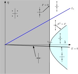
Figure 4: Prolate case

7 Conclusion

The existence of continuous isotropy, and therefore an isotropy Lie algebra $\mathfrak{g}_{z}$ of positive dimension, at a relative equilibrium reflects the fact that the linearisation of the Hamiltonian vector field at the equilibrium, given by (10), is not uniquely defined. The effect of this is that the set of all linearised vector fields should be considered in order to avoid missing pieces of information about the qualitative properties of the Hamiltonian flow near the equilibrium point. In the case of the sleeping Lagrange top, we have shown that the systematic study of the $\mathfrak{g}_{z}$-parametrised family of linearisations given by (14) guarantees that the fast-superfast transition occurs for both prolate and oblate Lagrange tops. Furthermore, in both cases, this transition can be observed for all points in the stable range along the family of sleeping equilibria.

It can be shown that the fast-superfast transitions are closely related to the bifurcations from sleeping to precessing relative equilibria, which are known to happen precisely at each point of the stable range of sleeping tops. This will be studied in detail in [8].

Acknowledgements.

M. R.-O. and M. T.-R. acknowledge the financial support of the Ministerio de Ciencia e Innovación (Spain), project MTM2011-22585 and AGAUR, project 2009 SGR:1338. M. T.-R. thanks for the support of a FI-Agaur Ph.D. Fellowship. M. R.-O. was partially supported by the EU-ERG grant “SILGA”. T. S. R. was partially supported by NCCR SWISSMap and grant 200021-140238, both of the Swiss National Science Foundation.

References

- [1] E. Cartan. Sur la stabilité ordinarie des ellipsoïdes de Jacobi. Proceedings of the International Mathematical Congress, Toronto 1924, volume 2, pages 9–17. The University of Toronto Press, 1928.
- [2] R. Cushman and L. Bates. Global Aspects of Classical Integrable Systems. Birkhäuser Basel, 2004.
- [3] R. Cushman and J.-C. van der Meer. The Hamiltonian Hopf bifurcation in the Lagrange top. In Géométrie symplectique et mécanique (La Grande Motte, 1988), volume 1416 of Lecture Notes in Math., pages 26–38. Springer, Berlin, 1990.
- [4] D. Lewis, T. Ratiu, J. Simo, and J. E. Marsden. The heavy top: a geometric treatment. Nonlinearity, 5(1):1–48, 1992.
- [5] J. E. Marsden. Lectures on Mechanics. Lecture Note Series 174, LMS, Cambridge University Press, 1992.
- [6] J. E. Marsden and T. S. Ratiu. Introduction to Mechanics and Symmetry, second edition. Texts in Applied Mathematics, 17, Springer-Verlag, 1999.
- [7] J. Montaldi and M. Rodríguez-Olmos. On the stability of Hamiltonian relative equilibria with non-trivial isotropy. Nonlinearity 24(10):2777–2783, 2011.
- [8] J. Montaldi and M. Rodríguez-Olmos. Hamiltonian relative equilibria with continuous isotropy. In preparation.
- [9] J.-P. Ortega and T. S. Ratiu. Stability of Hamiltonian relative equilibria. Nonlinearity, 12(3):693–720, 1999.