Reflection nebulae in the Galactic Center: the case for soft X-ray imaging polarimetry

Abstract

Context. Despite numerous attempts with spectroscopic and timing analyses, the origin of irradiation and fluorescence of the 6.4 keV bright giant molecular clouds surrounding Sgr A^∗, the central supermassive black hole of our Galaxy, remains enigmatic.

Aims. Testing the theory of a past active period of Sgr A^∗ requires to open a new observational window: X-ray polarimetry. In this paper, we aim to show how modern imaging polarimeters could revolutionize our understanding of the Galactic Center.

Methods. Through Monte Carlo modeling, we produce a 4 – 8 keV polarization map of the Galactic Center, focusing on the polarimetric signature produced by Sgr B1, Sgr B2, G0.11-0.11, Bridge E, Bridge D, Bridge B2, MC2, MC1, Sgr C3, Sgr C2, and Sgr C1. We estimate the resulting polarization arising from those scattering targets, include polarized flux dilution by the diffuse plasma emission detected toward the GC, and simulate the polarization map that modern polarimetric detectors would obtain assuming the performances of a mission prototype.

Results. The eleven reflection nebulae investigated in this paper present a variety of polarization signatures, ranging from nearly unpolarized to highly polarized ($\sim$ 77%) fluxes. Their polarization position angle is found to be normal to the scattering plane, as expected from previous studies. A major improvement in our simulation is the addition of a diffuse, unpolarized plasma emission that strongly impacts soft X-ray polarized fluxes. The dilution factor is in the range 50% – 70%, making the observation of the Bridge structure unlikely even in the context of modern polarimetry. The best targets are the Sgr B and Sgr C complexes, and the G0.11-0.11 cloud, arranged in the order of decreasing detectability.

Conclusions. An exploratory observation of a few hundred kilo-seconds of the Sgr B complex would allow a significant detection of the polarization and be sufficient to derive hints on the primary source of radiation. A more ambitious program (few Ms) of mapping the giant molecular clouds could then be carried out to probe with great precision the turbulent history of Sgr A^∗, and place important constraints on the composition and three-dimensional position of the surrounding gas.

1 Introduction

Using the Herschel satellite, Molinari et al. (2011) recently discovered a massive ($\sim$ 3$\times$10⁷ M_⊙), continuous chain of irregular, cold dusty clumps in the vicinity of Sgr A^∗, the central supermassive black hole (SMBH) of the Milky Way. The thermal, far-infrared images obtained reveal a $\infty$-shaped, twisted ring that is reminiscent of the persistent dusty tori surrounding the central regions of active galactic nuclei (AGN). In addition, the geometrical size of the circumnuclear gas structure, its column density in excess of 10²⁴ cm^-2, and its orbital speed ($\sim$100 km.s^-1, Molinari et al. 2011), are compatible with AGN tori (Shi et al., 2006). Yet, the current quiescent X-ray luminosity of Sgr A^∗ ($L_{X}\leavevmode\nobreak\ \sim$ 2 $\times$ 10³³ ergs.s^-1, Baganoff et al. 2001) is orders of magnitude lower than what is observed in Seyfert-1 AGN ($L_{X}\leavevmode\nobreak\ >$ 10⁴⁰ ergs.s^-1), where high accretion rates (typically 0.01 to 0.2 M_⊙.y^-1, Meyer et al. 2011) provide efficient radiating engines. Therefore, the question of a more turbulent history, i.e. an active phase, of Sgr A^∗ becomes of prime interest.

It has been suggested that the central SMBH underwent at least two high-luminosity periods, bright enough to illuminate its environment (Inui et al., 2009; Ponti et al., 2010). Traces of this potential activity can be found from the epoch of Granat, when Sunyaev et al. (1993) provided broadband 15’ resolution images of the Galactic Center (GC). In their observations, the GC is characterized by a spherical shape in the 2.5 – 5 keV X-ray band and by an extended (i.e. elongated along the Galactic plane) morphology in the 8.5 – 19 keV energy range. To explain such a difference in the spatial structure of the GC emission, Sunyaev et al. (1993) suggested that part of the diffuse emission of the molecular gas clouds, associated with very steep spectra and strong iron fluorescent emission lines (Koyama et al., 1996), may be due to Compton scattering of photons originating from a nearby compact source. Additional detections of hard X-ray spectral slopes and Fe K$\alpha$ emission lines from a variety of neighboring GC gas clouds (Murakami et al., 2001b; Ponti et al., 2010; Capelli et al., 2012) strengthened the classification of a tenth of giant molecular clouds as reflection nebulae, echoing past Sgr A^∗ outbursts.

The spatial position of the reflectors becomes crucial in the process of determining the goodness of the flaring theory (with estimated $L_{X}>$ 10³⁹ erg.s^-1). Churazov et al. (2002) proved that a polarimetric mission, inherently sensitive to the morphology and the location of reprocessing targets, is the most adequate solution to investigate the re-emitted flux of the scattering molecular clouds. In their model, the Sgr B2 cloud is expected to produce a high polarization degree associated with a direction of polarization normal to the scattering plane. A more elaborate investigation has been undertaken in Marin et al. (2014), where we produced 8 – 35 keV polarization maps of the GC. We avoided the soft X-ray energies, since past X-ray observations (Koyama et al., 1986, 1989; Sidoli & Mereghetti, 1999) have revealed the presence of a diffuse plasma emission angularly superimposed to the X-ray emission of the molecular clouds. This diffuse emission can be well-explained with a two-temperature plasma with T${}_{\rm 1}\leq$ 1 keV and T₂ = 5 – 7 keV (Koyama et al., 2007). It is probably due to a multitude of faint sources (accreting white dwarfs and coronally active stars, Revnivtsev et al. 2009). This X-ray component should be basically unpolarized (Mewe, 1999), ultimately diluting the polarization signal at energies $E$ below 7 keV. Avoiding those energies in Marin et al. (2014), we conservatively modeled the Sgr B2 cloud following the prescription by Churazov et al. (2002). We also implemented a simple structure for the Sgr C complex, as well as the dusty, twisted ring discovered by Molinari et al. (2011), and a reservoir of gas surrounding the inner 5 pc around Sgr A^∗ (not to be mistaken for an accretion disk). It was found that only the two reflection nebulae can be detected at high energies, but it is unknown if similar results hold at $E\leavevmode\nobreak\ \leq$ 7 keV.

It is the scope of this paper to extend the investigation of Churazov et al. (2002) and Marin et al. (2014) to the soft X-ray band, by increasing the number of reflection nebulae in the model, and estimating the plasma and the reflected contributions for the molecular clouds in order to produce a realistic, 4 – 8 keV polarization map of the GC. In a crowded field such as the GC, the presence of an imaging detector becomes necessary to resolve the faint gas clouds and probe the scattering pattern of radiation. To precisely localize the reflection nebulae, characterize their composition and reveal the past activity of Sgr A^∗, we present in Sect. 2.1 the Monte Carlo simulations we performed to obtain a synthetic polarimetric image of the GC. We estimate the polarized flux dilution by the diffuse plasma emission detected toward Sgr A^∗ and compute the diluted polarization signal that a modern imaging polarimeter could detect from space in Sect. 2.2. We discuss our results and conclude our paper in Sect. 3.

2 A polarimetric, soft X-ray, view of the Galactic Center

2.1 Modeling the polarization from reflection nebulae

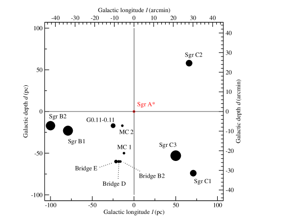
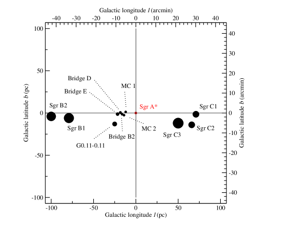
Figure 1: Sketch of the GC model as seen from two directions. Top: view from the direction of the Galactic pole; the Earth is situated toward negative Galactic depths. Bottom: view from Earth; each cloud is projected on the plane of the sky (the Galactic plane).

Molecular cloud	Cloud radius (pc)	Projected distancea (pc)	Line of sight distanceb (pc)	Offsetc (pc)	Velocityd (km.s-1)	Hydrogen column density ($\times$ 1022 cm-2)	Electron optical depth	References
Sgr B2	5	-100	-17	-4.0	60	80	0.5	E,I
Sgr B1	6	-79.1	-23	-6	-45	12.3	0.3	A,D,G
G0.11-0.11	3.7	-25	-17	-13	25	2	0.03	E,F
Bridge E	2.0	-21.6	-60	-1.3	55	9.6	0.07	B,E,F
Bridge D	1.6	-18.3	-60	0.5	55	13.2	0.09	B,E,F
Bridge B2	1.8	-16.3	-60	-1.5	55	12.3	0.08	B,E,F
MC2	1.8	-14	$<$-17	-2.6	-10	$<$2	0.36	C,E
MC1	1.8	-12	-50	1.3	-15	4	0.32	E
Sgr C3	6	50	-53	-12	60	8.7	$<$1	H,E
Sgr C2	4.7	66	58	-14	60	11.4	$<$1	H,E
Sgr C1	4.7	71	-74	-1.5	60	6.5	$<$1	H,E

Table 1: Parameterization of the reflection nebulae, modeled with uniform-density, spherical clouds filled with cold, solar abundance matter. ^aPositive = East of the Galactic center; ^bPositive = behind the Galactic plane (farther to us than Sgr A^∗); ^cPositive = above the equatorial plane. ^dPositive = away from Earth. References – A: An et al. (2013); B: Capelli et al. (2012); C: Clavel et al. (2013); D: Downes et al. (1980); E: Ponti et al. (2010); F: Ponti et al. (2014); G: Ryu et al. (2009); H: Ryu et al. (2013) and I: Sunyaev et al. (1993).

We model the past activity of Sgr A^∗ as a point-like accreting source at the location of the SMBH, emitting an unpolarized spectrum with a spectral energy distribution $F_{\rm*}\leavevmode\nobreak\ \propto\leavevmode\nobreak\ \nu^{-\alpha}$ ($\alpha=1.0$, Porquet et al. 2003, 2008; Nowak et al. 2012). The resulting 4 – 8 keV emission is isotropic and photons journey through the model until absorption/reemission/scattering onto the giant molecular gas clouds. Polarization of the observed signal then arises from Compton scattering of the reprocessed light, where the scattering angle determines the polarization degree and the polarization angle of the intercepted signal that can be recorded at the detector. The reflection nebulae are modeled with uniform-density, spherical clumps filled with neutral solar abundance matter and located according to the most recent constraints from infrared-to-X-rays observations (see Tab. 1). A sketch of the model is presented in Fig. 1, showing the location of the reflection nebulae from a polar view (top figure) and on the plane of the sky (i.e. the Galactic plane, bottom figure). The axes are labeled in parsecs and arcminutes.

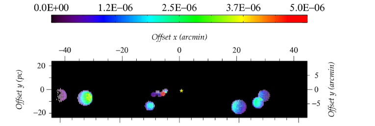
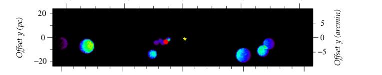
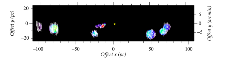
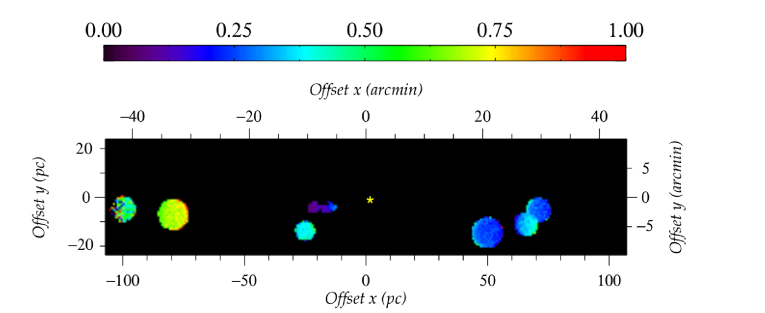
Figure 2: Simulated model images of the $\sim$ 100 pc $\times$ 20 pc region around Sgr A^∗. The top map shows the combination of polarized flux, $PF/F_{\rm*}$ (color-coded, with the color scale shown on top of the image in arbitrary units), polarization position angle $\psi$ (white bars drawn in the center of each spatial bin), and polarization degree $P$, whose value is proportional to the length of the bars. The second map is the polarized flux only, the third image the polarization position angle $\psi$ with artificially extended white vectors for better visibility, and the bottom map represents the $P$, color-coded, with the color scale shown on top of the image in fraction of polarization. A yellow star indicates the position of Sgr A^∗.

Three-dimensional radiative transfer is achieved using stokes (Goosmann & Gaskell, 2007; Marin et al., 2012), a Monte Carlo code that includes a coherent treatment of polarization, multiple scattering, and an imaging routine. Computation of the re-emitted spectra includes algorithms for inelastic Compton scattering onto bound electrons, photo-absorption and iron line fluorescent. The emission direction, the distance that photons travel between reprocessing events, and the scattering angles are computed by Monte Carlo routines based on classical intensity distributions. Mueller matrices are used to evaluate the change in polarization after each scattering event. Photo-absorption above the atom K-shell and the subsequent emission of K$\alpha$ and/or K$\beta$ line photons is included and weighted against the probability of Auger effects. For further details about the code, please refer to the complete description of the polarization properties and transformation of radiation during scattering events described in Goosmann & Gaskell (2007), Marin et al. (2012) and Marin & Dovčiak (2015).

We sample a total of 7$\times$10¹¹ photons in a model with a spatial resolution set to 270$\times$270 bins for the longitudinal and latitudinal offsets, so that the photon flux is divided into 72900 pixels. Each of these pixels is labeled by its position offset in parsecs and arcminutes, and stores the four Stokes parameters of the photons. The spatial resolution is equal to 0.8 pc, which represents 20 arcsecs at the distance of the GC (8.5 kpc, Ghez et al. 2008). Finally, the model space is divided in 20 polar and 10 azimuthal viewing directions. Note that due to the three-dimensional meshes of the coordinate grid, the shape of the scattering regions is slightly deformed in the image projection process.

The resulting polarization maps of the GC, integrated over the whole 4 – 8 keV band to maximize detection, are presented in Fig. 2. The top figure shows a triple combination of 1) the polarized flux ($PF/F_{\rm*}$, i.e. intensity $\times$ polarization degree), color-coded and displayed with arbitrary units, 2) the polarization degree $P$, and 3) the polarization position angle $\psi$ identified by white bars drawn in the center of each spatial bin. A vertical bar indicates a polarization angle of $\psi$ = 90^∘ and a horizontal bar stands for an angle of $\psi$ = 0^∘. The length of the bar is proportional to $P$. The second figure shows the polarized flux only and the third is a visual representation of $\psi$ with artificially extended white vectors for better visibility. The fourth, bottom, map depicts the polarization degree with its own color code, ranging from 0 (unpolarized) to 1 (fully polarized).

From East to West, we find that Sgr B2 presents a high polarization degree (65.0 %) associated with very small polarized fluxes (a consequence of its large hydrogen column density and distance from the irradiating source). The polarized flux map (Fig. 2, top) clearly shows a brightness distribution of the flux on the contours of the molecular gas model that is facing the SMBH, such as observed by Murakami et al. (2001a). Sgr B1 has the highest polarization degree of the GC, up to 76.9 %. Its size and location allow a large polarized flux to be observed. Similarly to the other big structures, the re-emission pattern from the cloud can be probed in great detail by imaging polarimeters. Similarly, G0.11-0.11 shows large polarized fluxes due to a reasonably high $P$ (55.8 %). The Bridge globally displays medium-to-low polarized fluxes. The three-dimensional location of the clouds forming the Bridge (Bridge D, Bridge E, Bridge B2, MC1 and MC2) explains their lower polarization degrees (from 0.06 to 15 %) in comparison with the other scattering nebulae (see Fig. 1). One notable exception is the MC2 cloud, exhibiting a polarization degree up to 25.8 % since, being the closest cloud to Sgr A^∗, its scattering angle with respect to the source and the observer is more favorable. The $\sim$ 10 % polarization of MC2’s neighboring, coplanar clouds (Bridge B2 and E) arises from scattering of high-$P$ photons reprocessed on MC2 and then reaching the observer. Finally the Sgr C complex behaves uniformly despite the dispersion of its three clouds with respect to the line-of-sight distance. They exhibit moderate polarized fluxes and polarization degrees of the order of 32 %. All the clouds display a polarization position angle $\psi$ normal to the scattering plane (i.e. close to 90^∘). We summarize the integrated $P$ and $\psi$ in the first two columns of Tab. 2.

Thus, the GC presents a large panel of polarization signatures associated with polarization degrees varying from high (76.9 %) to very low values (0.1 %). The blend of the polarization signals originating from the Sgr B and Sgr C complexes, and from the Bridge structure, underlines the need for an imaging detector with a sufficient spatial resolution in order to resolve structures as small as the Bridge clouds. Additionally, our results are found to be consistent with the pioneering simulation of Churazov et al. (2002) and their higher energy counterpart (Marin et al., 2014). However, in the light of our previous (8 – 35 keV) simulations (Marin et al., 2014), it is worth mentioning that our polarization results strongly depend on the real location of the reflection nebulae. As it was shown in the aforementioned article, the degree of polarization resulting from reprocessing onto the outer layers of the cloud approximately varies as the square of the cosine of the scattering angle between the source, the cloud, and the observer’s position. With new estimations of the true location of the scattering nebulae, first order corrections can be then applied to results from Tab. 2 (see, e.g., discussion in Kruijssen et al. 2014, 2015).

2.2 Polarization dilution by the GC diffuse plasma emission and detectability with modern instruments

Molecular cloud	P (%)	$\psi$ (∘)	$f_{\mathrm{R}}$ (%)	Pexp. (%)	Pdetect. (%)	$\psi_{\rm detect.}$ (∘)
Sgr B2	65.0	88.3	70.0	45.5	57.4$\leavevmode\nobreak\ \pm\leavevmode\nobreak\$4.4	83.3$\leavevmode\nobreak\ \pm\leavevmode\nobreak\$3.4
Sgr B1	76.9	84.4	52.6	40.5	40.4$\leavevmode\nobreak\ \pm\leavevmode\nobreak\$3.9	80.3$\leavevmode\nobreak\ \pm\leavevmode\nobreak\$3.3
G0.11-0.11	55.8	61.6	–	–	–	–
Bridge E	12.7	67.9	–	–	–	–
Bridge D	0.1	74.2	–	–	–	–
Bridge B2	15.8	77.8	–	–	–	–
MC2	25.8	73.8	–	–	–	–
MC1	0.1	77.5	–	–	–	–
Sgr C3	32.9	106.4	50.7	16.7	15.5$\leavevmode\nobreak\ \pm\leavevmode\nobreak\$2.4	109.0$\leavevmode\nobreak\ \pm\leavevmode\nobreak\$4.5
Sgr C2	34.9	99.1	63.0	22.0	17.9$\leavevmode\nobreak\ \pm\leavevmode\nobreak\$3.8	99.1$\leavevmode\nobreak\ \pm\leavevmode\nobreak\$5.6
Sgr C1	31.1	94.6	60.2	18.7	23.1$\leavevmode\nobreak\ \pm\leavevmode\nobreak\$3.3	98.1$\leavevmode\nobreak\ \pm\leavevmode\nobreak\$6.0

Table 2: Integrated 4 – 8 keV polarization degree $P$ of the reflection component (including neutral iron lines) and polarization position angle $\psi$ of the GC molecular clouds from the simulation with stokes. Polarization angles are defined with respect to Galactic North, with positive defined as West to North. The fraction of the total flux that is reflected $f_{\mathrm{R}}$ is computed from Ryu et al. (2009) and Ryu et al. (2013), allowing us to evaluate the diluted polarization signal P_exp.. Using Monte Carlo simulations associated with the GPD instrument (see text), we finally show estimations of the polarization degree P_detect. and angle $\psi_{\rm detect.}$ that a future polarimeter would detect. The empty cells correspond to clouds with too low X-ray luminosities to be observed within 3 Ms or with unestimated fractions of the reflected flux.

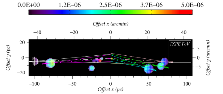
Figure 3: Integrated polarization image of the GC showing how the angle of polarization would constrain the position of the illuminating source. The polarized flux is shown, color-coded and with arbitrary units. The field of view (FoV) of our test case IXPE is indicated with a white box, and a yellow star indicates the position of Sgr A^∗. Colored segments (Sgr B2: white; Sgr B1: magenta; Sgr C3: cyan; Sgr C2: green; Sgr C1: pink) are representative of the estimated polarization position angle (dashed line) and its associated error (solid line).

To evaluate how modern imaging polarimeters may constrain the angular position of the source which illuminated the GC molecular clouds in the past, we simulate their observations taking into account the complex environment in which these sources are immersed. One of the most elaborate, technologically-ready X-ray polarimeter is the Gas Pixel Detector (GPD, Costa et al. 2001; Bellazzini et al. 2006; Bellazzini & Muleri 2010). The GPD is particularly sensitive to the X-ray polarization in the 2 – 10 keV energy range, also offering fine location accuracy and moderate energy resolution (Muleri et al., 2010; Fabiani et al., 2014). These characteristics are very well matched with the required moderate angular resolution of 4 – 5 arcmin for performing these observations (see Fig. 1).

As a test case of the GPD in the context of modern polarimetric missions, we rely on the imaging capabilities of IXPE (the Imaging X-ray Polarimetry Explorer, a mission concept to be proposed to the next NASA/SMEX call). The IXPE’s 30 arcsec half-power diameter roughly corresponds to the spatial resolution of our images, so that a comparison between the resolution of the instrument and our simulation is straightforward. Equipped with GPDs, such a mission will allow to single out and remove the contribution of any point-like sources, even if transient (namely, Sgr A* flares and transients), which may be active during the observation; therefore we can safely neglect any contamination from those sources. Nonetheless, we have to account for the diffuse Galactic plasma emission that is expected to be unpolarized and in any case not correlated with the position of the illuminating source. Therefore, the plasma contribution has to be subtracted from the flux coming from the molecular cloud; alternatively, the simulated polarization has to be diluted, with respect to the values presented in the previous section, by an amount which depends on what fraction of the total flux is due to the reflected component. While during flight we could always compare the results from these two different methods, in this paper we choose the latter for practical reasons.

We estimate the plasma and the reflected contributions for the molecular clouds in the Sgr B and Sgr C complexes by means of the spectral decomposition performed by Ryu et al. (2009) and Ryu et al. (2013), respectively. In these works, the spectra of Sgr B1, Sgr B2, Sgr C1, Sgr C2 and Sgr C3 are each fitted with two spectral components which separately take into account the plasma contribution and the emission due to the reflection of the external source radiation. Labeling these two spectral components $F_{\mathrm{plasma}}(E)$ and $F_{\mathrm{refl.}}(E)$, the “dilution” factor $f_{\mathrm{R}}$ by which we multiply the polarization presented above to obtain the expected degree polarization $P_{\mathrm{exp.}}$ is:

$$f_{\mathrm{R}}=\frac{\int_{4\leavevmode\nobreak\ \mathrm{keV}}^{8\leavevmode\nobreak\ \mathrm{keV}}F_{\mathrm{refl.}}(E)\mathrm{d}E}{\int_{4\leavevmode\nobreak\ \mathrm{keV}}^{8\leavevmode\nobreak\ \mathrm{keV}}\left[F_{\mathrm{refl.}}(E)+F_{\mathrm{plasma}}(E)\right]\mathrm{d}E},$$ (1)

where $E$ is the energy. The energy interval 4 – 8 keV is chosen to maximize the reflected contribution in the energy range where IXPE is most sensitive. The dilution $f_{\mathrm{R}}$ for the different clouds is in the range 50% – 70% assuming the best fit parameters estimated by Ryu et al. (2009) and Ryu et al. (2013) (see Tab. 2); however, the uncertainty on this value depends on the uncertainties on the parameters of the fit deconvolution. For example, changing such parameters in the 90% confidence level in case of Sgr B2 results in a value of $f_{\mathrm{R}}$ between about 64% and 75%, with a mean value of 70% which coincides with the number reported in Tab. 2. Therefore, there is a systematic uncertainty on the expected polarization of the order of about 10% of its value, but this does not affect our ultimate goal, which is to explore the feasibility of the polarization measurement with reasonable assumptions. Moreover, it is reasonable to assume that when the measurement will be actually done, such a systematic uncertainty will be reduced by the more accurate measurements carried out by other spectroscopy-dedicated satellites.

The inputs for the Monte Carlo routine (described in detail in Dovčiak et al. 2011), are the net polarization $P_{\mathrm{exp.}}$, reported in Tab. 2, and the flux of each molecular cloud. This returns an estimate of the measured polarization for the selected observation time. The GPD field of view is sufficient to observe the Sgr B and Sgr C complexes in a single pointing each; therefore, we assumed to carry out a single 1 Ms long observation for Sgr B and another single 2 Ms long observation of Sgr C, whose expected degree of polarization is lower because of the less favorable scattering geometry. We also estimated the detector’s residual background rate, based on past flown gas detectors with similar gas mixture. Thanks to the GPD’s imaging capabilities, this is about 10 times smaller than the expected signal from the reflected component of the molecular clouds. The results are reported in Tab. 2 and shown graphically in Fig. 3. In this picture, we reported the polarization angles $\psi_{\rm detect.}$ such as they would be measured by a modern imaging polarimeter with a $1\sigma$ error of a few degrees for each cloud. Fig. 3 demonstrates that the measurement of $\psi$ would allow us to constrain the angular position of the illuminating source very tightly. Moreover, the five molecular clouds provide as many independent constraints, so it is clear that a future X-ray polarimetric satellite equipped with a mapping instrument would be able to test unambiguously the scattering origin of the X-ray emission from GC molecular clouds. In principle, all the other mentioned molecular clouds could be observed (e.g. G0.11-0.11, the Bridge, MC1 or MC2) with a single pointing. However, due to their lower expected net polarization, as well as the increased contribution of the plasma emission, the observation strategy for those reflection nebulae will be driven by the results obtained for the Sgr B and the Sgr C complexes.

3 Concluding remarks

To probe the crowded field of the GC, an instrument with imaging capability is essential. X-ray polarimetry is needed to test (in a novel way) the physical processes operating near the Galactic supermassive black hole.

In this paper, we simulated the 4 to 8 keV polarization response of the observed, 6.4 keV bright giant molecular regions in the GC to a Sgr A^∗ flaring event. We found that the scattering nebulae present a variety of polarization signatures, ranging from nearly unpolarized to highly polarized (with $P\sim$ 77%) fluxes. The brightness distribution of the reprocessed flux compared with the contours of the spherical clumps is in agreement with past observations and tends to point towards a flaring scenario to explain the detection of hard X-ray spectra and prominent iron K$\alpha$ fluorescence features. Future observations would be able to test our predictions against an alternative mechanism proposed to explain the same X-ray signatures by low-energy cosmic-ray electron interactions with neutral matter (Valinia et al., 2000; Yusef-Zadeh et al., 2002). This scenario, not specifically excluded by observations (Capelli et al., 2011), suggests that the resulting X-ray power-law originates from thermal bremsstrahlung emission, and thus the net polarization would be either null for an isotropic distribution of electrons, or at least different from Compton scattering-induced polarization. The key feature needed to discriminate between the two scenarios is to measure the angle of polarization. Indeed, in comparison with the observed degree of polarization affected by the Galactic plasma and by its characteristics, the polarization position angle of a photon will not suffer any GC plasma-induced rotation along its journey towards Earth.

To assess the validity of the flaring hypothesis, we simulated an observation of the reflection nebulae with the GPD, a modern imaging polarimeter to be mounted on future X-ray polarimetric satellites, taking into account the presence of a diffuse, unpolarized, plasma emission towards the GC. While such an effect decreases the amount of polarization, we found that with a 1 Ms observation of the Sgr B complex and/or with a 2 Ms observation of the Sgr C complex, the polarization imager of a future instrument would be able to unambiguously determine the history of Sgr A^∗ by pinpointing the source of the primary emission.

In this context, the presence of 7 transient X-ray binaries within 23 pc of the GC (4 within 1 pc, Muno et al. 2005) could be a challenge for future observations since a past X-ray outburst of one of these sources could have mimicked a Sgr A^∗ flare. However, since those objects are likely low-mass X-ray binaries (ibid.), their putative past outburst would hardly exceed 10^37-38 ergs.s^-1 (assuming L_X = 0.1$\dot{M}_{\rm peak}$c², Dubus et al. 2001), which is still two orders of magnitude lower than the expected light echo of Sgr A^∗ ($L_{X}>$ 10³⁹ erg.s^-1). In addition, Fig.3 shows that modern imaging polarimeters are able to constrain the emitting source to within less than 10 pc around the SMBH, removing half of the X-ray transients.