Rank-Two Beamforming and Power Allocation in Multicasting Relay Networks

Abstract

In this paper, we propose a novel single-group multicasting relay beamforming scheme. We assume a source that transmits common messages via multiple amplify-and-forward relays to multiple destinations. To increase the number of degrees of freedom in the beamforming design, the relays process two received signals jointly and transmit the Alamouti space-time block code over two different beams. Furthermore, in contrast to the existing relay multicasting scheme of the literature, we take into account the direct links from the source to the destinations. We aim to maximize the lowest received quality-of-service by choosing the proper relay weights and the ideal distribution of the power resources in the network. To solve the corresponding optimization problem, we propose an iterative algorithm which solves sequences of convex approximations of the original non-convex optimization problem. Simulation results demonstrate significant performance improvements of the proposed methods as compared with the existing relay multicasting scheme of the literature and an algorithm based on the popular semidefinite relaxation technique.

I INTRODUCTION

“Beamforming is a versatile and powerful approach to receive, transmit, or relay signals-of-interest in a spatially selective way in the presence of interference and noise” [1]. Recently, the concept of receive and transmit beamforming has been used to enhance coverage and data rate performance in amplify-and-forward (AF) relay networks. Distributed beamforming has been applied as a coherent transceiver technique in a variety of relay network architectures, such as single-user networks [2]–[6]. In such networks one source transmits data to one destination. Single-user networks have been extended to peer-to-peer networks, where multiple source-destination pairs communicate directly via relays [7], [8], [12]. Moreover, distributed systems of non-connected relays can be used for multicasting to transmit data from one source to many destinations simultaneously to avoid exhaustive individual transmissions [9]–[11].

The task to select the optimum antenna weights in centralized beamforming systems using a connected antenna array [13]–[22], or in distributed beamforming systems using a non-connected array [9]–[11] for multicasting is highly non-trivial as it requires to form beams towards several destinations, each corresponding to a different spatial signature. In [13], it has been shown that the problem of selecting the antenna weights for single-group multicasting is NP-hard. Until now, no polynomial time algorithm for NP-hard problems is known and it is expected that exact solutions can only be computed within exponential time.

To derive adequate solutions to beamforming problems which belong to the class of non-convex quadratically constrained quadratic optimization problems (QCQPs), computationally efficient algorithms have been proposed which approximate the feasible set of the optimization problem [8]–[10], [12]–[19], [22]–[33].

Outer approximation techniques replace the QCQPs by convex semidefinite programs (SDPs) which can be solved efficiently [12]–[19]. In the latter approach, the weight vector is replaced by a positive semidefinite Hermitian matrix. Since this so-called semidefinite relaxation (SDR) technique extends the feasible region, a solution matrix to the SDR problem lies not necessarily in the feasible set of the original problem. If the rank $\mathcal{R}(\mathbf{X}^{\star})$ of the solution matrix $\mathbf{X}^{\star}$ equals to one, the SDR solution is a global solution to the original problem. In practice, however, $\mathcal{R}(\mathbf{X}^{\star})$ might be greater than one and $\mathbf{X}^{\star}$ is not feasible for the original problem. Especially in single-group multicasting scenarios, where many destinations demand a minimum received quality-of-service (QoS), it is not likely that $\mathcal{R}(\mathbf{X}^{\star})=1$. This is a consequence of the fact that the existence of an SDR solution matrix with rank $\mathcal{R}(\mathbf{X}^{\star})$ is only guaranteed if $\mathcal{R}(\mathbf{X}^{\star})\geq\mathcal{O}(\sqrt{M})$, where $M$ is the number of destinations [35]. If $\mathcal{R}(\mathbf{X}^{\star})>1$, the objective value of the SDR solution is only a lower bound to the objective value of the QCQP. The accuracy of the lower bound decreases with a growing number of destinations $M$ [15]. Therefore, for multicasting with large $M$, the lower bound generated by SDR can lie quite far from the true minimum value for rank-one beamforming.

Interestingly, the formulations of the optimization problems for single-group multicasting are similar to the multi-user downlink beamforming problems of [59]–[61]. The latter works consider scenarios where each destination receives individual signals and exploit uplink-downlink duality to derive algorithms that solve joint beamforming and power allocation problems. However, for single-group multicasting problems, these algorithms are not applicable due to the duality gap [13].

Recently, in the two independent works [15] and [16], rank-two transmit beamforming techniques for multicasting networks have been proposed in which also rank-two SDR solution matrices are feasible. In these techniques, two weight vectors are used at the transmitter to process two data symbols jointly. Rank-two beamforming techniques have gained much interest in the current research as the system performance is enhanced due to the increased number of degrees of freedom resulting from the additional weight vector [10], [15]–[19]. The gain in performance comes at virtually no additional cost of decoding at the receiver and symbol-by-symbol detection can be applied by utilizing Alamouti’s orthogonal space-time block coding (OSTBC) [36]. Note that Alamouti’s code has been further developed in [37]–[40]. Moreover, it has been combined with a variety of signal processing techniques for multi-antenna systems, as for instance, multi-user detection [41], [42], transmit beamforming with limited channel feedback [43], [44], receive beamforming [45], and interference alignment [46], [47].

In this paper, we propose a distributed rank-two beamforming scheme for single-group multicasting using a network of amplify-and-forward (AF) relays. In AF multicasting networks, the relays forward common messages from a single source to multiple destinations. The proposed AF single-group multicasting scheme (AFMS) is a non-trivial extension of the transmit beamforming technique of [15] and [16] to a distributed beamforming system. In such a system, the retransmission of the noise at the relays generally leads to correlated noise at the destinations, even when OSTBCs are used [49]. Then, symbol-by-symbol detection is not optimal. Here, we design a distributed beamforming scheme which achieves uncorrelated destination noise. We refer to our scheme as the Rank-2-AFMS in distinction to the conventional Rank-1-AFMS of [9]. As another generalization to the Rank-1-AFMS, we exploit direct link connections from the source to the destinations.

As the design criterion to select the power at the source and the relay weights, we aim to maximize the minimum QoS at the destinations under constraints on the transmit power in the network. We consider constraints on the maximum transmit power of the source, on the individual power of every relay, on the sum power of the relays, and on the total power by both the relays and source.

To solve the non-convex max-min fairness optimization problem of jointly determining the relay weight vector and the power split between the relays and the source, we propose a linearization-based iterative algorithm. This algorithm belongs to the class of concave-convex procedure (CCCP) algorithms [54]. In advantage to the SDR technique, where the number of variables is roughly squared, the number of variables is not increased for CCCP algorithms. CCCP algorithms are used to approximately solve non-convex difference of convex (DC) programming problems. Many optimization problems that arise in the context of wireless communications are DC problems, including power allocation [23]–[28] and beamforming problems [27]–[32]. In contrast to the algorithms for max-min fair beamforming of [8], [12], [14], [32], and [34], which treat solely the optimization of beamforming vectors, our algorithm derives the relay weight vectors and allocates transmit power to the source and the relays. The max-min fair beamforming approaches in [12] and [14] combine the SDR technique with one-dimensional (1D) search on the maximum QoS. To compare our CCCP algorithm (Max-Min-CCCP) with the latter SDR-based algorithms, we combine the SDR technique with two-dimensional (2D) search on both the maximum QoS and the best power split between the relays and the source.

To test the Rank-2-AFMS and the Rank-1-AFMS under realistic conditions, we use the channel model of [48]. The simulation results demonstrate the performance of the proposed rank-two scheme combined with the proposed algorithm compared with the rank-one scheme of [9] and the theoretical bound obtained by SDR. The Max-Min-CCCP algorithm outperforms the SDR technique for high destination numbers at a much lower runtime. Moreover, the Max-Min-CCCP algorithm offers a good performance-runtime trade-off and achieves a minimum signal-to-noise ratio (SNR) which is less than 1 dB lower than the theoretical bound after three iterations.

The contribution of this paper can be summarized as follows:

• The conventional Rank-1-AFMS of [9] is generalized to the Rank-2-AFMS, where the direct link connections from the source to the destinations are exploited.

• In extension of the previous works on rank-one beamforming [9], [11], [13], [14], [20]-[22], and on rank-two beamforming [10], [15]-[19] for multicasting scenarios, we combine the beamformer design with power allocation.

• The rank-two beamforming technique of [15] and [16] is generalized to a distributed beamforming system with a fundamental difference in the system model.

• The proposed Rank-2-AFMS enjoys symbol-by-symbol maximum-likelihood (ML) detection due to the uncorrelated destination noise.

• A rank-two optimization framework is established to develop the CCCP algorithm. Compared with the traditional SDR approach the latter approach has the following advantages:

  • No additional searches for the optimum source power and the highest minimum SNR are required as the CCCP algorithm computes all parameters jointly.

  • The CCCP algorithm converges to a stationary point.

• The simulation results demonstrate that the performance of the proposed system combined with the proposed CCCP algorithm is close to the theoretical performance bound.

Notation: ${\rm E}\{\cdot\}$, $|\cdot|$, ${\rm tr}(\cdot)$, $(\cdot)^{*}$, $(\cdot)^{T}$, $\Re\{\cdot\}$, and $(\cdot)^{H}$ denote the statistical expectation, absolute value of a complex number, trace of a matrix, complex conjugate, transpose, real part operator, and Hermitian transpose, respectively. $\mathbf{Y}\succeq 0$ means that $\mathbf{Y}$ is a positive semidefinite matrix. ${\rm diag}(\mathbf{a})$ denotes a diagonal matrix, with the entries of the vector $\mathbf{a}$ on its diagonal, ${\rm blkdiag}([\mathbf{Y_{1},Y_{2},\dots,Y_{m}}])$ is the block diagonal matrix formed from the matrices $\mathbf{Y_{1},Y_{2},\dots,Y_{m}}$. $\mathbf{0}_{N}$ is the $N\times 1$ vector containing zeros in all entries. $\mathbf{O}_{N}\triangleq{\rm diag}(\mathbf{0}_{N})$ and $\mathbf{I}_{N}$ is the $N\times N$ identity matrix. $\mathbf{x}\sim{\cal N}(\mathbf{a},\mathbf{Y})$ means that $\mathbf{x}$ is circularly symmetric complex Gaussian distributed with mean $\mathbf{a}$ and covariance matrix $\mathbf{Y}$. For the complex number $z=|z|e^{j\phi}$, ${\rm arg}(z)$ denotes the phase $\phi$. $\mathcal{R}(\mathbf{Y})$ denotes the rank of $\mathbf{Y}$.

II SYSTEM MODEL

Figure 1: Multicasting via the relay network; $\otimes$: source, $\circ$: relay, $\bullet$: destination.

Consider a wireless network of $R$ relays forwarding the signals from a single source to $M$ destinations. In our single-group multicasting scenario, all destinations demand the same information. The source, the relays, and the destinations are single antenna devices, see Fig. 1.

Figure 2: Proposed Rank-2-AFMS; $\otimes$: source, $\circ$: relays, $\bullet$: destinations.

In the proposed Rank-2-AFMS, two data symbols are jointly processed in a four time slot scheme, see Fig. 2. In the first and second time slot of the Rank-2-AFMS, the source transmits the data symbols $s_{1}$ and $s_{2}^{\ast}$, respectively, which are drawn from a discrete symbol constellation $\mathcal{S}$. Both symbols are weighted by the same real-valued power scaling factor $\alpha_{1}$. The $R\times 1$ vectors $\mathbf{x}_{1}\triangleq{[x_{1,1},\dots,x_{R,1}]}^{T}$ and $\mathbf{x}_{2}\triangleq{[x_{1,2},\dots,x_{R,2}]}^{T}$ of the received signals at the relays in the first and second time slot are respectively given by

$$\mathbf{x}_{1} =\mathbf{f}\alpha_{1}s_{1}+\boldsymbol{\eta}_{1},~{}~{}~{}\mathbf{x}_{2}=\mathbf{f}\alpha_{1}s_{2}^{*}+\boldsymbol{\eta}_{2},$$ (1)

where $\boldsymbol{\eta}_{1}\triangleq[\eta_{1,1},\dots,\eta_{R,1}]^{T}$ and $\boldsymbol{\eta}_{2}\triangleq[\eta_{1,2},\dots,\eta_{R,2}]^{T}$ are the $R\times 1$ vectors of the relay noise of the first and second time slot, respectively, and where $\mathbf{f}\triangleq{[f_{1},\dots,f_{R}]^{T}}$ is the $R\times 1$ vector, containing the complex coefficients of the channels from the source to the relays. Note that all channels in the network are assumed to be frequency flat and constant over the four considered time slots.

In contrast to the system model of [9], we consider that there exist direct channels from the source to the destinations. The signals $y_{m,1}$ and $y_{m,2}$ received by the $m$th destination in the first and second time slot, respectively, are given by

$$y_{m,1}=d_{m}\alpha_{1}s_{1}+\nu_{m,1},~{}~{}~{}~{}~{}y_{m,2}=d_{m}\alpha_{1}s_{2}^{\ast}+\nu_{m,2},$$ (2)

where $d_{m}$ is the coefficient of the channel from the source to the $m$th destination and $\nu_{m,1}$ and $\nu_{m,2}$ represent the destination noise of the first and second time slot, respectively.

We make the practical assumptions that the noise processes in the network are spatially and temporally independent and complex Gaussian distributed. The noise power at the destinations is given by

$${\rm E}\{|\nu_{m,q}|^{2}\}=\sigma_{\nu}^{2},\quad q\in\{1,2,3,4\},$$ (3)

and the noise at the relays is distributed according to

$$\boldsymbol{\eta}_{1}\sim{\cal{N}}(\mathbf{0}_{R},\sigma_{\eta}^{2}\mathbf{I}_{R}),~{}~{}~{}\boldsymbol{\eta}_{2}\sim{\cal{N}}(\mathbf{0}_{R},\sigma_{\eta}^{2}\mathbf{I}_{R}),$$ (4)

where $\sigma_{\eta}^{2}$ is the power of the noise at the relays.

Here, the relays transmit their signals over two different beams. In this fashion, the proposed Rank-2-AFMS enables the relays to create two different communication links from the source to each destination. In the conventional Rank-1-AFMS of [9], the relays transmit their signals over one beam, creating a single communication link from the source to each destination.

The $R\times 1$ vectors $\mathbf{t}_{3}\triangleq[t_{1,3},\dots,t_{R,3}]^{T}$ and $\mathbf{t}_{4}\triangleq[t_{1,4},\dots,t_{R,4}]^{T}$ of the signals transmitted by the relays in the third and fourth time slot, respectively, can be expressed as

$$\mathbf{t}_{3} =\mathbf{W}_{1}\mathbf{x}_{1}+\mathbf{W}_{2}\mathbf{x}_{2}^{\ast},~{}~{}~{}~{}\mathbf{t}_{4}=-\mathbf{W}_{2}\mathbf{x}_{1}^{\ast}+\mathbf{W}_{1}\mathbf{x}_{2},$$ (5)

where $\mathbf{W}_{1}\triangleq{\rm diag}(\mathbf{w}_{1}^{H})$, $\mathbf{W}_{2}\triangleq{\rm diag}(\mathbf{w}_{2}^{H})$, and $\mathbf{w}_{1}=[w_{1,1},\dots,w_{R,1}]^{T}$ and $\mathbf{w}_{2}=[w_{1,2},\dots,w_{R,2}]^{T}$ are the complex $R\times 1$ relay weight vectors. According to equations (5), the relays transmit their received signal vectors $\mathbf{x}_{1}$ and $\mathbf{x}_{2}$ over the two weight vectors $\mathbf{w}_{1}$ and $\mathbf{w}_{2}$. The use of two weight vectors increases the degrees of freedom in the distributed beamformer design. In general, the superposition of multiple symbols that are simultaneously transmitted over different beams leads to difficulties in the decoding at the destinations. In our proposed Rank-2-AFMS however, symbol-by-symbol detection at the destinations is facilitated by the particular spatial encoding scheme applied in equations (5). The latter encoding scheme corresponds to the popular Alamouti’s OSTBC scheme, in which two data symbols are transmitted over two spatial channels over consecutive time slots [36]. In contrast to conventional OSTBC schemes, which do not require the availability of channel state information (CSI) at the transmitter, the Rank-2-AFMS creates two “artificial” spatial channels which are shaped by choosing two beams with corresponding beamforming vectors that are designed based on CSI. It is assumed that the perfect CSI is available at a central processing node that computes the source power and the relay weights and communicates each parameter to its corresponding node.

Note that according to equations (5), the signals transmitted by the relays consist of linear combinations of the received signals and their conjugates. This is also the case in distributed OSTBC schemes which, however, do not use CSI at the transmitter [49], [50].

To further exploit the direct links from the source to the destinations, the source transmits the signals $\alpha_{3}s_{1}+\alpha_{4}s_{2}$ and $-\alpha_{4}s_{1}^{\ast}+\alpha_{3}s_{2}^{\ast}$ in the third and fourth time slot, respectively, where $\alpha_{3}$ and $\alpha_{4}$ are complex-valued scaling factors.

The received signals of the third and fourth time slot at the $m$th destination can then be written as

$$y_{m,3} =\mathbf{g}_{m}^{T}\mathbf{t}_{3}+d_{m}\alpha_{3}s_{1}+d_{m}\alpha_{4}s_{2}+\nu_{m,3},$$

$$y_{m,4} =\mathbf{g}_{m}^{T}\mathbf{t}_{4}-d_{m}\alpha_{4}s_{1}^{\ast}+d_{m}\alpha_{3}s_{2}^{\ast}+\nu_{m,4},$$ (6)

where

$$\mathbf{g}_{m}\triangleq[g_{m,1},\dots,g_{m,R}]^{T}$$ (7)

is the $R\times 1$ vector of the complex frequency flat channels between the relays and the $m$th destination and $\nu_{m,3}$ and $\nu_{m,4}$ denote the receiver noise at the $m$th destination in the third and fourth time slot, respectively.

Introducing $\mathbf{y}_{m}$ as the vector of the received signals at the $m$th destination, $\mathbf{n}_{m}$ as the vector of the noise at the $m$th destination, and $\mathbf{H}_{m}$ as the equivalent channel matrix and making use of equations (1), (5), and (7), the received signals of the four time slots in equations (2) and (6) can be compactly written as

$$\mathbf{y}_{m} =\mathbf{H}_{m}\mathbf{s}+\mathbf{n}_{m},$$ (8)

where

$$\mathbf{y}_{m} \triangleq[y_{m,1},y_{m,2}^{*},y_{m,3},y_{m,4}^{*}]^{T},$$ (9)

$$\mathbf{s} \triangleq[s_{1},s_{2}]^{T},$$ (10)

$$\mathbf{n}_{m} \triangleq\!\begin{bmatrix}\nu_{m,1}\\ \nu_{m,2}^{*}\\ \mathbf{w}_{1}^{H}\mathbf{G}_{m}\boldsymbol{\eta}_{1}+\mathbf{w}_{2}^{H}\mathbf{G}_{m}\boldsymbol{\eta}_{2}^{\ast}+\nu_{m,3}\\ -\!\mathbf{w}_{2}^{T}\mathbf{G}_{m}^{H}\boldsymbol{\eta}_{1}\!+\!\mathbf{w}_{1}^{T}\mathbf{G}_{m}^{H}\boldsymbol{\eta}_{2}^{\ast}+\nu_{m,4}^{*}\end{bmatrix},$$ (11)

$$\mathbf{H}_{m} \triangleq\!\begin{bmatrix}\alpha_{1}d_{m}&0\\ 0&(\alpha_{1}d_{m})^{\ast}\\ &\!\!\!\!\!\!\!\!\!\!\!\!\!\!\!\!\!\!\!\!\!\!\!\mathbf{H}_{{\rm A},m}\end{bmatrix},$$ (12)

$$\mathbf{H}_{{\rm A},m} \triangleq\!\begin{bmatrix}h_{m,1}&h_{m,2}\\ -h_{m,2}^{\ast}&h_{m,1}^{\ast}\end{bmatrix}$$ (13)

$$h_{m,1} \triangleq\alpha_{1}\mathbf{w}_{1}^{H}\mathbf{G}_{m}\mathbf{f}+\alpha_{3}d_{m},$$ (14)

$$h_{m,2} \triangleq\alpha_{1}\mathbf{w}_{2}^{H}\mathbf{G}_{m}\mathbf{f}^{\ast}+\alpha_{4}d_{m},$$ (15)

$$\mathbf{G}_{m} \triangleq{\rm diag}(\mathbf{g}_{m}).$$ (16)

Note that $h_{m,1}$ and $h_{m,2}$ denote the equivalent scalar channel coefficients that model the flat fading channels between the source and the $m$th destination that are obtained from relay beamforming using weight vectors $\mathbf{w}_{1}$ and $\mathbf{w}_{2}$, respectively. According to equation (13) these channels form the matrix $\mathbf{H}_{{\rm A},m}$, which has the same orthogonal structure as the channel matrix of Alamouti’s OSTBC scheme. Interestingly, if no direct source-destination channels exist, i.e., $d_{m}=0$ for all $m=1,\dots,M$ and the destinations receive signals only in the third and the fourth time slot, the developed system model of equation (8) corresponds to the system model of [15] and [16] for centralized rank-two beamforming. However, for the latter schemes, the noise at the destinations can be modeled as temporally white. In contrast to the proposed relay beamforming approach we observe from equation (11) that the third and the fourth entry of the noise vector $\mathbf{n}_{m}$ both depend on the relay noise $\boldsymbol{\eta}_{1}$ and $\boldsymbol{\eta}_{2}$ in the first and the second time slot, respectively. However, due to the specific orthogonal transmission format corresponding to the proposed AFMS it can readily be verified that the covariance matrix of the noise vector in equation (11) exhibits a diagonal structure of the form

$${\rm E}\left\{\mathbf{n}_{m}\mathbf{n}_{m}^{H}\right\}={\rm blkdiag}\left([\sigma_{\nu}^{2}\mathbf{I}_{2},\sigma_{m,34}^{2}\mathbf{I}_{2}]\right),$$ (17)

where

$$\sigma_{m,34}^{2} \triangleq\sigma_{\eta}^{2}(\mathbf{w}_{1}^{H}{\cal G}_{m}\mathbf{w}_{1}+\mathbf{w}_{2}^{H}{\cal G}_{m}\mathbf{w}_{2})+\sigma_{\nu}^{2},$$ (18)

$${\cal G}_{m} \triangleq\mathbf{G}_{m}\mathbf{G}_{m}^{H}\!=\!{\rm diag}([|g_{m,1}|^{2},\dots,|g_{m,R}|^{2}]).$$ (19)

The spatially and temporally uncorrelated noise property expressed in equation (17) is essential for the use of simple symbol-by-symbol detection at the destination, which achieves Maximum-Likelihood (ML) performance as will be shown in the following. To account for the difference in the noise powers of the different time slots due to noise amplification at the relays, we transform both sides of equation (8) by multiplication with the diagonal scaling matrix

$$\boldsymbol{\Gamma}\triangleq{\rm blkdiag}\left([(\sigma_{m,34}/\sigma_{\nu})\mathbf{I}_{2},\mathbf{I}_{2}]\right),$$ (20)

resulting in the equivalent model representation

$$\boldsymbol{\Gamma}\mathbf{y}_{m}=\boldsymbol{\Gamma}\mathbf{H}_{m}\mathbf{s}+\boldsymbol{\Gamma}\mathbf{n}_{m},$$ (21)

corresponding to a uniform noise power model, i.e., $\boldsymbol{\Gamma}\mathbf{n}_{m}$ is given by ${\rm E}\left\{\!\left(\boldsymbol{\Gamma}\mathbf{n}_{m}\right)\left(\boldsymbol{\Gamma}\mathbf{n}_{m}\right)^{H}\!\right\}\!\!=\sigma_{m,34}^{2}\mathbf{I}_{2}.$ Then, using equation (21), the ML detection problem of finding $\mathbf{s}$ can be equivalently reformulated as the least squares problem

$$\min_{\mathbf{s}\in\mathcal{S}\times\mathcal{S}}\lVert\boldsymbol{\Gamma}\mathbf{y}_{m}-\boldsymbol{\Gamma}\mathbf{H}_{m}\mathbf{s}\rVert^{2}.$$ (22)

From equations (12) and (20), we observe that $\mathbf{H}_{m}^{H}\boldsymbol{\Gamma}^{H}\boldsymbol{\Gamma}\mathbf{H}_{m}=c^{2}\mathbf{I}_{2}$, where

$$c=\sqrt{(\alpha_{1}^{2}|d_{m}|^{2}\sigma_{m,34}^{2})/\sigma_{\nu}^{2}+|h_{m,1}|^{2}+|h_{m,2}|^{2}}.$$

Let us define the matrix $\boldsymbol{\Pi}\triangleq(1/c)[\boldsymbol{\Gamma}\mathbf{H}_{m},\mathbf{Z}],$ where the matrix $\mathbf{Z}$ is chosen such that $\boldsymbol{\Pi}^{H}\boldsymbol{\Pi}=\mathbf{I}_{2}$, i.e., equation (22) can be equivalently written as

$$\min_{\mathbf{s}\in\mathcal{S}\times\mathcal{S}}\left\lVert\boldsymbol{\Pi}^{H}\boldsymbol{\Gamma}\mathbf{y}_{m}-c\begin{bmatrix}\mathbf{I}_{2}\\ \mathbf{O}_{2}\end{bmatrix}\mathbf{s}\right\rVert^{2}$$

$$= \min_{\mathbf{s}\in\mathcal{S}\times\mathcal{S}}c^{2}\lVert\hat{\mathbf{s}}_{m}-\mathbf{s}\rVert^{2}+{\rm constant}$$ (23)

where

$$\hat{\mathbf{s}}_{m}\triangleq\mathbf{B}\mathbf{y}_{m}=\mathbf{s}+\mathbf{B}\mathbf{n}_{m},$$ (24)

and

$$\mathbf{B}\triangleq(1/c)^{2}(\boldsymbol{\Gamma}\mathbf{H}_{m})^{H}\boldsymbol{\Gamma}.$$ (25)

From equation (23), the detection of $s_{1}$ and $s_{2}$ decouples into two scalar detection problems since

$$\hat{\mathbf{s}}_{m} \sim\mathcal{N}\left(\mathbf{s},\sigma_{m}^{2}\mathbf{I}_{2}\right),$$ (26)

$$\sigma_{m}^{2} \triangleq\frac{\sigma_{m,34}^{2}\sigma_{\nu}^{2}}{\alpha_{1}^{2}|d_{m}|^{2}\sigma_{m,34}^{2}+\sigma_{\nu}^{2}(|h_{m,1}|^{2}+|h_{m,2}|^{2})},$$ (27)

which follows directly from equations (17) and (25). In other words, in the proposed four phase scheme ML detection reduces to simple symbol-by-symbol detection. We remark that the diagonal structure of the error covariance matrix follows from the orthogonal encoding in equations (5).

From equation (26), we see that the SNR in $\hat{\mathbf{s}}_{m}$ is given by

$${\rm SNR}_{m}=\frac{1}{\sigma_{m}^{2}}=\frac{\alpha_{1}^{2}|d_{m}|^{2}}{\sigma_{\nu}^{2}}+\frac{|h_{m,1}|^{2}+|h_{m,2}|^{2}}{\sigma_{m,34}^{2}},$$ (28)

for both data symbols. For the sake of convenience, let us introduce the following vector notation

$$\mathbf{w} \triangleq[\tilde{\mathbf{w}}_{1}^{T},\tilde{\mathbf{w}}_{2}^{T}]^{T},$$ (29)

$$\tilde{\mathbf{w}}_{1} \triangleq[{\mathbf{w}}_{1},(\alpha_{3}\alpha_{1})^{\ast}]^{T},\quad\tilde{\mathbf{w}}_{2}\triangleq[\mathbf{w}_{2}^{T},(\alpha_{4}\alpha_{1})^{\ast}]^{T},$$ (30)

$$\mathbf{R}_{m} \triangleq{\rm blkdiag}([\tilde{\mathbf{R}}_{m},\tilde{\mathbf{R}}_{m}]),$$ (31)

$$\tilde{\mathbf{R}}_{m} \triangleq{\rm blkdiag}([\sigma_{\eta}^{2}{\cal G}_{m},0]).$$ (32)

Using equations (18) and (29) - (32) yields

$$\sigma_{m,34}^{2} =\tilde{\mathbf{w}}_{1}^{H}\tilde{\mathbf{R}}_{m}\tilde{\mathbf{w}}_{1}+\tilde{\mathbf{w}}_{2}^{H}\tilde{\mathbf{R}}_{m}\tilde{\mathbf{w}}_{2}+\sigma_{\nu}^{2}$$ (33)

$$=\mathbf{w}^{H}\mathbf{R}_{m}\mathbf{w}+\sigma_{\nu}^{2}.$$ (34)

Let us furthermore introduce

$$\mathbf{Q}_{m} \triangleq{\rm blkdiag}([\tilde{\mathbf{Q}}_{m,1},\tilde{\mathbf{Q}}_{m,2}]),$$ (35)

$$\tilde{\mathbf{Q}}_{m,1} \triangleq\mathbf{q}_{m,1}\mathbf{q}_{m,1}^{H},~{}~{}\tilde{\mathbf{Q}}_{m,2}\triangleq\mathbf{q}_{m,2}\mathbf{q}_{m,2}^{H},$$ (36)

$$\mathbf{q}_{m,1} \triangleq[(\mathbf{G}_{m}\mathbf{f})^{T},d_{m}]^{T},\quad\mathbf{q}_{m,2}[(\mathbf{G}_{m}\mathbf{f}^{\ast})^{T},d_{m}]^{T},$$ (37)

$$a \triangleq 1/|\alpha_{1}|^{2},$$ (38)

where $a$ is a power scaling factor. With equations (14), (15), and (35) - (38), we have

$$|h_{m,1}|^{2}+|h_{m,2}|^{2} =\left(\tilde{\mathbf{w}}_{1}^{H}\tilde{\mathbf{Q}}_{m,1}\tilde{\mathbf{w}_{1}}+\tilde{\mathbf{w}}_{2}^{H}\tilde{\mathbf{Q}}_{m,2}\tilde{\mathbf{w}}_{2}\right)/a$$

$$=\mathbf{w}^{H}\mathbf{Q}_{m}\mathbf{w}/a.$$

Using the above identity together with equations (33) and (34), we reformulate the SNR given in equation (28) in vector notation as

$${\rm SNR}_{m}(\tilde{\mathbf{w}}_{1},\tilde{\mathbf{w}}_{2},a)$$

$$=\frac{\tilde{\mathbf{w}}_{1}^{H}\tilde{\mathbf{Q}}_{m,1}\tilde{\mathbf{w}}_{1}+\tilde{\mathbf{w}}_{2}^{H}\tilde{\mathbf{Q}}_{m,2}\tilde{\mathbf{w}}_{2}}{(\tilde{\mathbf{w}}_{1}^{H}\tilde{\mathbf{R}}_{m}\tilde{\mathbf{w}}_{1}+\tilde{\mathbf{w}}_{2}^{H}\tilde{\mathbf{R}}_{m}\tilde{\mathbf{w}}_{2}+\sigma_{\nu}^{2})a}+\frac{|d_{m}|^{2}}{\sigma_{\nu}^{2}a},$$ (39)

or, equivalently, as

$${\rm SNR}_{m}(\mathbf{w},a)=\!\frac{\mathbf{w}^{H}\mathbf{Q}_{m}\mathbf{w}}{(\mathbf{w}^{H}\mathbf{R}_{m}\mathbf{w}+\sigma_{\nu}^{2})a}+\frac{|d_{m}|^{2}}{\sigma_{\nu}^{2}a}.$$ (40)

III Beamformer Design and Power Control

In this section, we derive an algorithm to design the weight vectors and to distribute the power between different time slots and between the source and the relays. We consider the problem of maximizing the minimum QoS measured in terms of the SNR at the destinations subject to power constraints. The power constraints include thresholds on the individual power of each relay and the source, the sum power of the relays, and the total power of the network. Maximizing the minimum SNR is a practical objective, e.g., for packet-data traffic with full buffer networks the receivers demand the largest feasible data rates rather than a certain constant data rate, provided that the average rate is satisfactory [51]. Hence, max-min fairness is a common design criterion that has been used in [6], [8], [12], [14], [27], and [34]. Here, the corresponding max-min fairness optimization problem is formulated as

$\mathcal{P}$: $\displaystyle\max_{(\mathbf{w},a)}\min_{m\in\{1,\dots,M\}}$ $\displaystyle{\rm SNR}_{m}$ $\displaystyle{\rm s.t.}\quad$ $\displaystyle(\mathbf{w},a)\in\Omega,$

where $\mathbf{w}$ and $a$ belong to the set

$$\Omega\triangleq\bigl{\{}\mathbf{w},a\mid\mathbf{w},a\textnormal{ satisfy (\ref{POwerConstraintsOriginal})}\bigr{\}}$$

characterized by the following power constraints

positivity: $$a>0,$$ (41a)

individual relay power: $$p_{r}(\mathbf{w},a)\leq p_{r,\max}\quad\forall r\in\{1,\dots,R\},$$ (41b)

relay sum power: $$\sum_{r=1}^{R}p_{r}(\mathbf{w},a)\leq P_{R,\max},$$ (41c)

source power: $$P_{S}(\mathbf{w},a)\leq P_{S,\max},$$ (41d)

total power: $$P_{T}(\mathbf{w},a)\leq P_{T,\max}.$$ (41e)

The positivity condition (41a) results from the parameter transformation in definition (38) and ensures that the source power is a real and positive number. In inequality (41b), $p_{r}(\mathbf{w},a)$ represents the transmit power of the $r$th relay, $p_{r,\max}$ is the maximum individual power value for the $r$th relay, $\sum_{r=1}^{R}p_{r}(\mathbf{w},a)$ in inequality (41c) is the sum power transmitted by the relays in one time slot for which the power threshold value $P_{R,\max}$ applies, $P_{S}(\mathbf{w},a)$ in inequality (41d) is the total transmitted power at the source in four consecutive time slots with threshold value $P_{S,\max}$, $P_{T}(\mathbf{w},a)$ in inequality (41e) is the total transmit power of the network, including source and relay powers, during four time slots, and $P_{T,\max}$ is the threshold value for $P_{T}(\mathbf{w},a)$.

Using equations (1) and (5), the power $p_{r}(\mathbf{w},a)$ transmitted by the $r$th relay in the third time slot can be derived as

$$p_{r}(\mathbf{w},a)=E\{|t_{r,3}|^{2}\}$$

$$=E\{|\alpha_{1}w_{r,1}^{\ast}f_{r}s_{1}+w_{r,1}^{\ast}\eta_{r,1}+\alpha_{1}^{\ast}w_{r,2}^{\ast}f_{r}^{\ast}s_{2}+w_{r,2}^{\ast}\eta_{r,2}^{\ast}|^{2}\}$$

$$=\left(|w_{r,1}|^{2}+|w_{r,2}|^{2}\right)(|\alpha_{1}f_{r}|^{2}+\sigma_{\eta}^{2})$$

$$=\tilde{\mathbf{w}}_{1}^{H}\tilde{{\mathbf{D}}}_{r}\tilde{\mathbf{w}}_{1}/a+\tilde{\mathbf{w}}_{2}^{H}\tilde{{\mathbf{D}}}_{r}\tilde{\mathbf{w}}_{2}/a+\tilde{\mathbf{w}}_{1}^{H}\tilde{{\mathbf{E}}}_{r}\tilde{\mathbf{w}}_{1}+\tilde{\mathbf{w}}_{2}^{H}\tilde{{\mathbf{E}}}_{r}\tilde{\mathbf{w}}_{2}$$

$$=\mathbf{w}^{H}{\mathbf{D}}_{r}\mathbf{w}/a+\mathbf{w}^{H}{\mathbf{E}}_{r}\mathbf{w},$$ (42)

where the $(R+1)\times(R+1)$ matrices $\tilde{\mathbf{D}}_{r}$ and $\tilde{\mathbf{E}}_{r}$ have respectively $|f_{r}|^{2}$ and $\sigma_{\eta}^{2}$ as their $r$th diagonal entry and zeros elsewhere, and where ${\mathbf{D}}_{r}\triangleq{\rm blkdiag}([\tilde{\mathbf{D}}_{r},\tilde{\mathbf{D}}_{r}])$ and ${\mathbf{E}}_{r}\triangleq{\rm blkdiag}([\tilde{\mathbf{E}}_{r},\tilde{\mathbf{E}}_{r}])$. In equations (42), we have used the assumption that the data symbols are independent and identically distributed with zero mean and unit variance. Due to the symmetry in the transmission scheme, the relay power in the fourth time slot is equivalent to the relay power of the third time slot, i.e., $p_{r}(w,a)=E\{|t_{r,3}|^{2}\}=E\{|t_{r,4}|^{2}\}.$ Hence $p_{r}(w,a)$ represents the relay power consumed in each time slot in which the relays transmit. Note that the inequality constraints (41b) are convex as $p_{r}(\mathbf{w},a)$ in equations (42) is expressed as the sum of the convex quadratic form $\mathbf{w}^{H}{\mathbf{E}}_{r}\mathbf{w}$ as well as the fraction of the convex quadratic form $\mathbf{w}^{H}{\mathbf{D}}_{r}\mathbf{w}$ and the linear term $a$, which is a convex function [52]. The same holds true for the condition $\sum_{r=1}^{R}p_{r}(\mathbf{w},a)\leq P_{R,\max}$ in inequality (41c), as the summation of convex functions yields a convex function. The transmit power of the source during the four time slots is given by

$$P_{S}(\mathbf{w},a) =E\{|\alpha_{1}s_{1}|^{2}\}+E\{|\alpha_{1}s_{2}^{\ast}|^{2}\}\!+\!E\{|\alpha_{3}s_{1}+\alpha_{4}s_{2}|^{2}\}$$

$$+E\{|-\alpha_{4}s_{1}^{\ast}+\alpha_{3}s_{2}^{\ast}|^{2}\}={2}/{a}+2|\alpha_{3}|^{2}+2|\alpha_{4}|^{2}$$

$$=2/a+\tilde{\mathbf{w}}_{1}^{H}\tilde{{\mathbf{S}}}\tilde{\mathbf{w}}_{1}/a+\tilde{\mathbf{w}}_{2}^{H}\tilde{{\mathbf{S}}}\tilde{\mathbf{w}}_{2}/a$$

$$=2/a+\mathbf{w}^{H}{\mathbf{S}}\mathbf{w}/a,$$ (43)

where $\tilde{\mathbf{S}}$ is an $(R+1)\times(R+1)$ matrix, having $2$ as its $(R+1)$th diagonal entry and zeros elsewhere and where $\mathbf{S}\triangleq{\rm blkdiag}([\tilde{\mathbf{S}},\tilde{\mathbf{S}}])$. Note that $P_{S}(\mathbf{w},a)$ is a convex function of $\mathbf{w}$ and $a$.

As the sum powers of the relays of the third and fourth time slot are equal, the total transmit power of the relays and the source during four time slots amounts to

$$P_{T}(\mathbf{w},a)=P_{S}(\mathbf{w},a)+2\sum_{r=1}^{R}p_{r}(\mathbf{w},a).$$ (44)

With equations (42) - (44), the power constraints (41a) - (41e) can be reformulated as

$$a>0,$$ (45a)

$$\mathbf{w}^{H}{\mathbf{D}}_{r}\mathbf{w}/a+\mathbf{w}^{H}{\mathbf{E}}_{r}\mathbf{w}\leq p_{r,\max}\quad\forall r\in\{1,\dots,R\},$$ (45b)

$$\sum_{r=1}^{R}\left(\mathbf{w}^{H}{\mathbf{D}}_{r}\mathbf{w}/a+\mathbf{w}^{H}{\mathbf{E}}_{r}\mathbf{w}\right)\leq P_{R,\max},$$ (45c)

$$2/a+\mathbf{w}^{H}{\mathbf{S}}\mathbf{w}/a\leq P_{S,\max},$$ (45d)

$$2/a+\mathbf{w}^{H}{\mathbf{S}}\mathbf{w}/a\!+\!2\sum_{r=1}^{R}\left(\!\mathbf{w}^{H}{\mathbf{D}}_{r}\mathbf{w}/a\!+\ \mathbf{w}^{H}{\mathbf{E}}_{r}\mathbf{w}\!\right)\leq P_{T,\max},$$ (45e)

respectively. Note that $\mathcal{P}$ represents the optimization problem in its general form. We remark that the optimization procedures developed in the following for problem $\mathcal{P}$ remain valid if some constraints (41b) - (41e) are removed.

Introducing the auxiliary variable $t$, problem $\mathcal{P}$ can equivalently be written as

$\mathcal{M}:$ $\displaystyle\min_{\mathbf{w},a,t}\quad$ $\displaystyle t$ $\displaystyle{\rm s.t.}\quad$ $\displaystyle t>0,$ $\displaystyle{\rm SNR}_{m}(\mathbf{w},a)\geq 1/t\quad\forall m\in\{1,\dots,M\},$ $\displaystyle(\mathbf{w},a)\in\Omega,$

where $1/t$ represents the minimum SNR at the destinations.

The difficulty associated with solving problem $\mathcal{M}$ lies in the SNR constraints which can be formulated as

$$\lambda_{m}(\mathbf{w},a,t)\triangleq$$

$$\frac{\mathbf{w}^{H}\mathbf{R}_{m}\mathbf{w}\!+\!\sigma_{\nu}^{2}}{t}-\frac{\mathbf{w}^{H}(\mathbf{Q}_{m}\!+\!(|d_{m}|^{2}/\sigma_{\nu}^{2})\mathbf{R}_{m})\mathbf{w}\!+\!|d_{m}|^{2}}{a}\!\leq\!0,$$ (46)

where we have used the SNR expression of equation (40). Due to the negative term on the left hand side of the above inequality, the SNR constraints are non-convex in general.

III-A Rank-two property and relation of the Rank-2-AFMS to the Rank-1-AFMS

The Rank-1-AFMS can be regarded as a special case of the Rank-2-AFMS where symbols are transmitted sequentially by a single beamformer, i.e., choosing $\mathbf{w}_{2}=\mathbf{0}_{R+1}$. In the Rank-1-AFMS, each symbol is communicated in two time slots; in the first time slot the source sends the signal to the relays and in the second time slot the relays forward their received signals to the destinations. Note that the number of time slots used to transmit one data symbol is two for the Rank-1-AFMS ($\mathbf{w}_{2}=\mathbf{0}_{R+1}$) and the proposed Rank-2-AFMS ($\mathbf{w}_{2}\neq\mathbf{0}_{R+1}$).

In the following we analyze the Rank-1-AFMS and the Rank-2-AFMS, applying SDR to problem $\mathcal{M}$. We will prove that for both schemes, the SDR versions of $\mathcal{M}$ are equivalent.

Let us derive an equivalent representation of the SNR at the $m$th destination given by equation (39). Defining the matrix $\mathbf{A}\triangleq{\rm diag}([e^{2j\varphi_{1},},\dots,e^{2j\varphi_{R}},1])$, where $\varphi_{r}\triangleq{\rm arg}(f_{r})$, we notice from the definitions (35) and (36) that $\tilde{\mathbf{Q}}_{m,1}=\mathbf{A}^{H}\tilde{\mathbf{Q}}_{m,2}\mathbf{A}$. The unitary transformation $\hat{\mathbf{w}}_{2}\triangleq\mathbf{A}\tilde{\mathbf{w}}_{2}$ exhibits the useful property that $\tilde{\mathbf{w}}_{2}^{H}\tilde{\mathbf{Q}}_{m,2}\tilde{\mathbf{w}}_{2}=\hat{\mathbf{w}}_{2}^{H}\tilde{\mathbf{Q}}_{m,1}\hat{\mathbf{w}}_{2}$. Moreover, $\tilde{\mathbf{w}}_{2}^{H}\tilde{\mathbf{R}}_{m}\tilde{\mathbf{w}}_{2}=\hat{\mathbf{w}}_{2}^{H}\tilde{\mathbf{R}}_{m}\hat{\mathbf{w}}_{2},$ which follows from the definition of $\mathbf{A}$ and from equations (19) and (32). Then, using equation (39), the SNR constraints (46) can be formulated as

$$\tilde{\mathbf{w}}_{1}^{H}\tilde{\mathbf{Q}}_{m,1}\tilde{\mathbf{w}}_{1}+\hat{\mathbf{w}}_{2}^{H}\tilde{\mathbf{Q}}_{m,1}\hat{\mathbf{w}}_{2}\geq$$

$$\left(\frac{a}{t}-\frac{|d_{m}|^{2}}{\sigma_{\nu}^{2}}\right)(\tilde{\mathbf{w}}_{1}^{H}\tilde{\mathbf{R}}_{m}\tilde{\mathbf{w}}_{1}+\hat{\mathbf{w}}_{2}^{H}\tilde{\mathbf{R}}_{m}\hat{\mathbf{w}}_{2}+\sigma_{\nu}^{2}).$$

Due to the quadratic forms $\tilde{\mathbf{w}}_{1}^{H}\tilde{\mathbf{Q}}_{m,1}\tilde{\mathbf{w}}_{1}$ and $\hat{\mathbf{w}}_{2}^{H}\tilde{\mathbf{Q}}_{m,1}\hat{\mathbf{w}}_{2}$, the above inequality describes a non-convex set. Non-convex problems are difficult to solve and generally NP-hard. To reformulate non-convex QCQPs, the SDR technique has been proposed in the literature [13], [14]. In the latter technique, the identity $\tilde{\mathbf{w}}_{1}^{H}\tilde{\mathbf{Q}}_{m,1}\tilde{\mathbf{w}}_{1}={\rm tr}(\tilde{\mathbf{w}}_{1}\tilde{\mathbf{w}}_{1}^{H}\tilde{\mathbf{Q}}_{m,1})$ is exploited and $\tilde{\mathbf{w}}_{1}\tilde{\mathbf{w}}_{1}^{H}$ is substituted in $\cal M$ by a positive semidefinite matrix $\mathbf{X}_{1}$. Substituting further $\hat{\mathbf{w}}_{2}\hat{\mathbf{w}}_{2}^{H}$ by ${\mathbf{X}}_{2}$ leads to

$$\min_{{\mathbf{X}}_{1},{\mathbf{X}}_{2},t,a}\quad t$$

$${\rm s.t.}\quad t>0,$$

$${\rm tr}\bigl{(}\left(\mathbf{X}_{1}+\mathbf{X}_{2}\right)\tilde{\mathbf{Q}}_{m,1}\bigr{)}\geq$$

$$\left(\frac{a}{t}-\frac{|d_{m}|^{2}}{\sigma_{\nu}^{2}}\right)\left({\rm tr}((\mathbf{X}_{1}+\mathbf{X}_{2})\tilde{\mathbf{R}}_{m})+\sigma_{\nu}^{2}\right)$$

$$\forall m\in\{1,\dots,M\},$$

$$(\mathbf{X}_{1}+\mathbf{X}_{2},a)\in\Upsilon,$$

$$\mathbf{X}_{1}\succeq 0,{\mathbf{X}}_{2}\succeq 0,$$ (47)

where the constraints ${\rm rank}(\mathbf{X}_{1})=1$ and ${\rm rank}(\mathbf{X}_{2})=1$ are neglected and where the set

$$\Upsilon\triangleq\bigl{\{}\mathbf{X},a\mid\mathbf{X},a\textnormal{ satisfy (\ref{SDRPOwerConstraints})}\bigr{\}}$$

is defined by the power constraints

$$a>0,$$ (48a)

$${\rm tr}\bigl{(}\mathbf{X}(\tilde{\mathbf{D}}_{r}/a+\tilde{\mathbf{E}}_{r})\bigr{)}\leq p_{r,\max}\quad\forall r\in\{1,\dots,R\},$$ (48b)

$$\sum_{r=1}^{R}{\rm tr}\bigl{(}\mathbf{X}(\tilde{\mathbf{D}}_{r}/a+\tilde{\mathbf{E}}_{r})\bigr{)}\leq P_{R,\max},$$ (48c)

$$2/a+{\rm tr}\bigl{(}\mathbf{X}\tilde{\mathbf{S}}\bigr{)}/a\leq P_{S,\max},$$ (48d)

$$2/a+{\rm tr}\bigl{(}\mathbf{X}\tilde{\mathbf{S}}\bigr{)}/a+2\sum_{r=1}^{R}{\rm tr}\bigl{(}\mathbf{X}(\tilde{\mathbf{D}}_{r}/a+\tilde{\mathbf{E}}_{r})\bigr{)}\leq P_{T,\max}.$$ (48e)

Here the constraints (48a) - (48e) correspond to constraints (45a) - (45e), respectively. Note that for the Rank-1-AFMS $\hat{\mathbf{w}}_{2}=\mathbf{0}_{R+1}$ follows from ${\mathbf{w}}_{2}=\mathbf{0}_{R+1}$ and $\mathbf{X}_{2}=\mathbf{O}_{R+1}$ holds true. For the Rank-1-AFMS, the SDR problem corresponding to problem (47) is given by

$$\min_{{\mathbf{X}}_{1},t,a}\quad t$$

$${\rm s.t.}\quad t>0,$$

$${\rm tr}\bigl{(}\mathbf{X}_{1}\tilde{\mathbf{Q}}_{m,1}\bigr{)}\geq\left(\frac{a}{t}-\frac{|d_{m}|^{2}}{\sigma_{\nu}^{2}}\right)\!\!\left({\rm tr}\bigl{(}\mathbf{X}_{1}\tilde{\mathbf{R}}_{m}\bigr{)}\!+\!\sigma_{\nu}^{2}\right)$$

$$\forall m\in\{1,\dots,M\},$$

$$(\mathbf{X}_{1},a)\in\Upsilon,$$

$$\mathbf{X}_{1}\succeq 0.$$ (49)

Theorem 1.

(Equivalence of SDR problems) The optimum value $t^{\star}$ of the problem (47) corresponding to the Rank-2-AFMS is the same as for problem (49) corresponding to the Rank-1-AFMS.

Proof.

Let $(\mathbf{X}_{1}^{\star},t^{\star},a^{\star})$ be a solution to problem (49), then $(\mathbf{X}_{1}^{\star},\mathbf{X}_{2}=\mathbf{O}_{R+1},t^{\star},a^{\star})$ is a solution to problem (47) as the constraint functions in problem (47) only depend on the sum of $\mathbf{X}_{1}$ and $\mathbf{X}_{2}$. On the other hand, if $(\mathbf{X}_{1}^{\star},\mathbf{X}_{2}^{\star},t^{\star},a^{\star})$ is a solution of problem (47), then $(\mathbf{X}_{1}^{\star}+\mathbf{X}_{2}^{\star},t^{\star},a^{\star})$ is a solution of problem (49) as the sum of positive semidefinite matrices results in a positive semidefinite matrix. ∎

As a consequence of the latter theorem, the SDR of $\cal{M}$ for the Rank-1-AFMS given by problem (49) and the SDR of ${\cal M}$ for the Rank-2-AFMS given by problem (47) are equivalent. For the Rank-2-AFMS, a feasible solution for $\mathcal{M}$ can be computed from the eigendecomposition of $\mathbf{X}_{1}^{\star}$ if $\mathcal{R}(\mathbf{X_{1}}^{\star})\leq 2$ as will be shown in the following.

Let $\mathbf{X_{1}}^{\star}$ be a solution of problem (49) with $\mathcal{R}(\mathbf{X_{1}}^{\star})=2$ and let $\mathbf{X}_{1}^{\star}=\lambda_{1}\mathbf{u}_{1}\mathbf{u}_{1}^{H}+\lambda_{2}\mathbf{u}_{2}\mathbf{u}_{2}^{H}$ with non-zero eigenvalues $\lambda_{1}$ and $\lambda_{2}$ and the respective eigenvectors $\mathbf{u}_{1}$ and $\mathbf{u}_{2}$. Then, the solution $\mathbf{X}_{1}^{\star}$ of the relaxed problem is a feasible global solution of $\mathcal{P}$. The decomposition of $\mathbf{X}_{1}^{\star}$ into two components is not unique and can be obtained from any vector pair $\tilde{\mathbf{w}}_{1}$ and $\hat{\mathbf{w}}_{2}$ satisfying $\mathbf{X}_{1}^{\star}=\tilde{\mathbf{w}}_{1}\tilde{\mathbf{w}}_{1}^{H}+\hat{\mathbf{w}}_{2}\hat{\mathbf{w}}_{2}^{H}$. This is different from the Rank-1-AFMS approach where a single beamforming vector $\tilde{\mathbf{w}}_{1}$ is computed and where the SDR solution is only feasible if $\mathcal{R}(\mathbf{X_{1}}^{\star})=1$. In the proposed Rank-2-AFMS, the number of degrees of freedom is increased due to the introduction of two linearly independent weight vectors.

We remark that problem (49) still represents a non-convex problem, as the fractions of two linear terms in inequalities (48b), (48c), and (48e) represent non-convex functions. Moreover, the multiplication of the two linear terms in the SNR constraints (49) results in a non-convex function.

However, for constant $t$ and $a$, the feasibility problem to compute a feasible matrix ${\mathbf{X}}_{1}$ is a convex SDP. In [14], the authors have proposed to perform a 1D bisection search to find the optimum $t$ for a problem similar to problem (49) in the context of transmit beamforming. In the latter search procedure, the feasibility problem is solved in each iteration. Here, in order to solve problem (49), a 2D search is required since there is an additional power scaling factor $a$ involved. Note that the optimum power allocation factor $a^{\star}$ cannot be found by bisection search as it is a-priori not possible to determine an appropriate search interval. Therefore, we propose to perform grid search on $a$. For each point on the search grid, an additional bisection search according to [14] on the optimum $t$ is performed. We refer to this search procedure as the SDR2D algorithm.

One drawback of the SDR2D algorithm is its computational burden to solve an SDP in each iteration of the exhaustive 2D search. Another drawback is that $\mathcal{R}(\mathbf{X}_{1}^{\star})>2$ in general. In this case, the corresponding optimal value $t^{\star}$ is only a lower bound for $\mathcal{M}$ (within the grid search precision) as $\mathbf{X}_{1}^{\star}$ is not feasible for problem $\mathcal{P}$ since there exists no rank-two decomposition $\mathbf{X}_{1}^{\star}=\tilde{\mathbf{w}}_{1}\tilde{\mathbf{w}}_{1}^{H}+\hat{\mathbf{w}}_{2}\hat{\mathbf{w}}_{2}^{H}$. For cases in which the SDR solution is not feasible for the original problem, randomization techniques have been applied in [13]–[18] to generate feasible points that are suboptimal, in general.

Besides the SDR-based algorithms to compute vectors, recently, iterative algorithms have been developed which outperform the SDR-based randomization algorithms in terms of performance and computational complexity [8]–[10], [22]. The latter algorithms perform an inner approximation of the original non-convex problem and maintain the number of variables, whereas in the SDR technique, the number of variables is roughly squared.

In the rest of this section, we develop an iterative algorithm which computes the weight vector and adjusts the source power to maximize the minimum received SNR at the destinations.

III-B Convex inner approximation technique

In the max-min fairness beamforming problem $\mathcal{M}$, the left hand side of the constraints (46) is the difference of $({\mathbf{w}^{H}\mathbf{R}_{m}\mathbf{w}+\sigma_{\nu}^{2}})/{t}$ and $({\mathbf{w}^{H}(\mathbf{Q}_{m}+(|d_{m}|^{2}/\sigma_{\nu}^{2})\mathbf{R}_{m})\mathbf{w}+|d_{m}|^{2}})/{a}$. As $\mathbf{R}_{m}$ and $\mathbf{Q}_{m}$ are positive-semidefinite matrices, these functions are both convex since they consist of a convex quadratic form divided by a linear term and a constant divided by a linear term [52]. Therefore, the left hand side of inequality (46) is a difference of two convex (DC) functions and $\mathcal{M}$ belongs to the class of DC programs [53]–[57].

To solve $\mathcal{M}$ approximately, we propose an iterative algorithm which generates a sequence of weight vectors $\mathbf{w}^{(k)}$, with iteration index $k\in\mathbb{N}_{0}$. At iteration $k+1$, the subsequent vector $\mathbf{w}^{(k+1)}$ of $\mathbf{w}^{(k)}$ is generated according to

$$\mathbf{w}^{(k+1)}\triangleq\mathbf{w}^{(k)}+\Delta\mathbf{w}$$ (50)

using the update vector $\Delta\mathbf{w}$ as further specified below. Similarly, $a^{(k)}$ and $t^{(k)}$ are the optimization variables $a$ and $t$ at the $k$th iteration, respectively. They are updated according to

$$a^{(k+1)}\triangleq a^{(k)}+\Delta a,~{}~{}t^{(k+1)}\triangleq t^{(k)}+\Delta t,$$ (51)

where $\Delta a$ and $\Delta t$ are the update variables as given below.

Let us assume that $\mathbf{w}^{(k)}$, $a^{(k)}$, and $t^{(k)}$ represent fixed feasible points of problem $\mathcal{M}$ and let $\Delta\mathbf{w}$, $\Delta a$, and $\Delta t$ denote optimization variables. If we replace $\mathbf{w}$ in $\mathcal{M}$ by $\mathbf{w}^{(k)}+\Delta\mathbf{w}$, $a$ by $a^{(k)}+\Delta a$, and $t$ by $t^{(k)}+\Delta t$, the power constraints defined by the set $\Omega$ remain convex. To derive a convex approximation of the constraints (46) let us replace the concave part by its first order Taylor approximation around $(\mathbf{w}^{(k)},a^{(k)},t^{(k)})$, resulting in the convex constraint

$$\bar{\lambda}_{m}^{(k)}(\Delta\mathbf{w},\Delta a,\Delta t)\triangleq\frac{(\mathbf{w}^{(k)}+\Delta\mathbf{w})^{H}\mathbf{R}_{m}(\mathbf{w}^{(k)}+\Delta\mathbf{w})+\sigma_{\nu}^{2}}{t^{(k)}+\Delta t}$$

$$+\frac{\mathbf{w}^{(k)H}(\mathbf{Q}_{m}\!+\!(|d_{m}|^{2}/\sigma_{\nu}^{2})\mathbf{R}_{m})\mathbf{w}^{(k)}\!+\!|d_{m}|^{2}}{a^{(k)}}\!\cdot\!\left(\frac{\Delta a}{a^{(k)}}-1\right)$$

$$-\frac{2\Re\{\Delta\mathbf{w}^{H}(\mathbf{Q}_{m}\!+\!(|d_{m}|^{2}/\sigma_{\nu}^{2})\mathbf{R}_{m})\mathbf{w}^{(k)}\}}{a^{(k)}}\leq 0.$$ (52)

In [8], a similar approximation has been used for max-min fair beamforming in bi-directional relay networks. The approximation made in inequality (52) is however tighter than that of [8] in the sense that unlike the approach of [8], the convex quadratic-over-linear terms are not linearized. In [32], a linearization approach for max-min fair beamforming in the context of cognitive radio networks has been proposed. The latter approach assumes a centralized system and therefore does not consider the problem of power allocation which arises in our distributed beamforming application. Power allocation and beamforming optimization have been addressed in [28], where a CCCP algorithm has been proposed to minimize the transmit power in a cooperative relay network. An iterative algorithm for power minimization in a Rank-2-AFMS has been proposed in our accompanying conference paper [10]. In the referenced work, however, direct source-destination channels and power allocation have not been regarded.

Comparing inequalities (46) and (52), we find that

$${\lambda}_{m}(\mathbf{w}^{(k)}+\Delta\mathbf{w},a^{(k)}+\Delta a,t^{(k)}+\Delta t)\leq\bar{\lambda}_{m}^{(k)}(\Delta\mathbf{w},\Delta a,\Delta t),$$ (53)

which is a consequence of the linearization of the concave part of ${\lambda}_{m}(\mathbf{w},a,t)$, see Section 3.1.3 in [52]. Therefore, the convex problem

$$\min_{\Delta\mathbf{w},\Delta a,\Delta t} t^{(k)}+\Delta t$$

$${\rm s.t.}\quad \bar{\lambda}_{m}^{(k)}(\Delta\mathbf{w},\Delta a,\Delta t)\leq 0~{}~{}\forall m\in\{1,\dots,M\},$$

$$t^{(k)}+\Delta t>0,$$

$$(\mathbf{w}^{(k)}+\Delta\mathbf{w},a^{(k)}+\Delta a)\in\Omega,$$ (54)

represents an inner approximation of $\mathcal{M}$.

Corollary 2.

Let $(\mathbf{w}^{(k)},a^{(k)},t^{(k)})$ be feasible for $\mathcal{M}$. The updated variables $(\mathbf{w}^{(k+1)},a^{(k+1)},t^{(k+1)})$, obtained from a solution $(\Delta\mathbf{w}^{\star},\Delta a^{\star},\Delta t^{\star})$ to problem (54), are feasible for $\mathcal{M}$ and $t^{(k+1)}\leq t^{(k)}$.

Proof.

$\Delta t^{\star}\leq 0$ and consequently $t^{(k+1)}\leq t^{(k)}$ hold true as $(\Delta\mathbf{w}=\mathbf{0},\Delta a=0,\Delta t=0)$ is feasible for problem (54) since $(\mathbf{w}^{(k)},a^{(k)},t^{(k)})$ is feasible. From inequality (53) follows ${\lambda}_{m}(\mathbf{w}^{(k+1)},a^{(k+1)},t^{(k+1)})\leq 0$ and, consequently, the SNR constraints are fulfilled. As $t^{(k+1)}>0$ and $(\mathbf{w}^{(k+1)},a^{(k+1)})\in\Omega$ are ensured according to problem (54), the feasibility of $(\mathbf{w}^{(k+1)},a^{(k+1)},t^{(k+1)})$ for $\mathcal{M}$ is guaranteed. ∎

The property $1/t^{(k+1)}\geq 1/t^{(k)}$ ensures that the minimum SNR increases or remains unchanged in each iteration. Repeatedly solving problem (54) for $k=0,1,2,\dots$ creates a monotonically non-decreasing sequence of minimum SNR values $1/t^{(0)}\leq 1/t^{(1)}\leq 1/t^{(2)}\dots$ with feasible weight vectors and a feasible transmit power. Interestingly, we can show that the latter update iteration does not exhibit divergence or oscillation. Moreover, the sequence $(\mathbf{w}^{(k)},a^{(k)},t^{(k)})$ converges globally, i.e., for every feasible start point, to a stationary point of $\mathcal{M}$ that satisfies the Karush-Kuhn-Tucker (KKT) conditions. For non-convex optimization problems, a KKT point can be a local optimum, a global optimum, a maximum, or a saddle point [52]. It is easy to verify that for $\mathcal{M}$, a KKT point cannot be a maximum: For any point $(\mathbf{w},a,t)$, reducing the source power by choosing a larger power scaling factor $a$ leads to a larger target function value $t$. We remark that it is in general NP-hard to prove the local optimality of a KKT point [58]. Even though a proof of optimality of a KKT point is difficult to derive, the search for KKT points has been found useful to solve non-convex optimization problems [65], [66].

Theorem 3.

Let us assume that the power factor $a$ is bounded by $a_{\max}\geq a$. Then, for any feasible initial point $(\mathbf{w}^{(0)},a^{(0)},t^{(0)})$, the sequence $(\mathbf{w}^{(k)},a^{(k)},t^{(k)})$ converges to a stationary point.

Proof.

According to Theorem 10 of [54], the sequence $(\mathbf{w}^{(k)},a^{(k)},t^{(k)})$ globally converges if the mapping $(\mathbf{w}^{(k)},a^{(k)},t^{(k)})\rightarrow(\mathbf{w}^{(k+1)},a^{(k+1)},t^{(k+1)})$ of the definitions (50) and (51) is uniformly compact. This is the case if the feasible set of $\mathcal{M}$ is compact [54]. We show that the variables lie inside a compact set, i.e., a set that is closed and bounded: Using our assumption and the constraint on the source power (45d), $a$ lies in the interval $2/P_{S,\max}\leq a\leq a_{\max}$ which is closed and bounded. Moreover, due to the power constraints (45b) - (45e), it is clear that the set of feasible weight vectors $\mathbf{w}$ is bounded and closed. $t$ lies in the closed and bounded interval $t_{\rm opt}\leq t\leq t^{(0)}$, where $t_{\rm opt}$ is the (unknown) optimum value. ∎

For the latter proof, we have assumed that $a\leq a_{\max}$ which implies that the source power during the first two time slots does not vanish. Adding $a\leq a_{\max}$ as an additional constraint to $\mathcal{M}$ is not a critical requirement provided that $a_{\max}$ is chosen sufficiently large. Then, the approximated problem (54) becomes

$$\min_{\Delta\mathbf{w},\Delta a,\Delta t} t^{(k)}+\Delta t$$

$${\rm s.t.}\quad \bar{\lambda}_{m}^{(k)}(\Delta\mathbf{w},\Delta a,\Delta t)\leq 0~{}~{}\forall m\in\{1,\dots,M\},$$

$$a^{(k)}+\Delta a\leq a_{\max},$$

$$t^{(k)}+\Delta t>0,$$

$$(\mathbf{w}^{(k)}+\Delta\mathbf{w},a^{(k)}+\Delta a)\in\Omega.$$ (55)

The globally convergent Max-Min-CCCP algorithm outlined in Algorithm 1 starts at a random point and iterates until the relative progress $\rho\triangleq|t^{(k)}-t^{(k+1)}|/t^{(k)}$ falls below the threshold value $\varepsilon.$

1begin

2       Set $k:=0$. Create and scale random $\mathbf{w}^{(0)}\neq\mathbf{0}_{2R+2}$ and $a^{(0)}\neq 0$ such that $(\mathbf{w}^{(0)},a^{(0)})\in\Omega$. Compute $t^{(0)}=1/(\min{\rm SNR}_{m})$. Set $\rho>\varepsilon$.

3       while $\rho>\varepsilon$ do

4            $k:=k+1.$

5            Compute $(\Delta\mathbf{w}^{\star},\Delta a^{\star},\Delta t^{\star})$ by solving problem (55), using $(\mathbf{w}^{(k)},a^{(k)},t^{(k)})$, update $\mathbf{w}^{(k+1)}=\mathbf{w}^{(k)}+\Delta\mathbf{w}^{\star}$, $a^{(k+1)}=a^{(k)}+\Delta a^{\star}$ and $t^{(k+1)}=t^{(k)}+\Delta t^{\star}$.

6             $\rho:=|t^{k}-t^{k+1}|/t^{k}.$

7       end while

8      

9 end

10

return $\mathbf{w}^{(k)},a^{(k)},t^{(k)}$

Algorithm 1 Max-Min-CCCP

As the proposed algorithm is based on the linearization of the concave (negative convex) functions of a DC program, it belongs to the class of CCCP algorithms [54].

Note that in our algorithm, the problem (55) is solved exactly. To reduce the computational cost, it is possible to use an inaccurate solution [22]. A detailed description of an implementation is beyond the scope of this work. In our simulations, the subproblems that arise in every iteration of our proposed algorithm are solved exactly.

IV Simulation Results

To evaluate the performance of the proposed scheme under realistic conditions, we consider a relay network, where the coefficients of the source-relay, relay-destination and source-destination channels model an urban micro scenario [48]. The system parameters are chosen according to the Long Term Evolution (LTE) standard for mobile communication [51]. The system is operated at a carrier frequency of $1800$ MHz and we choose $T_{S}\!=\!66.7\mu{\rm sec}$ as the duration of one time slot. The bandwidth is given by $1/T_{S}$ which corresponds to the bandwidth of a subcarrier in a multi-carrier LTE system. We further assume frequency flat fading channels. We create the channel coefficients such that there is no shadow fading from the source to the relays but from the source and relays to the destinations. The noise power is set to $\sigma_{\nu}^{2}\!=\sigma_{\eta}^{2}=\!-132$ dBm. The maximum transmit power values are chosen as $P_{T,\max}$, $P_{S,\max}=P_{T,\max}/2$, $P_{R,\max}=P_{T,\max}/3$, and $p_{r,\max}=P_{T,\max}/15$, respectively.

In the network, $R=10$ relays are placed at a distance of 250 meters around the source at equidistant angles. The destinations are randomly distributed in between 600 and 800 meters around the source, see Fig. 3. The source, the relays, and the destinations are placed at a height of 10, 5, and 1.5 meters, respectively.

We investigate the performance of the following transmission schemes, scenarios, and algorithms: The Rank-2-AFMS combined with the Max-Min-CCCP algorithm (R2-Max-Min-CCCP) and the SDR2D algorithm (R2-SDR2D). Furthermore, we consider the Rank-1-AFMS combined with the CCCP algorithm (R1-Max-Min-CCCP) and the SDR2D algorithm (R1-SDR2D). Moreover, we investigate also direct source-destination (DSD) communication, where the relays are not involved. All results are compared with the theoretical upper bound (SDR2D-UB) obtained by the SDR2D algorithm, see Subsection III-A.

For the SDP-feasibility problems, which are solved in the SDR2D algorithm to find a solution of problem (49), and to solve the subproblems (55) of the Max-Min-CCCP algorithm, we have utilized the cvx interface for convex programming in a Matlab environment [62]. As the solver, we have chosen Mosek 7.0.0.103 under the default precision [63]. For the SDR2D algorithm, we search over 200 grid points to determine the power scaling factor $a$ and select $\varepsilon=10^{-2}$ as the precision in the bisection search to determine the optimum $t$. We chose $\varepsilon$ also as the threshold value for the relative progress of the Max-Min-CCCP algorithm. We select $a_{\max}=2\cdot 10^{6}/P_{S,\max}$ in the problem (55) that is solved in every iteration of the Max-Min-CCCP algorithm.

In the case that the solution matrix to the optimization problem (49) obtained by the SDR2D algorithm is not feasible for $\mathcal{M}$, we apply the Gaussian randomization procedure of [16]. For the Rank-1-AFMS, we select the best out of 200 random vectors, where each vector is properly scaled to meet the power constraints. For the Rank-2-AFMS, we create 200 random vector pairs. Each pair is properly scaled by solving a linear program using the function linprog.m of the Matlab optimization toolbox [64].

Figure 3: Setup of the network; $\otimes$: source, $\circ$: relay, $\bullet$: destination.

In our first example, we examine the performance of all setups in terms of the average minimum achieved rate by solving $\mathcal{M}$. The minimum achieved rate is given by $(1/2){\rm log}_{2}(1+{\rm SNR})$ (the prefactor $1/2$ takes into account the time slots per communicated symbol) for communications with relays and by ${\rm log}_{2}(1+{\rm SNR})$ for DSD, as one symbol per time slot can be communicated.

Fig. 4 depicts the average minimum rate versus $P_{T,\max}$ in the case that the direct source-destination channels are exploited for $M=100$ destinations. In our simulation results depicted in Fig. 5 it is assumed that no direct source-destination channels exist.

Both figures demonstrate that R2-Max-Min-CCCP achieves near-optimum performance close to the theoretical upper bound. The Rank-1-AFMS is clearly outperformed by the Rank-2-AFMS. Comparing Fig. 4 with Fig. 5, we observe that the performance improves significantly if the source-destination channels are exploited.

Fig. 6 depicts the average minimum rate versus the number of destinations $M$ in the case that the direct source-destination channels are exploited for $P_{T,\max}=$5dBm. In Fig. 7 the same setups are considered, assuming that no direct source-destination channels exist.

Both Fig. 6 and Fig. 7 demonstrate that R2-Max-Min-CCCP achieves near-optimum performance close to the upper bound. For small $M$, the SDR2D algorithm performs slightly better than the Max-Min-CCCP algorithm due to the fact, that in most cases, the respective solution matrix has a rank smaller or equal to two. As illustrated in Table I, the rank of the SDR solution matrix increases with increasing $M$. This leads to suboptimal solutions generated by the randomization technique.

$M$	10	40	70	100	130
Average $\mathcal{R}(\mathbf{X}^{\star}_{1})$	1.8	2.5	3.0	3.3	3.4

TABLE I: Average rank $\mathcal{R}(\mathbf{X}^{\star}_{1})$ versus number of destinations $M$.

In our second example, we examine the computational aspects of the considered algorithms for $M=100$ destinations and $P_{T,\max}=$20dBm. Table II shows the average runtime in seconds of the different algorithms. We observe that the Max-Min-CCCP algorithm is more than ten times faster than the SDR2D algorithm. Fig. 8 depicts the number of iterations of the Max-Min-CCCP algorithm for the Rank-2-AFMS versus the minimum SNR. In each simulation run, we have initialized the R2-Max-Min-CCCP method with ten different starting points. In Fig. 8, the highest (R2-Max-Min-CCCP H) and the lowest minimum SNR (R2-Max-Min-CCCP L) achieved within these ten optimization runs of the Max-Min-CCCP algorithm are depicted for each iteration. As a comparison to the CCCP algorithm, the performance of the SDR-based approaches is depicted. To analyze the influence of the randomization procedure on the performance of the SDR2D algorithm, we increase the number of random vectors from 200 to 1000 for the R1-SDR2D method (R1-SDR2D 1000) and for the R2-SDR2D method (R2-SDR2D 1000). As expected, the increased number of random vectors leads to a higher minimum SNR, however, the R2-Max-Min-CCCP still outperforms the SDR-based designs. Furthermore, we observe that the main progress of the Max-Min-CCCP algorithm is achieved within the first three iterations. In the following iterations, the gain that is obtained is less than 1dB. Since the Max-Min-CCCP algorithm exhibits excellent performance within a few iterations it is suitable for real time applications. The difference between the highest minimum SNR and the lowest minimum SNR achieved with ten different starting points decreases with the number of iterations. For more than nine iterations, the difference is less than 0.5 dB. We remark from this observation that the performance can be improved if the R2-Max-Min-CCCP is initialized with different starting points.

​​ ​​Algorithm ​​​​	​​​​ SDR2D, R1-Rand​​​​	​​ ​​ ​​SDR2D, R2-Rand​​​​ ​​	​​ ​​R1-CCCP ​​​​	​​​​ R2-CCCP ​​​​
​​Runtime ​​	$1.0\cdot 10^{3}$	$1.1\cdot 10^{3}$	81	83

TABLE II: Average runtime in seconds. R1-Rand: Rank-one randomization, R2-Rand: Rank-two randomization, R1-CCCP: R1-Max-Min-CCCP, R2-CCCP: R2-Max-Min-CCCP.

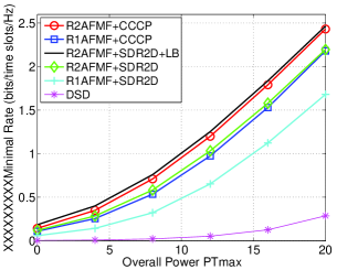
Figure 4: Minimum rate versus total power $P_{T,\max}$, first example.

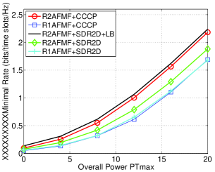
Figure 5: Minimum rate versus total power $P_{T,\max}$, first example.

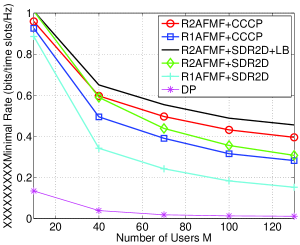
Figure 6: Minimum rate versus number of destinations $M$, first example.

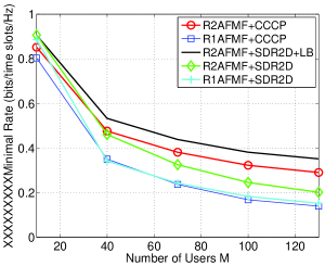
Figure 7: Minimum rate versus number of destinations $M$, first example.

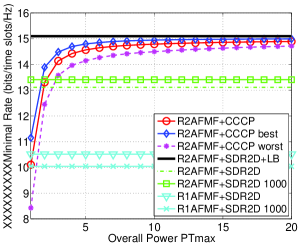
Figure 8: Minimum SNR versus number of iterations, second example.

V Conclusion

In this paper, a novel Rank-2-AFMS for single-group multicasting has been proposed. Our scheme generalizes the rank-one multicasting scheme of the literature to a rank-two multicasting scheme and allows to incorporate the direct channel from the source to the destinations in the detection. To select the proper source power and to adjust the relay weights we propose an iterative algorithm to maximize the lowest SNR at the destinations. The simulation results demonstrate that the proposed Rank-2-AFMS combined with the proposed iterative algorithm yields a performance close to the theoretical upper bound.

VI Acknowledgement

This work was supported by the Seventh Framework Programme for Research of the European Commission under grant number ADEL-619647.

References

- [1] A. B. Gershman, N. D. Sidiropoulos, S. Shahbazpanahi, M. Bengtsson, and B. Ottersten, “Convex optimization-based beamforming,” IEEE Signal Processing Magazine, vol. 27, no. 3, pp. 62–75, 2010.
- [2] Y. Jing and H. Jafarkhani, “Network beamforming using relays with perfect channel information,” IEEE Trans. Inform. Theory, vol. 55, pp. 2499–2517, June 2009.
- [3] Z. Ding, W. H. Chin, and K. K. Leung, “Distributed beamforming and power allocation for cooperative networks,” IEEE Trans. Wireless Commun., vol. 7, no. 5, pp.1817–1822, 2008.
- [4] P. Larsson, “Large-scale cooperative relaying network with optimal combining under aggregate relay power constraint,” Proc. of Future Telecom. Conf., Beijing, China, pp. 166-170, Dec. 2003.
- [5] V. Havary-Nassab, S. Shahbazpanahi, A. Grami, and Z.-Q. Luo, “Distributed beamforming for relay networks based on second-order statistics of the channel state information,” IEEE Trans. Signal Process., vol. 56, pp. 4306–4316, Sept. 2008.
- [6] H. Chen, A. B. Gershman, and S. Shahbazpanahi, “Filter-and-forward distributed beamforming in relay networks with frequency selective fading,” IEEE Trans. Signal Process., vol. 58, pp. 1251-1262, March 2010.
- [7] S. Fazeli-Dehkordy, S. Shahbazpanahi, and S. Gazor, “Multiple peer-to-peer communications using a network of relays,” IEEE Trans. Signal Process., vol. 57, pp. 3053–3062, Aug. 2009.
- [8] A. Schad and M. Pesavento, ”Multiuser bi-directional communications in cooperative relay networks,” Proc. IEEE CAMSAP’11, pp. 217–220, San Juan, Puerto Rico, Dec. 2011.
- [9] N. Bornhorst, M. Pesavento, and A. B. Gershman, “Distributed beamforming for multi-group multicasting relay networks,“ IEEE Trans. on Signal Process., vol. 60, no. 1, pp. 221–232, 2011.
- [10] A. Schad, K. L. Law, and M. Pesavento, ”A convex inner approximation technique for rank-two beamforming in multicasting relay networks,“ Proc. Eur. Signal Process. Conf., pp. 1369–1373, Aug. 2012.
- [11] A. Abdelkader, M. Pesavento, and A. B. Gershman, “Orthogonalization techniques for single group multicasting in cooperative amplify-and-forward networks,” Proceedings of the Fourth International Workshop on Computational Advances in Multi-Sensor Adaptive Processing (CAMSAP2011), San Juan, Puerto Rico, pp. 225–228, December 2011.
- [12] A. Schad, H. Chen, A. B. Gershman, and S. Shahbazpanahi, “Filter-and-forward peer-to-peer beamforming in relay networks with frequency selective channels,” Proceedings of the International Conference on Acoustics, Speech, and Signal Processing (ICASSP’10), Dallas, TX, USA, pp. 3246–3249 March 2010.
- [13] N. D. Sidiropoulos, T. N. Davidson, and Z.-Q. Luo, ”Transmit beamforming for physical-layer multicasting,“ IEEE Trans. on Signal Process., vol. 54, no. 6, pp. 2239–2251, Jun. 2006.
- [14] E. Karipidis, N. D. Sidiropoulos, and Z.-Q. Luo, ”Quality of service and max-min fair transmit beamforming to multiple co-channel multicast groups,“ IEEE Trans. Signal Process., vol. 56, pp. 1268–1279, Mar. 2008.
- [15] S. X. Wu, A. M. So, and W. K. Ma, “Rank-two transmit beamformed Alamouti space-time coding for physical-layer multicasting,” Proc. IEEE ICASSP’12, pp. 2793–2796, Kyoto, Japan, Mar. 2012.
- [16] X. Wen, K. L. Law, S. J. Alabed, and M. Pesavento, “Rank-two beamforming for single-group multicasting networks using OSTBC,” Proc. IEEE SAM’012, pp. 69–72, Hoboken, USA, June 2012.
- [17] S. Ji, S. X. Wu, A. M. So, and W. K. Ma, “Multi-group multicast beamforming in cognitive radio networks via rank-two transmit beamformed Alamouti space-time coding,” Proc. ICASSP’13, pp. 4409–4413, 2013.
- [18] X. Wu, W. K. Ma, and A. M. So, “Physical-layer multicasting by stochastic transmit beamforming and Alamouti space-time coding,” IEEE Trans. on Signal Process., vol. 61, no. 17, Sep. 2013.
- [19] K. L. Law, X. Wen, and M. Pesavento, “General-rank transmit beamforming for multi-group multicasting networks using OSTBC,” Proc. IEEE SPAWC’13, pp. 475–479, Jun. 2013.
- [20] Y. Silva and A. Klein, “Linear transmit beamforming techniques for the multigroup multicast scenario,” IEEE Trans. Vehicular Techn., vol. 58, pp. 4353–4367, 2009.
- [21] A. Abdelkader, A. B. Gershman, and N. D. Sidiropoulos, “Multiple-antenna multicasting using channel orthogonalization and local refinement,” IEEE Trans. Signal Process., vol. 58, pp. 3922–3927, 2010.
- [22] N. Bornhorst, P. Davarmanesh, and M. Pesavento, ”An extended interior-point method for transmit beamforming in multi-group multicasting,“ Proc. EUSIPCO’12, Bucharest, Romania, Aug. 2012.
- [23] K. Phan, T. Le-Ngoc, S. A. Vorobyov, and C. Tellambura, “Power allocation in wireless multi-user relay networks,” IEEE Trans. Wireless Commun., vol. 8, no. 5, pp. 2535-2545, 2009.
- [24] H. Al-Shatri and T. Weber, ”Optimizing power allocation in interference channels using D.C. programming,“ Proceedings of the Int. Symp. Modeling Optimization Mobile, Ad Hoc Wireless Netw., pp. 367–373, Jun. 2010.
- [25] K. Eriksson, S. Shi, N. Vucic, M. Schubert, and E. G. Larsson, ”Global optimal resource allocation for achieving maximum weighted sum rate,“ Proc. IEEE Global Telecommun. Conf., 2010.
- [26] H. H. Kha, H. D. Tuan, and H. H. Nguyen, “Fast global optimal power allocation in wireless networks by local d.c. programming,” IEEE Trans. Wireless Commun., vol. 11, pp. 510–515, Feb. 2012.
- [27] B. Song, Y.-H. Lin, and R. Cruz, ”Weighted max-min fair beamforming, power control, and scheduling for a MISO downlink,“ IEEE Trans. Wireless Commun., vol. 7, pp. 464–469, Feb. 2008.
- [28] Y. Cheng and M. Pesavento, ”Joint Optimization of Source Power Allocation and Distributed Relay Beamforming in Multiuser Peer-to-Peer Relay Networks,“ IEEE Trans. on Signal Process.,, vol. 60, no. 6, pp. 2962–2973, Jun. 2012.
- [29] A. Khabbazibasmenj, S. A. Vorobyov, F. Roemer, and M. Haardt, ”Polynomial-time DC (POTDC) for sum-rate maximization in two-way AF MIMO relaying,“ Proc. IEEE ICASSP’12, Kyoto, Japan, pp. 2889–2892, Mar. 2012.
- [30] A. Khabbazibasmenj, F. Roemer, S. A. Vorobyov, and M. Haardt, “Sum-rate maximization in two-way AF MIMO relaying: Polynomial time solutions to a class of DC programming problems,” IEEE Trans. Signal Process., vol. 60, no. 10, pp. 5478–5493, 2012.
- [31] H. H. Kha, H. D. Tuan, H. H. Nguyen, and T. T. Pham, “Optimization of cooperative beamforming for SC-FDMA multi-user multi-relay networks by tractable D.C. programming,” IEEE Trans. on Signal Process., vol. 61, pp. 467–479, Jan. 2013.
- [32] A. H. Phan, H. D. Tuan, and H. H. Kha, “D.C. Iterations for SINR Maximin Multicasting in Cognitive radio,” Proc. IEEE ICSPCS’12, pp. 1–5, Dec. 2012.
- [33] G. Dartmann, E. Zandi, and G. Ascheid, “A modified Levenberg-Marquardt method for the bidirectional relay channel,” available on http://arxiv.org/abs/1307.3121, Jul. 2013.
- [34] G. Dartmann and G. Ascheid, “Equivalent quasi-convex form of the multicast max-min beamforming problem,” IEEE Trans. on Vehicular Tech., vol. 62, no. 9, pp. 4643–4648, Nov. 2013.
- [35] Z.-Q. Luo and T.-H. Chang, ”SDP relaxation of homogeneous quadratic optimization: Approximation bounds and applications,“ Convex Opt. in Signal Process. and Comm., D. P. Palomar and Y. C. Eldar, Eds. Cambridge University Press, ch. 4, pp. 117–162, 2010.
- [36] S. M. Alamouti, ”A simple transmitter diversity scheme for wireless communications,“ IEEE J. Select. Areas Commun., vol. 16, pp.1451 – 1458, 1998.
- [37] V. Tarokh, H. Jafarkhani, and A. R. Calderbank, ”Space time block codes from orthogonal designs,“ IEEE Trans. Information Theory, vol. 45, no.5, pp. 1456–1467, Jul. 1999.
- [38] V. Tarokh, H. Jafarkhani, and A. R. Calderbank, ”Space–time block coding for wireless communications: Performance results,” IEEE J. Select. Areas Commun., vol. 17, pp. 451–460, Mar. 1999.
- [39] G. Ganesan and P. Stoica, ”Space-time block codes: A maximum SNR approach,” IEEE Trans. Inform. Theory, vol. 47, pp. 1650–1656, May 2001.
- [40] H. Jafarkhani, ”A quasi orthogonal space time block code,” IEEE Trans. Commun., vol. 49, pp. 1–4, Jan. 2001.
- [41] C. W. Tan and A. R. Calderbank, ”Multiuser detection of Alamouti signals,” IEEE Trans. Commun., vol. 57, no. 7, pp. 2080–2089, Jul. 2009.
- [42] D. Reynolds, X. Wang, and H. V. Poor, ”Blind adaptive space-time multiuser detection with multiple transmitter and receiver antennas,” IEEE Trans. Signal Process., vol. 50, no. 6, pp. 1261–1276, Jun. 2002.
- [43] S. Zhou and G. B. Giannakis, ”Optimal transmitter eigen-beamforming and space-time block coding based on channel mean feedback,” IEEE Trans. Signal Process., vol. 50, no. 10, pp. 2599–2613, Oct. 2002.
- [44] S. Zhou and G. B. Giannakis, ”Optimal transmitter eigen-beamforming and space-time block coding based on channel correlations,” IEEE Trans. Inform. Theory, vol. 49, no. 7, pp. 1673–1690, Jul. 2003.
- [45] C. Sun, N. C. Karmakar, K. S. Lim, and A. Feng, ”Combining beamforming with Alamouti scheme for multiuser MIMO communications,” Proc. of Veh. Technol. Conf., 2004.
- [46] L. Li, H. Jafarkhani, and S. A. Jafar, ”When Alamouti codes meet interference alignment: transmission schemes for two-user X channel,” in Proc. ISIT., Saint Pertersburg, Russia, 2011.
- [47] A. Zaki, C. Wang, and L. K. Rasmussen, ”Combining interference alignment and Alamouti codes for the 3-user MIMO interference channel,” IEEE WCNC’13, 2013.
- [48] D. Baum, J. Hansen, and J. Salo, “An interim channel model for beyond-3G systems: Extending the 3GPP spatial channel model,” Proceedings IEEE Veh. Technol. Conf., vol. 5, pp. 3132–3136, Jun. 2005.
- [49] Y. Jing and H. Jafarkhani, “Using orthogonal and quasi-orthogonal designs in wireless relay networks,” IEEE Trans. Inform. Theory, vol. 53, pp. 4106-4118, Nov. 2007.
- [50] B. Maham, A. Hjørungnes, and G. Abreu, “Distributed GABBA space-time codes in amplify-and-forward relay networks,“ IEEE Trans.Wireless Commun., vol. 8, no. 4, pp. 2036–2045, Apr. 2009.
- [51] E. Dahlman, S. Parkvall, and J. Sköld, ”LTE/LTE-Advanced for Mobile Broadband,“ Academic Press, 2011.
- [52] S. Boyd and L. Vandenberghe, Convex Optimization, Cambridge, U.K.: Cambridge Univ. Press, 2004.
- [53] R. Horst and N. V. Thoai, ”Dc programming: Overview,“ J. Optim. Theory Appl., vol. 103, no. 1, pp. 1–43, Oct. 1999.
- [54] B. K. Sriperumbudur and G. R. G. Lanckriet, ”On the convergence of the concave-convex procedure,“ Neural Inf. Process. Syst., pp. 1–9, 2009.
- [55] H. A. Le-Thi and T. Pham-Dinh, “Large scale molecular optimization from distance matrix by a d.c. optimization approach,” SIAM J. Optim., vol. 14, pp. 77–117, Jan. 2003.
- [56] L. T. H. An and P. D. Tao ”The DC (difference of convex functions) programming and DCA revisited with DC models of real world nonconvex optimization problems,“ 133. Annals of Operations Research, pp. 23–46, 2005.
- [57] H. Tuy, ”Convex analysis and global optimization,“ Boston: Kluwer Academic Publishers, 1998.
- [58] P. M. Pardalos and G. Schnitger, ”Checking local optimality in constrained quadratic programming is NP-hard,” Operations Research Letters, vol. 7, pp. 33—35, 1988.
- [59] C. W. Tan, M. Chiang, and R. Srikant, ”Maximizing sum rate and minimizing MSE on multiuser downlink: Optimality, fast algorithms and equivalence via max-min SINR,” IEEE Trans. on Signal Process., vol. 59, no. 12, pp. 6127–6143, 2011.
- [60] D. Cai, T. Q. Quek, and C. W. Tan, ”A unified analysis of max-min weighted SINR for MIMO downlink system,” IEEE Trans. on Signal Process., vol. 59, no. 8, pp. 3850–3862, 2011.
- [61] D. Cai, T. Q. Quek, C. W. Tan, and S. H. Low, ”Max-min SINR coordinated multipoint downlink transmission – duality and algorithms,” IEEE Trans. on Signal Process., vol. 60, no. 10, pp. 5384–5396, 2012.
- [62] M. Grant, S. Boyd, and Y. Ye, ”CVX: Matlab software for disciplined convex programming,“ available on http://www.stan- ford.edu/ boyd/cvx.
- [63] ”The MOSEK optimization toolbox for MATLAB manual. Version 7.0 (Revision 103),“ available on http://docs.mosek.com/7.0/toolbox/.
- [64] MATLAB optimization toolbox, U.K.: The Math Works Press, Aug. 2010, Release 2010 b.
- [65] R. J. Vanderbei and D. F. Shanno, ”An interior-point algorithm for nonconvex nonlinear programming,“ Comput. Optim. Appl., vol. 13, pp. 231–252, 1999.
- [66] P. E. Gill, W. Murray, and M. A. Saunders, ”SNOPT: An SQP algorithm for large-scale constrained optimization,“ SIAM Rev., vol. 47, no. 1, pp. 99–132, Mar. 2005.