Low-Complexity QL-QR Decomposition Based Beamforming Design for Two-Way MIMO Relay Networks

Abstract

In this paper, we investigate the optimization problem of joint source and relay beamforming matrices for a two-way amplify-and-forward (AF) multi-input multi-output (MIMO) relay system. The system consisting of two source nodes and two relay nodes is considered and the linear minimum mean-square-error (MMSE) is employed at both receivers. We assume individual relay power constraints and study an important design problem, a so-called determinant maximization (DM) problem. Since this DM problem is nonconvex, we consider an efficient iterative algorithm by using an MSE balancing result to obtain at least a locally optimal solution. The proposed algorithm is developed based on QL, QR and Choleskey decompositions which differ in the complexity and performance. Analytical and simulation results show that the proposed algorithm can significantly reduce computational complexity compared with their existing two-way relay systems and have equivalent bit-error-rate (BER) performance as the singular value decomposition (SVD) based on a regular block diagonal (RBD) scheme.

Index Terms: Two-way relay channel, MIMO, QL-QR decomposition, Choleskey decomposition, determinant maximization, amplify-and-forward.

I Introduction

Recently, wireless relay networks have been the focus of a lot of research because the relaying transmission is a promising technique which can be applied to extend the coverage or increase the system capacity. There are various cooperative relaying schemes have been proposed, such as amplify-and-forward (AF) [1] and [2], decode-and-forward (DF) [3], denoise-and-forward (DNF) [4], and compress-and-forward (CF) [5] cooperative relaying protocols. Among these approaches, AF is most widely used due to without detecting the transmitted signal. Therefore, an AF relay scheme requires a less processing power at the relays compared to other schemes.

In one-way relaying (OWR) approach, to completely exchange information between two base stations, four time slots are required in uplink (UL) and downlink (DL) communications, which leads to a loss of one-half spectral resources [6]. In order to solve this problem, a two-way relaying approach has been considered in [7], [8], and [9]. In a typical two-way relaying scheme, the communication is completed in two steps. First, the transmitters send their symbols to two relays, simultaneously. After receiving the signals, each relay processes them based on an efficient relaying scheme to produce new signals. Then the processed signals are broadcasted to both receiver nodes.

Multi-input multi-output (MIMO) relay systems have been investigated in [10]–[13]. It is shown that, by employing multiple antennas at the transmitter and/or the receiver, one can significantly improve the transmission reliability by leveraging spatial diversity. Relay precoder design methods have been investigated in [14], [15], [16]. A problem in designing optimal beamforming vectors for multicasting is challenging due to its nonconvex nature. In [14], the authors propose a transceiver precoding scheme at the relay node by using zero-forcing (ZF) and MMSE criteria with certain antenna configurations. The information theoretic capacity of the multi-antenna multicasting is studied in [15], along with the achievable rates using lower complexity transmission schemes, as the number of antennas or users goes to infinity. In [16], the authors propose an alternative method to characterize the capacity region of two-way relay channel (TWRC) by applying the idea of rate profile.

Joint optimization of the relay and source nodes for the MIMO TWRC have been studied in [9], [17]. In [9], the authors develop a unified framework for optimizing two-way linear non-regenerative MIMO relay systems and show that the optimal relay and source matrices have a general beamforming structure. The joint source node and relay precoding design for minimizing the mean squared error in a MIMO two-way relay (TWR) system is studied in [17].

Since singular value decomposition (SVD) and/or generalized SVD (GSVD) are widely used to find the orthogonal complement to solve an optimization problem [2], [9], [16], [29], but their computational complexities are extremely high. In order to reduce the complexity, the SVD can be replaced with a less complex QR decomposition [18] in this work. However, this approach leads to degrading the BER performance. In addition, it is difficult to realize in TWRC. In this paper, we investigate the joint source and relay precoding matrix optimization for a two way-relay amplify-and-forward relaying system where two source nodes and two relay nodes are equipped with multiple antennas. Also, in order to apply the QL/QR decomposition to the TWRC, we design a three part relay filter. Compared with existing works such as [9]–[14], the contributions of this paper can be summarized as follows. Firstly, we investigate a two-way MIMO relay system using the criteria which minimizes an MSE of the signal waveform estimation for both two source nodes. We prove an optimal sum-MSE solution can be obtained as the Winer filter while signal-to-noise-ratio (SNR) at both source nodes are equivalent [20] which leading to an MSE balancing result. Secondly, we propose a new cooperative scenario, i.e., the QL-QR compare with the Choleskey decomposition which significantly reduces the computational complexity of the optimal design. In this proposed design, the channels of its left side are decomposed by the QL decomposition while those of its right side factorized by the QR decomposition. And the equivalent noise covariance is decomposed by the Choleskey decomposition. We also design the three part relay filter, which is comprised by a left filer, a middle filter, and a right filter, to efficiently combine two source nodes and the relay nodes. By these approaches, the received signals at both two source nodes are able to be redeemed as either lower or upper triangular matrices. Stemming from one of the properties of triangular matrices such that their determinant is identical to the multiplication of their eigenvalues, we are able to straightforwardly solve the optimization problem as a determinant maximization problem. Also, we can obtain the BER performance equivalent to that of SVD-RBD scheme.

The rest of this paper is organized as follows. Section II describes a system model of the TWRC and raises a sum-MSE problem. In Section III, we propose an iterative QL-QR algorithm and a joint optimal beamforming design. In Sections IV, we discuss the computational complexity of an efficient channel model. The simulation results are presented to show the excellent performance of our proposed algorithm for the TWRC in Section V. Section VI concludes this paper.

Notations: $\mathbf{A}^{*}$ and $\mathbf{A}^{T}$ denote the conjugate and the transpose of a matrix $\mathbf{A}$, respectively. $\mathbf{d}(.)$ denotes a diagonal matrix and an $N\times N$ identity matrix is denoted by $\mathbf{I}_{N}$. $\mathrm{E}(.)$ stands for the statistical expectation and $(.)^{H}$ denotes a Hermitian transpose of a given matrix. $tr(.)$ and $R(.)$ denotes matrix trace and the range of a matrix.

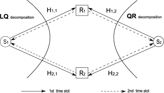
Figure 1: Proposed LQ-QR Amplify-and-Forward MIMO TWR system.

II System Model and Sum-MSE

We consider a TWRC consisting of two source nodes $\mathbf{S}_{1}$ and $\mathbf{S}_{2}$, and two relay nodes $\mathbf{R}_{1}$ and $\mathbf{R}_{2}$ as shown in Fig. 1. The source and relay nodes are equipped with M and N antennas, respectively. We adopt the relay protocol with two time slots introduced in [14]. In the first time slot, the information vector $x_{i}\in{\mathbb{C}^{M\times{1}}}$ is linearly processed by a precoding matrix $\mathbf{V}_{i}\in{\mathbb{C}^{M\times{M}}}$ and then be transmitted to the relay nodes. The received signals at $\mathbf{R}_{i}$, $i\in{\{1,2\}}$, can be expressed as

$$y_{R_{1}}=\textbf{H}_{1,1}s_{1}+\textbf{H}_{1,2}s_{2}+n_{R_{1}}$$

$$y_{R_{2}}=\textbf{H}_{2,1}s_{1}+\textbf{H}_{2,2}s_{2}+n_{R_{2}},$$ (1)

where $y_{R_{i}}\in{\mathbb{C}^{N\times 1}},i\in\{1,2\}$, indicates the received signal vector, $\textbf{H}_{i,j}\in{\mathbb{C}^{N\times{M}}},i,j\in\{1,2\}$, represents the channel matrix from source $j$ to relay $i$, as shown in Fig.1, $s_{i}\in{\mathbb{C}^{M\times 1}}$ is the transmitted symbol vector from $\mathbf{S}_{i}$, and $n_{R_{i}}\sim{CN(0,\sigma^{2}_{R_{i}}\mathbf{I}_{N})}$ represents the additive white Gaussian noise (AWGN) vector with zero mean and variance $\sigma^{2}_{R_{i}}$ at relay node $i$. The term $s_{i}$ is subject to a power constraint, $tr\{E(s_{i}s^{H}_{i})\}\leq{P_{i}}$ with $tr\{E(x_{i}x^{H}_{i})\}\leq{\frac{P_{i}}{M}\mathbf{I}_{M}}$, where $P_{i}$ is the transmit power at $\mathbf{S}_{i}$.

To find an appropriate power normalization vector $\rho_{R}$, we express the total transmission power at the source node with $\mathbf{V}_{i}$ as

$$tr\{\mathbf{V}_{1}\mathbf{V}^{H}_{1}\!+\!\mathbf{V}_{2}\mathbf{V}^{H}_{2}\}\!\!\!\! = \!\!\!\!tr\left\{\rho^{2}_{R}\left(\textbf{V}^{b}_{1}\left(\textbf{V}^{b}_{1}\right)^{H}+\textbf{V}^{b}_{2}\left(\textbf{V}^{b}_{2}\right)^{H}\right)\right\}$$ (2)

$$= \!\!\!\!tr\left\{\rho^{2}_{R}\left(P_{1}+P_{2}\right)\right\}.$$

In this paper, we assume that each transmit antenna satisfies the unity transmission power constraint. To satisfy the power constraint, we propose the following power normalization vector

$$\rho_{R}=1/\sqrt{P_{1}+P_{2}}.$$ (3)

In the second time slot, after power normalization, the relay node $\mathbf{R}_{i}$ linearly amplifies $y_{R_{i}}$ with an $N\times{N}$ matrix $\mathbf{F}_{i}$ and then broadcasts the amplified signal vector $x_{R_{i}}$ to source nodes 1 and 2. The signals transmitted from relay node $i$ can be expressed as

$$x_{R_{i}}=\rho_{R}\textbf{F}_{i}y_{R_{i}}.$$ (4)

Using (II) and (4), the received signal vectors at $\mathbf{S}_{1}$ and $\mathbf{S}_{2}$ can be, respectively, written as

$$y_{1} = \textbf{H}^{T}_{1,1}\textbf{F}_{1}\textbf{H}_{1,2}s_{1}+\textbf{H}^{T}_{1,1}\textbf{F}_{1}\textbf{H}_{1,2}s_{2}+\textbf{H}^{T}_{2,1}\textbf{F}_{2}\textbf{H}_{2,2}s_{1}$$

$$+\textbf{H}^{T}_{2,1}\textbf{F}_{2}\textbf{H}_{2,2}s_{2}+\textbf{H}^{T}_{1,1}\textbf{F}_{1}n_{R_{1}}+\textbf{H}^{T}_{2,1}\textbf{F}_{2}n_{R_{2}}+n_{1}$$

$$y_{2} = \textbf{H}^{T}_{1,2}\textbf{F}_{1}\textbf{H}_{1,1}s_{1}+\textbf{H}^{T}_{1,2}\textbf{F}_{1}\textbf{H}_{1,1}s_{2}+\textbf{H}^{T}_{2,2}\textbf{F}_{2}\textbf{H}_{2,1}s_{1}$$

$$+\textbf{H}^{T}_{2,2}\textbf{F}_{2}\textbf{H}_{2,1}s_{2}+\textbf{H}^{T}_{1,2}\textbf{F}_{1}n_{R_{1}}+\textbf{H}^{T}_{2,2}\textbf{F}_{2}n_{R_{2}}+n_{2},$$

where ${\textbf{H}}^{T}_{i,j}$, $i,j\in\{1,2\}$, indicates the $M\times{N}$ channel matrix from the relay node $i$ to the source node $j$, and $n_{i}$, $i\in\{1,2\},$ is an $M\times 1$ noise vector at $\mathbf{S}_{i}$. We assume that the relay nodes perfectly know the channel state information (CSI) of $\textbf{H}_{i,j}$. The relay node $\mathbf{R}_{i}$ performs the optimizations of $\textbf{F}_{i}$ and $\mathbf{V}_{i}$, and then transmits the information to the source nodes 1 and 2. Since source node $i$ knows its own transmitted signal vector $s_{i}$ and full CSI, the self-interference components in (II) can be efficiently cancelled. The effective received signal vectors are given by

$$\widetilde{y}_{1} = \textbf{H}^{T}_{1,1}\textbf{F}_{1}\textbf{H}_{1,2}s_{2}+\textbf{H}^{T}_{2,1}\textbf{F}_{2}\textbf{H}_{2,2}s_{2}+\textbf{H}^{T}_{1,1}\textbf{F}_{1}n_{R_{1}}$$ (6)

$$+\textbf{H}^{T}_{2,1}\textbf{F}_{2}n_{R_{2}}+n_{1}$$

$$= \mathbf{\widetilde{H}}_{1}s_{2}+\widetilde{n}_{1},$$

$$\widetilde{y}_{2} = \textbf{H}^{T}_{1,2}\textbf{F}_{1}\textbf{H}_{1,1}s_{1}+\textbf{H}^{T}_{2,2}\textbf{F}_{2}\textbf{H}_{2,1}s_{1}+\textbf{H}^{T}_{1,2}\textbf{F}_{1}n_{R_{1}}$$ (7)

$$+\textbf{H}^{T}_{2,2}\textbf{F}_{2}n_{R_{2}}+n_{2}$$

$$= \mathbf{\widetilde{H}}_{2}s_{1}+\widetilde{n}_{2},$$

where $\widetilde{\textbf{H}}_{1}=\textbf{H}^{T}_{1,1}\textbf{F}_{1}\textbf{H}_{1,2}+\textbf{H}^{T}_{2,1}\textbf{F}_{2}\textbf{H}_{2,2}$ and $\widetilde{\textbf{H}}_{2}=\textbf{H}^{T}_{1,2}\textbf{F}_{1}\textbf{H}_{1,1}+\textbf{H}^{T}_{2,2}\textbf{F}_{2}\textbf{H}_{2,1}$ are the equivalent MIMO channels seen at source nodes $\mathbf{S}_{1}$ and $\mathbf{S}_{2}$, respectively. The vectors $\widetilde{n}_{1}=\textbf{H}^{T}_{1,1}\textbf{F}_{1}n_{R_{1}}+\textbf{H}^{T}_{2,1}\textbf{F}_{2}n_{R_{2}}+n_{1}$ and $\widetilde{n}_{2}=\textbf{H}^{T}_{1,2}\textbf{F}_{1}n_{R_{1}}+\textbf{H}^{T}_{2,2}\textbf{F}_{2}n_{R_{2}}+n_{2}$ are the equivalent noises at source node $\mathbf{S}_{1}$ and $\mathbf{S}_{2}$, respectively.

Due to the lower computational complexity, linear receivers are applied at source node $i$ to retrieve the transmitted signals sent from the other nodes. The estimated signal waveform vector is given as $\widehat{s}_{\overline{i}}=\mathbf{W}^{H}_{i}\widetilde{y}_{i}$, where $\mathbf{W}_{i}$ is an $M\times{M}$ weight matrix, with $\overline{i}=2$ for $i=1$ and $\overline{i}=1$ for $i=2$. From (6), the MSE matrix of the signal waveform estimation denoted by $\mathbf{MSE}_{\overline{i}}=\mathrm{E}[(\widehat{s}_{i}-{s}_{i})(\widehat{s}_{i}-{s}_{i})^{H}]$, which can be further written as

$$\mathbf{MSE}_{i} = (\mathbf{W}^{H}_{i}\widetilde{\mathbf{H}}_{i}-\mathrm{I}_{M})(\mathbf{W}^{H}_{i}\widetilde{\mathbf{H}}_{i}-\mathrm{I}_{M})^{H}$$ (8)

$$+\mathbf{W}^{H}_{i}\mathbf{C}_{n_{i}}\mathbf{W}_{i}$$

where $\mathbf{C}_{n_{i}}=\textbf{H}^{T}_{i,i}\textbf{F}_{i}\textbf{F}^{H}_{i}\textbf{H}^{*}_{i,i}+\textbf{H}^{T}_{\overline{i},i}\textbf{F}_{\overline{i}}\textbf{F}^{H}_{\overline{i}}\textbf{H}^{*}_{\overline{i},i}+\mathbf{I}_{M}$ is the equivalent noise covariance. The sum-MSE of the two source nodes in the proposed system model can be written as:

$$\mathbf{MSE}_{sum}=\mathbf{MSE}_{1}+\mathbf{MSE}_{2}.$$ (9)

Note that the sum-MSE minimization criterion measures the overall transmission performance of both the DL and the UL. Since the two data streams are transmitted at different directions during the two time slots are considered in the TWR network.

III Joint Source and relay Beamforming Design

In this section, we develop an iterative QL-QR algorithm by using the MSE balancing result. The QL-QR algorithm involves two steps, i.e., the linear receiver matrix optimization and the joint source and relay beamformer design.

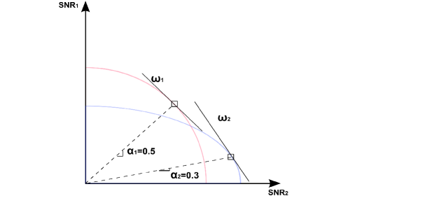
Figure 2: Examples of the SNR regions achieved in a TWRC with two relays.

III-A Proposed Optimal Detector and Optimization Problem

We would like to find the jointly optimal beamforming vectors $\mathbf{W}_{i}$, $\mathbf{V}_{i}$ and $\mathbf{F}_{i}$ such as the following sum-MSE is minimized

$$\min\limits_{\mathbf{W}_{1},\mathbf{W}_{2},\mathbf{F}_{1},\mathbf{F}_{2},\mathbf{V}_{1},\mathbf{V}_{2}}~{}~{}\mathbf{MSE}_{sum}.$$ (10)

According to (4), we consider the following transmission power constraint at relay node

$$tr{\left(\textbf{F}_{1}\textbf{D}_{1}\textbf{F}^{H}_{1}+\textbf{F}_{2}\textbf{D}_{2}\textbf{F}^{H}_{2}\right)}\leq{P_{R_{1}}+P_{R_{2}}=P_{R}},$$ (11)

where $\textbf{D}_{1}=\rho^{2}_{R}(\textbf{H}_{1,1}\mathbf{V}_{1}\mathbf{V}^{H}_{1}\textbf{H}^{H}_{1,1}+\textbf{H}_{1,2}\mathbf{V}_{2}\mathbf{V}^{H}_{2}\textbf{H}^{H}_{1,2}+\mathbf{I}_{N})$ and $\textbf{D}_{2}=\rho^{2}_{R}(\textbf{H}_{2,1}\mathbf{V}_{1}\mathbf{V}^{H}_{1}\textbf{H}^{H}_{2,1}+\textbf{H}_{2,2}\mathbf{V}_{2}\mathbf{V}^{H}_{2}\textbf{H}^{H}_{2,2}+\mathbf{I}_{N})$. The $P_{R_{i}}$ denotes the power constraint at the relay node $\mathbf{R}_{i}$, and $P_{R}$ is the total relay power. The transmission power constraint at two source nodes can be written as

$$tr{(\mathbf{V}_{i}\mathbf{V}^{H}_{i})}\leq{P_{i}},~{}~{}~{}~{}~{}i=1,2$$ (12)

where $P_{i}$ is the available power at the $i$th source node. According to (10), (11) and (12), the joint optimization problem of the sum-MSE can be formulated as follows:

$$\min\limits_{\mathbf{W}_{1},\mathbf{W}_{2},\mathbf{F}_{1},\mathbf{F}_{2},\mathbf{V}_{1},\mathbf{V}_{2}} ~{}~{}~{}~{}~{}~{}~{}~{}~{}~{}~{}~{}\mathbf{MSE}_{sum}$$ (13)

$$s.t. ~{}tr{\left(\textbf{F}_{1}\textbf{D}_{1}\textbf{F}^{H}_{1}+\textbf{F}_{2}\textbf{D}_{2}\textbf{F}^{H}_{2}\right)}\leq{P_{R}}$$

$$s.t. ~{}~{}~{}~{}~{}~{}~{}~{}tr{(\mathbf{V}_{i}\mathbf{V}^{H}_{i})}\leq{P_{i}}.$$

It is shown in [20] that at the optimum, $SNR_{1}=SNR_{2}$ holds true, thus leading to an SNR balancing result. Otherwise, if $SNR_{1}>SNR_{2}$, then $P_{2}$ can be reduced to retain $SNR_{1}=SNR_{2}$, and this reduction of $P_{2}$ will not violate the power constraint, i.e.,

$$P_{1}\cdot SNR_{1}=P_{2}\cdot SNR_{2}.$$ (14)

In Fig. 2, we show two examples of the SNR regions with $\alpha_{1}=0.5$ and $\alpha_{2}=0.3$, where $\omega_{i}\in[0,1]$ is a Lagrange multiplier weight value and $\alpha_{i}\in[0,1]$ is an SNR weight value. We have assumed the sum of SNR is a constant value. It is clear that the SNR region of $\alpha_{1}$ is larger than that of $\alpha_{2}$. For further details, see [20]. As discussed in [21], the optimization problems have the performance matrix that are functions of SNR , namely the MSE at the output of a linear-MMSE (LMMSE) filter of each user

$$\mathbf{MSE}=\frac{1}{1+SNR}.$$ (15)

By these two approaches, the max-min optimization problem in (13) can be efficiently written as

$$\min\limits_{\mathbf{W}_{1},\mathbf{F}_{i},\mathbf{V}_{2}} ~{}~{}~{}~{}~{}~{}~{}~{}~{}~{}~{}~{}\mathbf{MSE}_{1}$$ (16)

$$s.t. ~{}tr{(\textbf{F}_{1}\textbf{D}_{1}\textbf{F}^{H}_{1}+\textbf{F}_{2}\textbf{D}_{2}\textbf{F}^{H}_{2}})\leq{P_{R}}$$ (17)

$$s.t. ~{}~{}~{}~{}~{}~{}\mathbf{MSE}_{1}=\mathbf{MSE}_{2},$$ (18)

where $i\in{1,2}$. Since the optimization problem (16) is nonconvex, it is difficult to obtain the globally optimal solution. In this paper, we present a locally optimal solution of the joint optimization problem over $\mathbf{W}_{i}$, $\mathbf{V}_{i}$ and $\mathbf{F}_{i}$ where $i=1,2$, which can be solved by three stages, i.e., $1:$ The linear receiver weighted matrices are optimized with the fixed source precoding matrix $\mathbf{V}_{i}$ and relay amplifying matrices $\mathbf{F}_{i}$ ($\mathbf{W}_{i}$ is not in constraints (17) and (18)). $2:$ With given $\mathbf{W}_{i}$ and fixed $\mathbf{F}_{i}$, update $\mathbf{V}_{i}$. $3:$ With given $\mathbf{W}_{i}$ and $\mathbf{V}_{i}$, obtain suboptimal $\mathbf{F}_{i}$ to solve (16).

Lemma 1 : For any fixed $\mathbf{V}_{i}$ and $\mathbf{F}_{i}$, the minimization problems in (16) are convex quadratic problems and the optimal $\mathbf{W}_{i}$ can be obtained as the Wiener filter which is used to decode $s_{i}$ shown as follows

$$\mathbf{W}^{o}_{i}=(\mathbf{\widetilde{H}}_{i}\mathbf{\widetilde{H}}^{H}_{i}+\mathbf{C}_{n_{i}})^{-1}\mathbf{\widetilde{H}}_{i},$$ (19)

Proof: For source node $i$, the MSE can be further expressed as:

$$\mathbf{MSE}_{i} = \mathbf{W}^{H}_{i}\widetilde{\mathbf{H}}_{i}\widetilde{\mathbf{H}}^{H}_{i}\mathbf{W}_{i}-\mathbf{W}^{H}_{i}\widetilde{\mathbf{H}}_{i}-\widetilde{\mathbf{H}}^{H}_{i}\mathbf{W}_{i}$$ (20)

$$+\mathbf{I}_{M}+\mathbf{W}^{H}_{i}\mathbf{C}_{n_{i}}\mathbf{W}_{i}$$

Based on (20), the derivation of an optimal MSE detection matrix $\mathbf{W}^{opt}_{i}$ is equivalent to solving the following equation:

$$\frac{\partial\mathbf{MSE}_{i}}{\partial\mathbf{W}^{H}_{i}}=2\widetilde{\mathbf{H}}_{i}\widetilde{\mathbf{H}}^{H}_{i}\mathbf{W}_{i}-2\widetilde{\mathbf{H}}_{i}+2\mathbf{C}_{n_{i}}\mathbf{W}_{i}=0.$$ (21)

Then, we may obtain closed-form solution of $\mathbf{W}_{i}$, which is

$$\mathbf{W}^{o}_{i}=(\mathbf{\widetilde{H}}_{i}\mathbf{\widetilde{H}}^{H}_{i}+\mathbf{C}_{n_{i}})^{-1}\mathbf{\widetilde{H}}_{i}.$$ (22)

This completes the proof.

With the optimal $\mathbf{W}^{o}_{1}$ fixed, the outer minimization problem in (16) can be rewritten as

$$\min\limits_{\mathbf{F}_{1},\mathbf{F}_{2},\mathbf{V}_{1},\mathbf{V}_{2}} ~{}~{}~{}~{}~{}~{}~{}~{}~{}~{}~{}~{}\mathbf{MSE}^{o}_{1}$$ (23)

$$s.t. ~{}tr{(\textbf{F}_{1}\textbf{D}_{1}\textbf{F}^{H}_{1}+\textbf{F}_{2}\textbf{D}_{2}\textbf{F}^{H}_{2})}\leq{P_{R}}$$

$$s.t. ~{}~{}~{}~{}~{}~{}~{}\mathbf{MSE}_{1}=\mathbf{MSE}_{2},$$

where $\mathbf{MSE}^{o}_{1}$ is the MSE matrix using $\mathbf{W}^{o}_{1}$. By substituting (19) into (8), we have

$$\mathbf{MSE}^{o}_{1}=[\mathbf{I}_{M}+\mathbf{\widetilde{H}}^{H}_{1}\mathbf{C}^{-1}_{n_{1}}\mathbf{\widetilde{H}}_{1}]^{-1}.~{}~{}~{}i=1,2.$$ (24)

Note that the matrix inversion lemma is used to obtain (24).

III-B Joint Optimal Source and Relay Beamforming Matrices Design and Iterative Algorithm

In this section, we focus on the source and relay beamforming matrices design and develop an iterative algorithm which is suboptimal for the general case, but has a much lower computational complexity. For the fixed $\mathbf{F}_{i}$, the source precoding matrix $\mathbf{V}_{i}$ is optimized by solving the following problem

$$\min\limits_{\mathbf{V}_{1},\mathbf{V}_{2}} ~{}~{}~{}~{}~{}~{}~{}~{}~{}~{}~{}~{}tr\left[\mathbf{I}_{M}+\mathbf{V}^{H}_{2}\mathbf{\Phi}\mathbf{V}_{2}\right]^{-1}$$ (25)

$$s.t. ~{}~{}~{}tr\{\rho^{2}_{R}(\textbf{V}^{H}_{1}\mathbf{\Psi}_{1}\textbf{V}_{1}+\textbf{V}^{H}_{2}\mathbf{\Psi}_{2}\textbf{V}_{2})\}\leq{P_{R}}$$

$$s.t. ~{}~{}~{}~{}~{}~{}~{}~{}~{}~{}~{}~{}~{}~{}~{}~{}tr\{\mathbf{V}^{H}_{i}\mathbf{V}_{i}\}\leq P_{i},$$

where $\mathbf{\Phi}=\mathbf{\widehat{H}}^{H}_{1}\mathbf{\widehat{C}}^{-1}_{1}\mathbf{\widehat{H}}_{1}$ , $\mathbf{\Psi}_{1}=\mathbf{H}^{H}_{1,1}\mathbf{F}^{H}_{1}\mathbf{F}_{1}\mathbf{H}_{1,1}+\mathbf{H}^{H}_{2,1}\mathbf{F}^{H}_{2}\mathbf{F}_{2}\mathbf{H}_{2,1}$, and $\mathbf{\Psi}_{2}=\mathbf{H}^{H}_{1,2}\mathbf{F}^{H}_{1}\mathbf{F}_{1}\mathbf{H}_{1,2}+\mathbf{H}^{H}_{2,2}\mathbf{F}^{H}_{2}\mathbf{F}_{2}\mathbf{H}_{2,2}$. The Lagrangian function associated with the problem (25) is given by

$$L_{\mathbf{V}} = tr\left[\mathbf{I}_{M}+\mathbf{V}^{H}_{2}\mathbf{\Phi}\mathbf{V}_{2}\right]^{-1}+\sum^{2}_{i=1}\mu_{i}\left(tr\{\mathbf{V}^{H}_{i}\mathbf{V}_{i}\}-P_{i}\right)$$ (26)

$$+\mu_{3}\left\{tr\{\rho^{2}_{R}(\textbf{V}^{H}_{1}\mathbf{\Psi}_{1}\textbf{V}_{1}+\textbf{V}^{H}_{2}\mathbf{\Psi}_{2}\textbf{V}_{2})\}-P_{R}\right\},$$

where $\mu_{i}\geq 0$ is the Lagrange multiplier.

Case 1: When $\mu_{i}=0$, making the derivative of $L_{\mathbf{V}}$ with respect to $\mathbf{V}_{2}$ be zero, we obtain

$$\frac{\partial L_{\mathbf{V}}}{\partial\mathbf{V}_{2}}=-\left[\mathbf{I}_{M}+\mathbf{V}^{H}_{2}\mathbf{\Phi}\mathbf{V}_{2}\right]^{-2}\mathbf{V}^{H}_{2}\mathbf{\Phi}=0.$$ (27)

Since $\mathbf{V}_{2}$ and $\mathbf{\Phi}$ are nonsingular matrices, (27) can be represented as

$$\mathbf{I}_{M}+\mathbf{V}^{H}_{2}\mathbf{\Phi}\mathbf{V}_{2}=0.$$ (28)

Simplifying (28), $\mathbf{I}_{M}>0$ and $\mathbf{V}^{H}_{2}\mathbf{\Phi}\mathbf{V}_{2}\geq 0$. Consequently, in Case 1, the optimal solution is not existent.

Case 2: When $\mu_{i}>0$, we rewrite the Lagrangian function as

$$L_{\mathbf{V}} = \!\!\!\!\left[\mathbf{I}_{M}+\mathbf{V}^{H}_{2}\mathbf{\Phi}\mathbf{V}_{2}\right]^{-1}-\mu_{1}P_{1}-\mu_{2}P_{2}-\mu_{3}P_{R}$$ (29)

$$\!\!\!\!+\mathbf{V}^{H}_{2}\Upsilon\Upsilon^{H}\mathbf{V}_{2}\!+\!\mu_{3}\rho^{2}_{R}\mathbf{V}_{1}^{H}\mathbf{\Psi}_{1}\mathbf{V}_{1}\!+\!\mu_{1}\mathbf{V}_{1}^{H}\mathbf{V}_{1}\!,$$

where $\Upsilon\Upsilon^{H}=\mu_{2}\mathbf{I}_{M}+\mu_{3}\rho^{2}_{R}\mathbf{\Psi}_{2}$. We obtain the derivative of $L_{\mathbf{V}}$ as

$$\frac{\partial L_{\mathbf{V}}}{\partial\mathbf{V}_{2}}=-\left[\mathbf{I}_{M}+\mathbf{V}^{H}_{2}\mathbf{\Phi}\mathbf{V}_{2}\right]^{-2}\mathbf{V}^{H}_{2}\mathbf{\Phi}+\mathbf{V}^{H}_{2}\Upsilon\Upsilon^{H}=0.$$ (30)

Since $\mathbf{V}^{H}_{2}$ and $\mathbf{\Phi}$ are nonsingular matrices, multiply both sides by $\left(\mathbf{V}^{H}_{2}\right)^{-1}$ and $\mathbf{\Phi}^{-1}$, we have

$$\left(\mathbf{V}^{H}_{2}\right)^{-1}\left[\mathbf{I}_{M}+\mathbf{V}^{H}_{2}\mathbf{\Phi}\mathbf{V}_{2}\right]^{-2}\mathbf{V}^{H}_{2}=\Upsilon\Upsilon^{H}\mathbf{\Phi}^{-1}.$$ (31)

Due to $\mathbf{\Phi}$ is Hermitian and positive definite, we apply the Choleskey decomposition of $\mathbf{\Phi}=\Omega^{H}\Omega$, where $\Omega$ is a lower triangular matrix. Consequently, we represent (31) as

$$\left(\Omega^{H}\right)^{-1}\left(\mathbf{V}^{H}_{2}\right)^{-1}\left[\mathbf{I}_{M}+\mathbf{V}^{H}_{2}\Omega^{H}\Omega\mathbf{V}_{2}\right]^{-2}\mathbf{V}^{H}_{2}\Omega^{H}$$ (32)

$$= \left(\Omega^{H}\right)^{-1}\Upsilon\Upsilon^{H}\left(\Omega^{H}\Omega\right)^{-1}\Omega^{H}.$$

By the definition of the matrix identity as

$$\left[\mathbf{I}_{M}+\mathbf{X}\mathbf{X}^{H}\right]^{-1}\mathbf{X}=\mathbf{X}\left[\mathbf{I}_{N}+\mathbf{X}^{H}\mathbf{X}\right]^{-1},$$ (33)

for any $M\times N$ matrix $\mathbf{X}$, we can rewrite (32) as

$$\left[\mathbf{I}_{M}+\Omega\mathbf{V}_{2}\mathbf{V}^{H}_{2}\Omega^{H}\right]^{-2}=\left(\Omega^{H}\right)^{-1}\Upsilon\Upsilon^{H}\Omega^{-1}.$$ (34)

Solving (35) for $\mathbf{V}_{2}$, we obtain (32) as

$$\mathbf{V}_{2}=\left(\nabla\nabla^{H}-\mathbf{\Phi}^{-1}\right)^{\frac{1}{2}},$$ (35)

where $\nabla=\left(\Upsilon^{H}\Omega\right)^{-\frac{1}{2}}$. Obviously, the precoding matrix ${\textbf{V}}_{1}$ can be obtained in the same way.

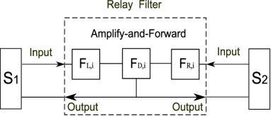
Figure 3: The relay filter design of the proposed QL-QR technique.

Figure 3 shows our proposed relay filter design, which forwards the received signal (input) from $\mathbf{S}_{1}$ amplified by a Left Filter (LF) matrix $\mathbf{F}_{L,i}$ and the signal from $\mathbf{S}_{2}$ amplified by a Right Filter (RF) matrix $\mathbf{F}_{R,i}$ to the Center Filter (CF) $\mathbf{F}_{D,i}$ that amplifies the outputs from the Left Filter (LF) matrix $\mathbf{F}_{L,i}$ and the Right Filter (RF) matrix $\mathbf{F}_{R,i}$, and forward them to $\mathbf{S}_{1}$ and $\mathbf{S}_{2}$ (output).

Lemma 2: The optimal relay filter constructive of $\mathbf{F}_{L}$, $\mathbf{F}_{R}$ and $\mathbf{F}_{D}$ matrices i.e., for $\mathbf{R}_{1}$ and $\mathbf{R}_{2}$ can be designed as

$$\mathbf{F}_{L,1}=\mathbf{Q}^{*}_{L,1},~{}\mathbf{F}_{L,2}=\mathbf{Q}^{*}_{L,2},$$

$$\mathbf{F}_{R,1}=\mathbf{Q}^{H}_{R,1},~{}\mathbf{F}_{R,2}=\mathbf{Q}^{H}_{R,2},$$

$$\mathbf{F}_{D,1}~{}\mathrm{and}~{}\mathbf{F}_{D,2}~{}\mathrm{are~{}diagonal~{}matrix}.$$ (36)

Proof: For $\mathbf{F}_{L,i}$ and $\mathbf{F}_{R,i}$, the proof is similar as Theorem 3.1 in [22]. For $\mathbf{F}_{D,i}$, using Theorem 2 in [9], the structure of $\mathbf{F}_{D,i}$ is optimal for the two cases of

$$(a):~{}~{}~{}~{}~{}R(\mathbf{H}_{1}\mathbf{V}_{1})\bot R(\mathbf{H}_{2}\mathbf{V}_{2});(\mathbf{H}^{*}_{1})\bot R(\mathbf{H}^{*}_{2})$$

$$~{}~{}\mathrm{and}~{}\,~{}~{}~{}R(\mathbf{H}_{3}\mathbf{V}_{1})\bot R(\mathbf{H}_{4}\mathbf{V}_{2});(\mathbf{H}^{*}_{3})\bot R(\mathbf{H}^{*}_{4})$$

$$(b):~{}~{}~{}~{}~{}R(\mathbf{H}_{1}\mathbf{V}_{1})\|R(\mathbf{H}_{2}\mathbf{V}_{2});(\mathbf{H}^{*}_{1})\bot R(\mathbf{H}^{*}_{2})$$

$$~{}~{}\mathrm{and}~{}\,~{}~{}~{}R(\mathbf{H}_{1}\mathbf{V}_{1})\|R(\mathbf{H}_{2}\mathbf{V}_{2});(\mathbf{H}^{*}_{1})\bot R(\mathbf{H}^{*}_{2}).$$ (37)

Case a: If $N=2$, the optimal $\mathbf{F}_{D,i}$ is a diagonal matrix given as

$$\mathbf{F}_{D,i} \triangleq {\left[\begin{array}[]{cc}\mathbf{f}_{d,i,1}&\mathbf{0}\\ \mathbf{0}&\mathbf{f}_{d,i,2}\\ \end{array}\right]}.$$ (40)

If $N=2a$, $a={2,3,...}$, the optimal $\mathbf{F}_{D,i}$ is a $2\times 2$ block diagonal matrix given as

$$\mathbf{F}_{D,i} \triangleq {\left[\begin{array}[]{cc}\mathbf{F}_{D,i,1}&\mathbf{0}\\ \mathbf{0}&\mathbf{F}_{D,i,2}\\ \end{array}\right]},$$ (43)

where $\mathbf{F}_{D,i,1}$ and $\mathbf{F}_{D,i,2}$ are $\frac{N}{2}\times\frac{N}{2}$ matrices.
Case b: The optimal $\mathbf{F}_{D,i}$ is defined as

$$\mathbf{F}^{\star}_{D,i} \triangleq {\left[\begin{array}[]{cc}\mathbf{f}_{d,i,1}\\ \mathbf{f}_{d,i,2}\\ \end{array}\right]}.$$ (46)

Discussion: In Case b, since $\mathbf{F}^{\star}_{D,i}$ is optimal, but the computational complexity will be considerably increased compared with Case a, so we exclude it.

For Case a, Before we develop a numerical method to solve vector $\mathbf{F}_{D,i}$, let us have some insights into the structure of this suboptimal relay beamforming matrix. To simplify relay beamforming matrix $\mathbf{F}_{D,i}$, we introduce a following property:

Property 1: The statistical behavior of a unitary matrix $\mathbf{U}$ remains unchanged when multiplied by any unitary matrix $\mathbf{T}$ independent of $\mathbf{U}$. In other worlds, $\mathbf{TU}$ has the same distribution as $\mathbf{U}$, i.e., in (III-B),

$$|\mathbf{F}_{1}|=|\mathbf{F}_{L,1}\mathbf{F}_{D,1}\mathbf{F}_{R,1}|=|\mathbf{F}_{D,1}|$$

$$|\mathbf{F}_{2}|=|\mathbf{F}_{L,2}\mathbf{F}_{D,2}\mathbf{F}_{R,2}|=|\mathbf{F}_{D,2}|.$$ (47)

Now, let us introduce the following $\mathbf{QL}$ decompositions

$$\left[\mathbf{H}_{1,1}\mathbf{V}_{1},\mathbf{H}_{2,1}\mathbf{V}_{1}\right] = \left[\mathbf{Q}_{L,1}\mathbf{L}_{1},\mathbf{Q}_{L,2}\mathbf{L}_{2}\right],$$ (48)

where $\mathbf{Q}_{L,i}$ for $i=1,2$, is a unitary matrix with a dimension ${\mathbb{C}^{N\times{N}}}$, and $\left\{\mathbf{L}_{1},\mathbf{L}_{2}\right\}\in{\mathbb{C}^{N\times{M}}}$ are lower triangular matrices. Similarly, let us introduce another decomposition, namely, $\mathbf{QR}$ decomposition as

$$\left[\mathbf{H}_{1,2}\mathbf{V}_{2},\mathbf{H}_{2,2}\mathbf{V}_{2}\right] = \left[\mathbf{Q}_{R,1}\mathbf{R}_{1},\mathbf{Q}_{R,2}\mathbf{R}_{2}\right],$$ (49)

where $\mathbf{Q}_{R,i}\in{\mathbb{C}^{N\times{M}}}$ for $i=1,2$, is a unitary matrix, and $\left\{\mathbf{R}_{1},\mathbf{R}_{2}\right\}\in{\mathbb{C}^{M\times{M}}}$ are upper triangular matrices. Substituting (48), (49), and (III-B) back into (6), i.e,. for $\mathbf{S}_{1}$, we may get equivalent received signals shown as,

$$\widehat{y}_{1} = \!\!\!\!(\mathbf{L}^{T}_{1}\mathbf{F}_{D,1}\mathbf{R}_{1}+\mathbf{L}^{T}_{2}\mathbf{F}_{D,2}\mathbf{R}_{2})x_{2}$$ (50)

$$\!\!\!\!+\mathbf{L}^{T}_{1}\mathbf{F}_{D,1}n_{R_{1}}\!+\!\mathbf{L}^{T}_{2}\mathbf{F}_{D,2}n_{R_{2}}\!+\!n_{2}$$

$$= \!\!\!\!\mathbf{\widehat{H}}_{1,2}x_{2}+\widehat{n}_{1},$$

where $\mathbf{\widehat{H}}_{1}=\mathbf{L}^{T}_{1}\mathbf{F}_{D,1}\mathbf{R}_{1}+\mathbf{L}^{T}_{2}\mathbf{F}_{D,2}\mathbf{R}_{2}$ and $\widehat{n}_{1}=\mathbf{L}^{T}_{1}\mathbf{F}_{D,1}n_{R_{1}}\!+\!\mathbf{L}^{T}_{2}\mathbf{F}_{D,2}n_{R_{2}}\!+\!n_{2}$ are efficient channel and noise coefficients, obtained from the covariance of $\widehat{n}_{1}$, we have

$$\mathbf{\widehat{C}}_{1} = \widehat{n}_{1}\widehat{n}^{H}_{1}$$ (51)

$$= \mathbf{L}^{T}_{1}\mathbf{F}_{D,1}\mathbf{F}^{H}_{D,1}\mathbf{L}^{*}_{1}+\mathbf{L}^{T}_{2}\mathbf{F}_{D,2}\mathbf{F}^{H}_{D,2}\mathbf{L}^{*}_{2}+\mathbf{I}_{N}.$$

For fixed $\mathbf{V}_{1}$ and $\mathbf{V}_{2}$, using (50) and Property 1, the optimal problem (23) becomes

$$\max\limits_{\mathbf{F}_{D,1},\mathbf{F}_{D,2}} ~{}~{}~{}tr\left(\mathbf{I}_{N}+\mathbf{\widehat{H}}^{H}_{1}\mathbf{\widehat{C}}_{1}^{-1}\mathbf{\widehat{H}}_{1}\right)$$ (52)

$$s.t. tr{(\textbf{F}^{H}_{D,1}\mathbf{D}_{1}\textbf{F}_{D,1}\!+\!\textbf{F}^{H}_{D,2}\mathbf{D}_{2}\textbf{F}_{D,2})}\!\leq\!{P_{R}}.$$ (53)

Then, (52) can be represented as

$$tr\left((\mathbf{\widehat{H}}^{H}_{1}\mathbf{\widehat{C}}_{1}^{-1}\mathbf{\widehat{H}}_{1})+n\right),$$ (54)

where the lemma $tr(\mathbf{A+B})=tr(\mathbf{A})+tr(\mathbf{B})$ has been used. Since the matrix $\mathbf{\widehat{C}}_{1}$ is Hermitian and positive definite, we can decompose this matrix using Cholesky factorization as

$$\mathbf{\widehat{C}}_{1} = \mathbf{\Xi}^{H}_{1}\mathbf{\Xi}_{1}$$ (55)

where $\mathbf{\Xi}_{1}$ denote a lower triangular matrix. By substituting (55) back into (54), we can simply rewrite the optimal problem as

$$\mathrm{max}~{}\left(\mathbf{MSE}^{o}_{1}\right)^{-1}\!\!$$ (56)

$$= \mathrm{max}~{}tr\left((\mathbf{\widehat{H}}^{H}_{1}\left(\mathbf{\Xi}^{H}_{1}\mathbf{\Xi}_{1}\right)^{-1}\mathbf{\widehat{H}}_{1})+n\right)$$

$$\overset{a}{=} \mathrm{max}~{}tr\left(\left(\mathbf{\widehat{H}}^{H}_{1}\mathbf{\Xi}^{-1}_{1}\right)\left(\mathbf{\widehat{H}}^{H}_{1}\mathbf{\Xi}^{-1}_{1}\right)^{H}\right)$$

$$= \mathrm{max}~{}tr\left(\mathbf{B}_{1}\mathbf{B}^{H}_{1}\right),$$

where $\overset{a}{=}$ denotes $n$ has nothing to do with the maximum solution and $\mathbf{B}_{1}=\mathbf{\widehat{H}}^{H}_{1}\mathbf{\Xi}^{-1}_{1}$. Thus, the optimal problem can be represented as the determinant maximization of $|\mathbf{B}_{1}|^{2}$.

In Case a, since $\mathbf{F}_{D,i}$ is the block diagonal matrix, its determinant can be written as

$$\mathbf{det}{\mathbf{F}_{D,i}}=\mathbf{det}{\mathbf{F}_{D,i,1}}\cdot\mathbf{det}{\mathbf{F}_{D,i,2}}.$$ (57)

Let $\mathbf{A}$, $\mathbf{B}$, $\mathbf{C}$, and $\mathbf{D}$ be an $\frac{N}{4}\times\frac{N}{4}$ matrix. We can define $\mathbf{det}{\mathbf{F}_{D,i,i}}$, for $i\in{1,2}$ as,

$$\mathbf{det}{\mathbf{F}_{D,i,i}} = {\left|\begin{array}[]{cc}\mathbf{A}&\mathbf{D}\\ \mathbf{B}&\mathbf{C}\\ \end{array}\right|}$$ (60)

$$= {\left|\begin{array}[]{cc}\mathbf{A}&\mathbf{0}\\ \mathbf{B}&\mathbf{I}\\ \end{array}\right|}{\left|\begin{array}[]{cc}\mathbf{I}&\mathbf{A}^{-1}\\ \mathbf{0}&\mathbf{C}-\mathbf{BA^{-1}D}\\ \end{array}\right|}$$ (65)

$$= |\mathbf{A}|\left|\mathbf{C}-\mathbf{BA^{-1}D}\right|,$$ (66)

where $\mathbf{I}$ stands for an $\frac{N}{4}\times\frac{N}{4}$ identity matrix. In (60), to obtain maximum $\mathbf{det}{\mathbf{F}_{D,i,i}}$, we should minimize $\mathbf{BA^{-1}D}$. Let us introduce the SVD of $\mathbf{B}$, $\mathbf{A}$, and $\mathbf{D}$ as

$$\mathbf{B}=\mathbf{U}_{B}\mathbf{\Sigma}_{B}\mathbf{\Lambda}^{H}_{B},~{}\mathbf{A}=\mathbf{U}_{A}\mathbf{\Sigma}_{A}\mathbf{\Lambda}^{H}_{A},~{}\mathbf{D}=\mathbf{U}_{D}\mathbf{\Sigma}_{D}\mathbf{\Lambda}^{H}_{D},$$ (67)

where $\mathbf{U}_{i}$, $\mathbf{\Lambda}_{i}$, $i\in{\left\{A,B,D\right\}}$, are the unitary matrices, and $\mathbf{\Sigma}_{i}$ is an $\frac{N}{4}\times\frac{N}{4}$ diagonal matrix. Substituting (67) back into $\mathbf{BA^{-1}D}$, we have

$$\min~{}tr\left(\mathbf{U}_{B}\mathbf{\Sigma}_{B}\mathbf{\Lambda}^{H}_{B}\left(\mathbf{U}_{A}\mathbf{\Sigma}_{A}\mathbf{\Lambda}^{H}_{A}\right)^{-1}\mathbf{U}_{D}\mathbf{\Sigma}_{D}\mathbf{\Lambda}^{H}_{D}\right)$$ (68)

$$\triangleq \min~{}tr\left(\mathbf{\Sigma}_{B}\left(\mathbf{\Sigma}_{A}\right)^{-1}\mathbf{\Sigma}_{D}\right)$$

$$\triangleq \min_{b_{i},d_{i}}~{}\sum^{n/4}_{i}\frac{b_{i}d_{i}}{a_{i}},$$

where $b_{i}$, $d_{i}$, and $a_{i}$ are the diagonal elements of $\mathbf{\Sigma}_{B}$, $\mathbf{\Sigma}_{D}$ and $\mathbf{\Sigma}_{A}$, respectively. To simplify our discussion, we assume $\mathbf{F}_{D,i,i}$ is a semi-positive matrix, thus, we have the minimum solution as $b_{i}d_{i}=0$. Interestingly, if both $b_{i}$ and $d_{i}$ are $0$, $\mathbf{F}_{D,i,i}$ is a diagonal matrix. Otherwise, it is a lower/upper triangular matrix. In addition, for $\mathbf{S}_{1}$, the equivalent channel $\widehat{\mathbf{H}}_{1}$, since the terms $\mathbf{L}^{T}_{1}$, $\mathbf{L}^{T}_{2}$, $\mathbf{R}_{1}$, and $\mathbf{R}_{2}$ are upper triangular matrices, the optimal $\mathbf{F}_{D,i}$ should be an upper triangular matrix. Since the equivalent channel $\widehat{\mathbf{H}}_{2}$, $\mathbf{L}_{1}$, $\mathbf{L}_{2}$, $\mathbf{R}^{T}_{1}$, and $\mathbf{R}^{T}_{2}$ are lower triangular matrices for $\mathbf{S}_{2}$, the optimal $\mathbf{F}_{D,i}$ is a lower triangular matrix. Therefore, if and only if $\mathbf{F}_{D,i}$ is a diagonal matrix, the sum-MSE is optimal in our proposed method. This completes the proof for Lemma 2.

Property 2: For any $M\times N$ rectangular matrices $\mathbf{G}$ and $\mathbf{J}$, matrices $\mathbf{A}$ and $\mathbf{B}$ are lower/upper triangular matrices based on QR or QL decomposition of $\mathbf{G}$ and $\mathbf{J}$. If $a_{i,i}+b_{i,i}\neq 0$, where $a_{i,i}$ and $b_{i,i}$ are diagonal elements of matrices $\mathbf{A}$ and $\mathbf{B}$, respectively, we can easily obtain

$$\mathrm{det}\left(\mathbf{A}+\mathbf{B}\right)=\prod^{m}_{i=1}(a_{i,i}+b_{i,i})\geq\mathrm{det}\mathbf{A}+\mathrm{det}\mathbf{B},$$ (69)

Consequently, we have

$$\mathrm{det}\mathbf{\widehat{H}}^{H}_{1} = \prod^{m}_{i=1}\left(l_{1,i,i}f_{D,1,i}r_{1,i,i}+l_{2,i,i}f_{D,2,i}r_{2,i,i}\right)$$ (70)

$$= \prod^{m}_{i=1}(\varsigma_{1}+\varsigma_{2}),$$

where $\varsigma_{1}=l_{1,i,i}f_{D,1,i}r_{1,i,i}$, $\varsigma_{2}=l_{2,i,i}f_{D,2,i}r_{2,i,i}$, $l_{1,i,i}$, $f_{D,1,i}$, $r_{1,i,i}$, $l_{2,i,i}$, $f_{D,2,i}$, and $r_{2,i,i}$ are diagonal elements of $\mathbf{L}_{1}$, $\mathbf{F}_{D,1}$, $\mathbf{R}_{1}$, $\mathbf{L}_{2}$, $\mathbf{F}_{D,2}$, and $\mathbf{R}_{2}$, respectively. Since $\mathbf{\Xi}_{1}$ and $\mathbf{\Xi}_{1}^{-1}$ are also lower triangular matrices, we have

$$\mathrm{det}\mathbf{B}_{1} = \mathrm{det}\mathbf{\widehat{H}}^{H}_{1}\mathrm{det}\mathbf{\Xi}_{1}^{-1}$$ (71)

$$= \prod^{m}_{i=1}(\varsigma_{1}+\varsigma_{2})\xi_{i}$$

where $\xi_{i}$ is the diagonal element of $\mathbf{\Xi}^{-1}_{1}$. Now, the optimization problem can be reformulated as

$$\max\limits_{\mathbf{F}_{D,1},\mathbf{F}_{D,2}} ~{}~{}~{}~{}~{}~{}~{}~{}~{}~{}~{}~{}~{}~{}~{}~{}~{}~{}~{}~{}|\mathbf{B}_{1}|^{2}$$ (72)

$$s.t. {\left(\!\!\!\begin{array}[]{cc}|\mathbf{B}_{1}|^{2}&\mathbf{I}_{N}\\ \mathbf{I}_{N}&\!\!\!\mathbf{I}_{N}+\mathbf{\Xi}^{-1}_{1}\widehat{\mathbf{H}}^{H}_{1}\widehat{\mathbf{H}}_{1}\left(\mathbf{\Xi}^{-1}_{1}\right)^{H}\\ \end{array}\!\!\!\!\!\right)}$$ (75)

$$s.t. tr{(\textbf{F}_{D,1}\mathbf{D}_{1}}\textbf{F}^{H}_{D,1}+\textbf{F}_{D,2}\mathbf{D}_{2}\textbf{F}^{H}_{D,2})\!\leq\!{P_{R}},$$ (76)

It is clear that (72)-(76) is a convex problem for beamformer vectors $\mathbf{F}_{D,1}$ and $\mathbf{F}_{D,2}$, which can be efficiently solved by the interior-point method [25].

In summary, we outline the iterative beamforming design algorithm as follows ($\mathbf{QL}-\mathbf{QR}~{}\mathbf{Algorithm}$):

Algorithm 1 QL-QR Algorithm

$\mathbf{1}$.  $\mathbf{Initialize}$: $\mathbf{F}^{(n)}_{i}$, $\mathbf{W}^{(n)}_{i}$, $\mathbf{V}^{(n)}_{i}$, $\mathbf{H}^{(n)}_{i,j}$, for $i,j=1,2$, set $n=0$;
$\mathbf{2}$.  $\mathbf{Repeat}$:

1:for $n\leftarrow n+1$ do

2:for given $\mathbf{F}^{(n-1)}_{i}$, $\mathbf{H}^{(n-1)}_{i,j}$ and $\mathbf{V}^{(n-1)}_{i}$ update $\mathbf{W}^{(n)}_{i}$ using (22);

3:for fixed $\mathbf{F}^{(n-1)}_{i}$, $\mathbf{H}^{(n-1)}_{i,j}$, $\mathbf{W}^{(n)}_{i}$ update $\mathbf{V}^{(n)}_{i}$ using (35);

4:decompose $(\mathbf{H}^{(n)}_{1,1}\mathbf{V}^{(n)}_{1},\mathbf{H}^{(n)}_{2,1}\mathbf{V}^{(n)}_{1})$ using $\mathbf{QL}$ decomposition as (42);

5:decompose $(\mathbf{H}^{(n)}_{1,2}\mathbf{V}_{2}^{(n)},\mathbf{H}^{(n)}_{2,2}\mathbf{V}^{(n)}_{2})$ using $\mathbf{QR}$ decomposition as (43);

6:compute $\widehat{\mathbf{C}}^{(n)}_{1}$;

7:decompose $\widehat{\mathbf{C}}^{(n)}_{1}$ using Cholesky decomposition as (49);

8:for fixed $\mathbf{\widehat{H}}_{1}$, compute $\mathrm{det}\mathbf{B}^{(n)}_{1}$ using (57);

9:$\mathbf{Until}$ $\mathbf{MSE}_{1}$ converges.

10:end for

Since in the QL-QR algorithm, the solution of each subproblem is optimal, we conclude that the total MSE value is decreased as the number of iterations increases. Meanwhile, the total MSE is lower bounded.

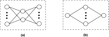
Figure 4: The extended system model. (a): The $K$ pair source nodes scenario. (b): The $T$ relay nodes scenario.

Discussion: The extended two system models are shown in Fig. 4, which are the multipair scenario with two relay nodes and $K$ pair source nodes, and the $Z$ ($Z$ should be even number) relay nodes scenario with two source nodes. In Figure 4(a), each pair sources and two relay nodes can be seen as a group. Since each pair source nodes are independent with each other, we can design that there are $K$ RFs , LFs and one CF equipped at each relay nodes. Therefor, the extended system model (a) can be seen as $K$ parallel of our proposed system model. In Figure 4(b), two source nodes and every two relay nodes can be seen as one group. Obviously, the extended system model (b) can be seen as $\frac{Z}{2}$ parallel of our proposed system model.

IV Computational Complexity Analysis

In this section, we measure the performance of the proposed QL-QR scheme in terms of the computational complexity compared with existing algorithms by using the total number of floating point operations (FLOPs). A flop is defined as a real floating operation, i.e., a real addition, multiplication, division, and so on. In [26], the authors show the computational complexity of the real Choleskey decomposition. For complex numbers, a multiplication followed by an addition needs 8 FLOPs, which leads to 4 times its real computation. According to [27], the required number of FLOPs of each matrix is described as follows:

1. Multiplication of $m\times{n}$ and $n\times{p}$ complex matrices: $8mnp-2mp$;
2. Multiplication of $m\times{n}$ and $n\times{m}$ complex matrices: $4nm\times{(m+1)}$;
3. SVD of an $m\times{n}(m\leq{n})$ complex matrix where only $\Sigma$ is obtained: $32(mn^{2}-n^{3}/3)$;
4. SVD of an $m\times{n}(m\leq{n})$ complex matrix where only $\Sigma$ and $\Lambda$ are obtained: $32(nm^{2}+2m^{3})$,
5. SVD of an $m\times{n}(m\leq{n})$ complex matrix where $U$,$\Sigma$, and $\Lambda$ are obtained: $8(4n^{2}m+8nm^{2}+9m^{3})$;
6. Inversion of an $m\times{m}$ real matrix using Gauss-Jordan elimination: $2m^{3}-2m^{2}+m$;
7. Cholesky factorization of an $m\times{m}$ complex matrix: $8m^{3}/3$.
8. QR or QL decomposition of an $m\times n$ conplex matrix $16\left(n^{2}m-nm^{2}+\frac{1}{3}m^{3}\right)$.

For the conventional RBD method [28], the authors consider a linear MU-MIMO precoding scheme for DL MIMO systems. For the non-regenerative MIMO relay systems [29], the authors investigate a precoding design for a 3-node MIMO relay network. In [2], a relay-aided system based on a quasi-EVD channel is proposed. We compare the required number of FOLPs of our proposed method with conventional precoding algorithm, such as the conventional RBD, the non-regenerative MIMO relay system, and the CD-BD algorithm as shown in Tables I, II, III, and IV, respectively, under the assumption that $N_{T}=N_{R}$ and $\overline{N}_{i}=N_{T}-N_{i}$.

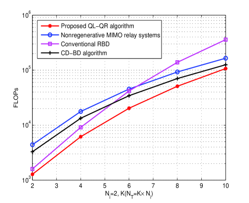
Figure 5: The complexity comparisons for required FLOPs versus the number of the users $K$.

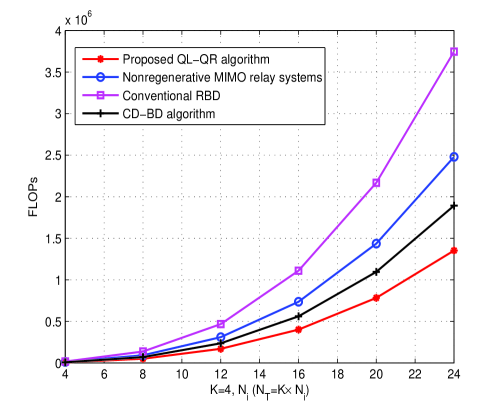
Figure 6: The complexity comparisons for required FLOPs versus the number of the receive antennas $N_{i}$ for each user.

For instance, the $(2,2,2)\times 6$ case denotes a system with three users $(K=3)$, where each user is equipped with two antennas $(N_{i}=2)$ and the total number of transmit antennas is six $(N_{T}=2\times 3=6)$. The required number FLOPs of the QL-QR algorithm, the conventional RBD, the non-regenerative MIMO relay system, and the CD-BD algorithm are counted as 33530, 40824, 45306, 34638, respectively. From these results, we can see that the reduction in the number of FLOPs of our proposed precoding method is $17.87\%$, $25.99\%$, and $3.20\%$ on an individual basis compared to the conventional RBD, the non-regenerative MIMO relay systems, and the CD-BD algorithm. Thus, our proposed QL-QR algorithm exhibits lower complexity than conventional algorithms. In addition, the complexity reduces as $N_{i}$ and $N_{T}$ increase with fixed $K$.

We summarize our calculation results of the required number of FLOPs of the alternative methods in Tables I, II, III, and IV and show them in Figures 5 and 6. Figure 5 shows the computational complexity where $N_{i}=2$ and a value of $K$ varies. And Figure 6 shows the computational complexity where $K=4$ and a value of $N_{i}$ varies. For the conventional RBD method, the orthogonal complementary vector $\mathbf{V}_{k,0}$ requires $K$ times SVD operations. If only $\mathbf{V}_{k,0}$ is obtained, it is not computationally efficient. In step 5, the efficient channel $\mathbf{H}_{eff}=\mathbf{H}_{i}\mathbf{P}^{a}_{i}$ is decomposed by the SVD with a dimension $\mathbf{R}_{eff}\times N_{T}$, where $\mathbf{R}_{eff}$ is the rank of $\mathbf{H}_{eff}$. In the nonregenerative MIMO relay method and the CD-BD algorithm, two SVD operations are performed for the channels from the source to relay and from relay to the destination, and then the efficient channel covariance matrix is measured. In the nonregenerative MIMO relay method, the authors compute $\mathbf{A}$ using the EVD an then they diagonalize $\mathbf{G}$. In the CD-BD algorithm, the authors calculate $\mathbf{V}^{a}_{i}$ by the SVD of $\mathbf{H}^{{\dagger}}_{mse}$ and then they structure $\mathbf{V}^{b}_{i}$ by using the Choleskey decomposition.

In our proposed QL-QR algorithm, we take advantage of QL and QR decompositions instead of the SVD operation, and then we compute an efficient channel as well as decompose a noise covariance matrix by the Choleskey decomposition. Finally, we calculate the determinant of $\mathbf{B}^{2}_{i}$ to solve an optimization problem. Obviously, our proposed QL-QR algorithm outperforms conventional algorithms in the light of the computational complexity.

TABLE I: Computational complexity of the proposed QL-QR Algorithm.

Step	Operations	FLOPS	Case: $(2,2,2)\times 6$
1	$\mathbf{V}_{1},\mathbf{V}_{2}$	$2\times K(40N^{3}_{i}-24N^{2}_{i}+17N_{i})$	1560
2	$\mathbf{Q}_{L,1}\mathbf{L}_{1},\mathbf{Q}_{L,2}\mathbf{L}_{2}$	$2\times 16K(N^{2}_{T}N_{i}-N_{T}N^{2}_{i}+\frac{1}{3}N^{3}_{i})$	4864
3	$\mathbf{Q}_{R,1}\mathbf{R}_{1},\mathbf{Q}_{R,2}\mathbf{R}_{2}$	$2\times 16K(N^{2}_{T}N_{i}-N_{T}N^{2}_{i}+\frac{1}{3}N^{3}_{i})$	4864
4	$\mathbf{H}^{T}_{1,1}\mathbf{F}_{1}\mathbf{H}_{1,2}$	$8N^{2}_{T}N_{i}+4N_{T}N^{2}_{i}+2N_{T}N_{i}$	696
5	$\mathbf{H}^{T}_{2,1}\mathbf{F}_{2}\mathbf{H}_{2,2}$	$8N^{2}_{T}N_{i}+4N_{T}N^{2}_{i}+2N_{T}N_{i}$	696
6	$\mathbf{\widehat{C}}_{1}$	$2K(32N^{2}_{T}N_{i}+8N_{T}N_{i}+2N^{2}_{T}-4N_{i}+3N_{T})$	14856
7	$(\mathbf{\Xi}^{H}_{i}\mathbf{\Xi}_{i})^{-1}$	$K(\frac{14}{3}N^{3}_{T}-2N^{2}_{T}+N_{T})$	2826
8	$\mathrm{det}\mathbf{B}^{2}_{1}$	$4K(N^{3}_{T}+N^{2}_{T}+2N_{T})$	3168
Total			33530

TABLE II: Computational complexity of the nonregenerative MIMO relay system [29].

Step	Operations	FLOPS	Case: $(2,2,2)\times 6$
1	$\mathbf{U}^{a}_{i}\mathbf{\Sigma}^{a}_{i}\mathbf{\Lambda}^{aH}_{i}$	$8K(4N^{2}_{T}N_{i}+8N_{T}N^{2}_{i}+9N^{3}_{i})$	13248
2	$\mathbf{U}^{a}_{j}\mathbf{\Sigma}^{a}_{j}\mathbf{\Lambda}^{aH}_{i}$	$8K(4N^{2}_{T}N_{i}+8N_{T}N^{2}_{i}+9N^{3}_{i})$	13248
3	$\mathbf{H}^{H}_{i}\mathbf{H}_{i}$	$4KN_{i}N_{T}(N_{i}+1)$	432
4	$\mathbf{H}^{H}_{j}\mathbf{H}_{j}$	$4KN_{i}N_{T}(N_{i}+1)$	432
5	$\mathbf{H}^{H}_{i}[\sigma^{2}_{1}\sigma^{2}_{2}(\mathbf{H}_{j}\mathbf{F})^{H}\mathbf{H}_{j}\mathbf{F}+\mathbf{I}]^{-1}\mathbf{H}_{i}$	$2K(N^{3}_{i}+8N_{i}N^{2}_{T}+4N^{2}_{i}N_{T}+2N_{i}N_{T}-N^{2}_{i}+N_{i})$	4212
6	$\mathbf{V}_{A}\mathbf{\Lambda}_{A}\mathbf{V}^{H}_{A}$	$8K(4N^{2}_{T}N_{i}+8N_{T}N^{2}_{i}+9N^{3}_{i}+\frac{1}{2}N_{i})$	13272
7	$\mathrm{diag}(\widetilde{\mathbf{G}})$	$K[4N_{i}N_{T}(N_{i}+1)+2N^{3}_{i}-2N^{2}_{i}+N_{i}]$	462
Total			45306

TABLE III: Computational complexity of the conventional RBD [28].

Step	Operations	FLOPS	Case: $(2,2,2)\times 6$
1	$\mathbf{U}^{a}_{i}\mathbf{\Sigma}^{a}_{i}\mathbf{\Lambda}^{aH}_{i}$	$32K(N_{T}\overline{N}^{2}_{i}+2\overline{N}^{3}_{i})$	21504
2	$\left((\mathbf{\Sigma}^{a}_{i})^{T}\mathbf{\Sigma}^{a}_{i}+\rho^{2}\mathbf{I}\right)^{-1/2}$	$K(18N_{T}N^{2}_{i}-2N^{2}_{i})$	336
3	$\mathbf{V}^{a}_{i}\mathbf{D}^{a}_{i}$	$8KN^{3}_{T}$	5184
4	$\mathbf{H}_{i}\mathbf{P}^{a}_{i}$	$K(8N_{T}N^{2}_{i}-2N^{2}_{i})$	552
5	$\mathbf{U}^{b}_{i}\mathbf{\Sigma}^{b}_{i}\mathbf{V}^{bH}_{i}$	$64K(\frac{9}{8}N^{3}_{i}+N_{T}N^{2}_{i}+\frac{1}{2}N^{2}_{T}N_{i})$	13248
Total			40824

TABLE IV: Computational complexity of the CD-BD algorithm [2].

Step	Operations	FLOPS	Case: $(2,2,2)\times 6$
1	$\mathbf{U}^{H}_{i,1}\mathbf{\Sigma}_{i,1}\mathbf{\Lambda}_{i,1}$	$8K(4N^{2}_{T}N_{i}+8N_{T}N^{2}_{i}+9N^{3}_{i})$	13248
2	$\mathbf{\Lambda}^{H}_{i,2}\mathbf{\Sigma}_{i,2}\mathbf{U}_{i,2}$	$8K(4N^{2}_{T}N_{i}+8N_{T}N^{2}_{i}+9N^{3}_{i})$	13248
3	$\mathbf{H}_{i,2}\mathbf{W}\mathbf{H}_{i,1}$	$K[8N_{i}N^{2}_{T}-2N_{i}N_{T}+4N_{i}N_{T}\times(N_{i}+1)]$	2088
4	$\mathbf{L}^{H}_{i}\mathbf{L}_{i}$	$2K(N_{i}+2N_{T}N_{i}\times(N_{i}+1)+4N^{3}_{i}/3)$	508
5	$\mathbf{H}^{{\dagger}}_{mse}$	$4N^{3}_{R}/3+12N^{2}_{R}N_{T}-2N^{2}_{R}-2N_{T}N_{R}$	2736
6	$\mathbf{H}_{i,i}\mathbf{V}^{a}_{i}\mathbf{V}^{b}_{i}$	$8K[4N_{T}N^{2}_{i}-4N^{3}_{i}/3+N^{2}_{i}(N_{i}+1)]$	2336
7	$(\mathbf{Q}_{i}\mathbf{Q}^{H}_{i}+\sigma^{2}_{i}\Psi_{i})^{-1}$	$K[4N_{R}N_{i}\times(N_{i}+1)+3N_{i}+2N^{3}_{i}-2N^{2}_{i}]$	474
Total			34638

V Simulation Results

In this section, we study the performance of the proposed QL-QR algorithm for two-way MIMO relay networks. All the simulations are performed on the assumption that all the channels are the Rayleigh fading channel and they are independently generated following $\sim{CN(0,1)}$. The noise variances $\sigma^{2}_{i}$ are equally given as $\sigma^{2}$. The total relay power constraint can be written as

$$P_{R_{1}}+P_{R_{2}}=aP_{R}+(1-a)P_{R}=P_{R},$$ (77)

where $a\in[0,1]$ is an auxiliary value as well as a power allocation coefficient between two relay nodes. All the simulation results are averaged over 1000 channel trials.

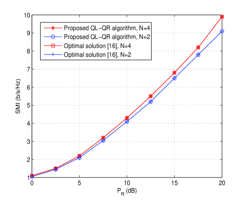
Figure 7: The achieved SMI for $N=4,2$.

In Fig. 7, we compare the sum mutual information (SMI) of various MU-MIMO schemes where full CSI is known at each node. We set $P_{1}=P_{2}=10~{}\mathrm{dB}$, $M=1$, and an equal power budget for the two relays ($a=0.5$ is assumed). The negative SMI is adopted in [16] which can be defined as

$$\mathbf{MI}_{sum}=\mathrm{log}_{2}\left|\mathbf{MSE}_{1}\right|+\mathrm{log}_{2}\left|\mathbf{MSE}_{2}\right|.$$ (78)

In our proposed method, the SMI shown in the simulation results is calculated as $-2~{}\mathrm{log}_{2}|\mathbf{B}^{2}_{i}|$ by using (55), (70), and (71). It can be observed that the proposed QL-QR algorithm has the same SMI performance as an optimal solution in [16].

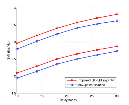
Figure 8: The SMI versus the number of the relays $T$.

Figure 8 shows the performance of our proposed SMI performance versus the number of the relays, $T$ which is even. We consider a practical scenario with different relay power constraints. We set $P_{R}=30~{}\mathrm{dB}$ and $a=0.5$. It is clear that, for different values of $P_{1}$ and $P_{2}$, a solution of our proposed QL-QR algorithm shows better performance than a max-power solution.

Figure 9 exhibits the BER performance of the BD water filling, the RBD, the SVD-RBD, and our proposed QL-QR method, where the QPSK modulation is made use of. As pointed out in [31], the BER performance for a MIMO precoding system is actually determined by the energy of the transmitted signal. To simplify our discussion, we assume $a=0$. In the RBD, $\mathrm{det}\left(\overline{\mathbf{H}}\overline{\mathbf{H}}^{H}\right)=\prod^{m}_{i=1}\lambda^{2}_{i}$, where $\overline{\mathbf{H}}\in{\mathbb{C}^{N\times M}}$, for $M<N$, is an equivalent channel matrix with its eigenvalues $\lambda_{i}$. In our proposed QL-QR method, for source node $\mathbf{S}_{1}$, we have $\mathrm{det}\left(\mathbf{\widehat{H}}_{1}\mathbf{\widehat{H}}^{H}_{1}\right)=\prod^{m}_{i=1}\varsigma^{2}_{1}$. Under the stipulaton that $\mathrm{det}\mathbf{F}_{D,i}=1$, we are able to easily obtain $\lambda_{i}=\varsigma_{1}$. Therefore, our proposed QL-QR method has the same BER performance as the SVD-RBD method.

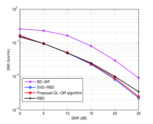
Figure 9: BER performance on the Rayleigh fading channel .

VI Conclusions

This paper studies joint optimization problem of an AF based on the MIMO TWRC, where two source nodes exchange their messages with two relay nodes. A relay filter has been designed, which is able to efficiently join the source and the relay nodes. Our main contribution is that the optimal beamforming vectors can efficiently be computed using determinant maximization techniques through an iterative QL-QR algorithm based on a MSE balancing method. Our proposed QL-QR algorithm can significantly reduce the computational complexity and has the equivalent BER performance to the SVD-BD algorithm.

References

- [1] J. N. Laneman, D. N. C. Tse, and G. W. Wornell, Cooperative diversity in wireless networks: Efficient protocols and outage behavior, IEEE Trans. Inf. Theory, vol. 50, no. 12, pp. 3062 C3080, Dec. 2004.
- [2] Wei Duan, Wei Song, Sang Seob Song, and Moon Ho Lee, ”Precoding Method Interference Management for Quasi-EVD Channel,” The Scientific World Journal, 28th. Aug. 2014.
- [3] T. M. Cover and A. A. E. Gamal, Capacity theorems for the relay channel, IEEE Trans. Inf. Theory, vol. 25, no. 5, pp. 572 C584, Sep. 1979.
- [4] Zhongyuan Zhao, Mugen Peng, Zhiguo Ding, Wenbo Wang, Hsiao-Hwa Chen, ”Denoise-and-Forward Network Coding for Two-Way Relay MIMO Systems,” IEEE Trans. Veh. Technol., vol. 63, no. 2, pp. 775-788, Feb. 2014.
- [5] Sebastien Simoens, Olga Munoz-Medina, Josep Vidal, Aitor Del Coso, ”Compress-and-Forward Cooperative MIMO Relaying With Full Channel State Information,” IEEE Trans. Signal Pross., vol. 58, no. 2, pp. 781-791, Feb. 2010.
- [6] B. Rankov and A. Wittneben, Spectral efficient protocols for halfduplex fading relay channels,” IEEE J. Sel. Areas Commun., vol. 25, no. 2, pp. 379-389, Feb. 2007.
- [7] T. Koike-Akino, P. Popovski, and V. Tarokh, Optimized constellations for two-way wireless relaying with physical network coding, IEEE J. Sel. Areas Commun., vol. 27, no. 5, pp. 773 C787, Jun. 2009.
- [8] S. Xu and Y. Hua, Optimal design of spatial source-and-relay matrices for a non-regenerative two-way MIMO relay system, IEEE Trans. Wireless Commun., vol. 5, no. 10, pp. 1645 C1655, May 2011.
- [9] Y. Rong, Joint source and relay optimization for two-way linear nonregenerative MIMO relay communications, IEEE Trans. Signal Process., vol. 60, no. 12, pp. 6533 C6546, Dec. 2012.
- [10] K.-J. Lee, H. Sung, E. Park, and I. Lee, Joint optimization for one and two-way MIMOAFmultiple-relay systems, IEEE Trans.Wireless Commun., vol. 9, no. 12, pp. 3671 C3681, Dec. 2010.
- [11] H. Bolcskei, R. U. Nabar, O. Oyman, and A. J. Paulraj, Capacity scaling laws in MIMO relay networks,” IEEE Trans. Wireless Commun., vol. 5, no. 6, pp. 1433-1444, June 2006.
- [12] K.-J. Lee, K. W. Lee, H. Sung, and I. Lee, Sum-rate maximization for two-way MIMO amplify-and-forward relaying systems,” in Proc. IEEE Veh. Technol. Conf., pp. 1-5, Apr. 2009.
- [13] F. Roemer and M. Haardt, Algebraic norm-maximizing (ANOMAX) transmit strategy for two-way relaying with MIMO amplify and forward relays, IEEE Signal Process. Lett., vol. 16, no. 10, pp. 909 C912, Oct. 2009.
- [14] T. Unger and A. Klein, Duplex schemes in multiple antenna two-hop relaying, EURASIP Journal on Advances in Signal Processing, vol. 2008,Article ID 128592, 2008.
- [15] N. Jindal and Z. Luo, Capacity limits of multiple antenna multicast, in Proceedings of the IEEE International Symposium on Information Theory (ISIT 06), pp. 1841 C1845, Seattle,Wash, USA, July 2006.
- [16] R. Zhang, Y.-C. Liang, C. C. Chai, and S. Cui, Optimal beamforming for two-way multi-antenna relay channel with analogue network coding, IEEE Journal on Selected Areas in Communications, vol. 27, no. 5, pp. 699 C712, 2009.
- [17] R. Wang and M. Tao, Joint source and relay precoding designs for MIMO two-way relaying based on MSE criterion, IEEE. Trans. Signal Process., vol. 60, no. 3, pp. 1352 C1365, Mar. 2012.
- [18] H. Wang, L. Li, L. Song, and X. Gao, A linear precoding scheme for downlink multiuser MIMO precoding systems, IEEE Commun. Lett., vol. 15, no. 6, pp. 653 C655, June 2011.
- [19] H. Park, H. J. Yang, J. Chun and R. Adve, A closed-form power allocation and signal alignment for a diagonalized MIMO two-way relay channel with linear receivers, IEEE Trans. Signal Process., vol. 60, no. 11, pp. 5948-5962, Nov. 2012.
- [20] Veria Havary-Nassab, Shahram Shahbazpanahi and Ali Grami, ”Optimal Distributed Beamforming for Two-Way Relay Networks,” IEEE Trans. Signal Process., vol. 58, no. 3, pp. 1238-1250, Mar. 2010.
- [21] Pramod Viswanath, Venkat Anantharam and David N. C. Tse, ”Optimal Sequences, Power Control, and User Capacity of Synchronous CDMA Systems with Linear MMSE Multiuser Receivers,” IEEE Trans. Inf. Theory, vol. 45, no. 6, pp. 1968 C1983, 1999.
- [22] Rui Zhang, Ying-Chang Liang, Chin Choy Chai and Shuguang Cui, ” Optimal Beamforming for Two-Way Multi-Antenna Relay Channel with Analogue Network Coding,” IEEE J. Sel. Areas Commun., vol. 27, no. 5, pp. 699 - 712, June 2009
- [23] Cristian Lameiro, Javier V a and Ignacio Santamar a, ”Amplify-and-Forward Strategies in the Two-Way Relay Channel With Analog Tx CRx Beamforming,” IEEE Trans. Veh. Technol., vol. 62, no.2, pp. 642-654, Feb. 2013.
- [24] Yue Rong, ”Simplified Algorithms for Optimizing Multiuser Multi-Hop MIMO Relay Systems,” IEEE Trans. Commun. vol. 59, no. 10, pp. 2896-2904, Oct. 2011.
- [25] S. Boyd and L. Vandenberghe, Convex Optimization. Cambridge, U.K.: Cambridge Univ. Press, 2004.
- [26] X. Gao, L. Li, P. Zhang, L. Song, G. Zhang, Q. Wang and H. Tian, ”Low-complexity RBD precoding method for downlink of multi-user MIMO system,” Electronics Letters, wol. 46, no. 23, pp. 1574 - 1576, Nov. 2010.
- [27] G. H. Golub and C. F. Van Loan, Matrix Computations, Johns Hopkins Studies in the Mathematical Sciences, Johns Hopkins University Press, Baltimore, Md, USA, 3rd edition, 1996.
- [28] H. Wang, L. Li, L. Song, and X. Gao, A linear precoding scheme for downlink multiuser mimo precoding systems, IEEE Communications Letters, vol. 15, no. 6, pp. 653 C655, 2011.
- [29] R. Mo and Y. H. Chew, Precoder design for non-regenerative MIMO relay systems, IEEE Transactions on Wireless Communications, vol. 8, no. 10, pp. 5041 C5049, 2009.
- [30] S. Vishwanath, N. Jindal, and A. Goldsmith, On the capacity of multiple input multiple output broadcast channels, in Proceedings of the International Conference on Communications (ICC 02), pp. 1444 C1450, May 2002.
- [31] C. B. Peel, B. M. Hochwald, and A. L. Swindlehurst, A vectorperturbation technique for near capacity multiantenna multiuser communication part I: channel inversion and regularization, IEEE Trans. Commun., vol. 52, no. 1, pp. 195 202, Jan. 2005.