Strong non-linearity-induced correlations for counter-propagating photons scattering on a two-level emitter

Abstract

We analytically treat the scattering of two counter-propagating photons on a two-level emitter embedded in an optical waveguide. We find that the non-linearity of the emitter can give rise to significant pulse-dependent directional correlations in the scattered photonic state, which could be quantified via a reduction in coincident clicks in a Hong-Ou-Mandel measurement setup, analogous to a linear beam splitter. Changes to the spectra and phase of the scattered photons, however, would lead to reduced interference with other photons when implemented in a larger optical circuit. We introduce suitable fidelity measures which account for these changes, and find that high values can still be achieved even when accounting for all properties of the scattered photonic state.

The realization of on-chip all-optical information processing requires the implementation of quantum computation schemes in integrated photonic circuits Matthews et al. (2009); Bruck et al. (2015); Shadbolt et al. (2012), where the information is encoded in the travelling photons Cirac et al. (1997); Kimble (2008). These schemes demand efficient single-photon sources Claudon et al. (2010); Chang et al. (2006); Santori et al. (2002), photon detectors Knill et al. (2001); O’Brien et al. (2009), and photon gates Duan and Kimble (2004); Tiecke et al. (2014). Since photons do not inherently interact, in order to realize two-photon gates such as the controlled phase or the CNOT gate O’Brien et al. (2003, 2009); Zheng et al. (2013), optical non-linearities or post selection schemes are required. As Kerr-type non-linearities are usually weak in the few-photon limit, promising candidates to mediate the two-photon interactions are quantum mechanical two-level-systems. When two photons scatter off a two-level system, non-trivial correlations can be induced in the scattered state Nysteen et al. (2015); Fan et al. (2010); Zheng et al. (2010); Baragiola et al. (2012); Roulet et al. (2014); Valente et al. (2012a), the nature of which ultimately determines the feasibility and scalability of optical circuits based on these components. Thus, a two-level-system embedded in a one-dimensional waveguide constitutes an important prototypical system in which to investigate few-photon scattering and non-linearity-induced photonic correlations. We note that such systems have been experimentally realized, for example, by self-assembled semiconductor quantum dots in photonic crystal waveguides, with emitter–waveguide coupling efficiencies reaching values in excess of 98% Arcari et al. (2014).

For two photons scattering on a single emitter, it is known that non-linearities are strongest when the photons are identical, and their spectral linewidths are comparable to that of the emitter, which results in the strongest correlations in the scattered photonic state Nysteen et al. (2015); Roulet et al. (2014). As such, identical input photons of a specific spectral lineshape are required. In the single photon case, however, it is know that such finite-width photons experience changes in both their spectra and phase as a result of the scattering process Chen et al. (2011); Fan et al. (2010), which is also known to be the case for two-photon scattering Nysteen et al. (2015). Thus, once a photon has passed through an optical gate, it is no longer identical to an input photon, which in turn may limit the effectiveness of subsequent gates. This raises questions regarding the feasibility of integrating a large number of photonic gates needed to create complex optical circuits. The purpose of this work is to explore how two-photon pulses are altered by the scattering process, and investigate how these alterations depend on the level of induced non-linearities. Interestingly, we find that non-linearaties can actually suppress spectral and phase changes, thereby increasing the similarity of the scattered and input photons. As such, even when correctly accounting for all properties of the scattered photonic state, fidelities between the scattered and a desired directionally entangled state as high as $80\%$ can still be achieved.

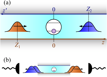
Figure 1: (a) Two counter-propagating single-photon pulses propagate toward a two-level system in its ground state. (b) The post-scattering state is measured by detectors in each chiral waveguide mode sub-group.

Various methods have been used to analyze multi-photon scattering in systems consisting of a localized scattering object coupled to a waveguide. These include fully numerical approaches Nysteen et al. (2015); Moeferdt et al. (2013), as well as analytic approaches such as the input-output formalism Fan et al. (2010), the real-space Bethe ansatz Shen and Fan (2007), the Lehmann-Symanzik-Zimmermann formalism Shi et al. (2011), Laplace transforms Huang et al. (2013), a wavefunction-based approach Valente et al. (2012a, b), and master equation formalisms (Baragiola et al., 2012). Several of these approaches allow for analytic determination of single- and two-photon scattering matrix elements, which directly relate the scattered state to the initial state of the system. Studies of two initially co-propagating photon pulses have been made for various scatterers coupling to waveguides, such as a single emitter Fan et al. (2010); Zheng et al. (2010), an emitter inside an optical cavitiy Shi et al. (2011); Shi and Fan (2013), and a non-linear optical cavity Liao and Law (2010).

Here we give a largely analytical description of the scattering of two counter-propagating photons impinging on a two-level emitter in a one-dimensional waveguide, as sketched in Fig. 1(a). We use the scattering matrix formalism, and analyse the strong non-linearity-induced correlations in the scattered state for various input states. In addition, we introduce fidelity measures to quantify the induced correlation in the scattered state, taking both the spectrum and phase of the scattered state into account, and discuss their experimental interpretations.

This paper is organized as follows: In Section I we introduce our model. In Section II we review the scattering of a single-photon pulse on a two-level-emitter, and introduce fidelity measures to quantify the similarity between the incoming and scattered photons. In Section III the formalism is extended to the scattering of two counter-propagating single-photon pulses, where our fidelity measures are used to analyse induced correlations and spectral changes, and how these relate to the level of non-linearities.

I General theory

We consider a quantum two-level-emitter coupled to two subsets of the modes in a one-dimensional waveguide as shown in Fig. 1, with the subsets differing by the direction of propagation. In the following we limit ourselves to lossless systems, though we note that this assumption could be relaxed by coupling our system to additional external reservoirs Shen and Fan (2009); Rephaeli and Fan (2013). Additionally, we neglect waveguide dispersion in the considered frequency interval, and we assume a localized scatterer (dipole approximation), i.e. that the scattering occurs only at a single point in space.

We describe the waveguide by two chiral mode subsets, being the right (mode index 1) and left (mode index 2) propagating modes. The corresponding Hamiltonian of the (bare) waveguide is

$$\tilde{H}_{0}=\sum_{i=1}^{2}\int_{0}^{\infty}\textrm{d}\tilde{k}\,\hbar{\omega}(\tilde{k})c_{i}^{\dagger}(\tilde{k})c_{i}(\tilde{k}),$$ (1)

where each mode in subsystem 1 and 2 is characterized by a wavevector $\smash{\tilde{k}}$, annihilation operator $\smash{c_{i}(\tilde{k})}$ and energy $\smash{\hbar{\omega}(\tilde{k})}$. In writing the Hamiltonian in this way we implicitly consider a single polarization of the waveguide modes. The Hamiltonian describing the emitter and its coupling to the waveguide is given by

$$\tilde{H}_{1}=\frac{\hbar\omega_{0}}{2}\sigma_{z}\!+\!\hbar g\sum_{i=1}^{2}\int_{0}^{\infty}\!\!\!\mathrm{d}\tilde{k}[\sigma_{+}c_{i}(\tilde{k})+\sigma_{-}c_{i}^{\dagger}(\tilde{k})]$$ (2)

where ${\omega}_{0}$ is the resonance frequency of the emitter and $g$ is its coupling strength to the waveguide, which is assumed to the frequency independent. This assumption is justified provided the linewidth of the emitter is small compared to the optical carrier frequencies of the photons. The operators $\sigma_{+}$ and $\sigma_{-}$ are the creation and annihilation operators of the emitter and $\sigma_{z}=\sigma_{+}\sigma_{-}-\sigma_{-}\sigma_{+}$.

We consider pulses having the same carrier wavevector $k_{p}$ and corresponding frequency $\omega_{p}=\omega(k_{p})$. It is therefore convenient to work in a frame rotating with this carrier frequency Fan et al. (2010). We relate the frequencies of the waveguide modes $\omega(\tilde{k})$ to their wavevectors using a Taylor expansion around $k_{p}$, giving

$$\omega(\tilde{k})\approx\omega_{p}+v_{g}(\tilde{k}-k_{p})$$ (3)

with $\smash{v_{g}=(\partial\omega/\partial\tilde{k})|_{\tilde{k}=k_{p}}}$ being the group velocity. The rotating frame is defined by the transformation $\tilde{H}\to H=U\tilde{H}U^{\dagger}+\mathrm{i}\hbar(\partial_{t}U^{\dagger})U$ with $U=\exp[\mathrm{i}\omega_{p}t(\sigma_{z}/2+\sum_{i}\int_{0}^{\infty}\mathrm{d}\tilde{k}c_{i}^{\dagger}(\tilde{k})c_{i}(\tilde{k}))]$. We find $H=H_{0}+H_{1}$ with

$$H_{0}=\hbar v_{g}\sum_{i=1}^{2}\int_{-\infty}^{\infty}\mathrm{d}k\,k\,a_{i}^{\dagger}(k)a_{i}(k),$$ (4)

where $k=\tilde{k}-k_{p}$ and we have defined the new annihilation operators $a_{i}(k)=c_{i}(k+k_{p})$. The interaction Hamiltonian is now given by

$$H_{1}=\frac{\hbar\Delta}{2}\sigma_{z}+\hbar g\sum_{i=1}^{2}\int_{-\infty}^{\infty}\!\!\mathrm{d}k[\sigma_{+}a_{i}(k)+\sigma_{-}a_{i}^{\dagger}(k)],$$ (5)

with $\Delta={\omega}_{0}-k_{p}v_{g}$ the detuning of the carrier frequency from the emitter transition frequency. We note that in obtaining Eqs. (4) and (5) we have extended the lower limits of integration from $-k_{p}$ to $-\infty$. This approximation is justified since we will be interested in pulses with wavevectors centered around $k=\tilde{k}-k_{p}=0$ and whose widths are much smaller than $k_{p}$.

II Single-photon scattering

Before we consider the scattering of two photons, we first review the single-photon scattering case and introduce the scattering matrix formalism. We consider cases for which the emitter is initially in its ground state. Following Fan et al. Fan et al. (2010), we relate the state of the system long after the scattering process to the initial state through the scattering matrix $S$. For non-linear scatterers the scattering matrix will in general be frequency dependent, and for a localized scatterer the scattering elements are defined as Fan et al. (2010)

$${}_{1}\langle p|S^{(1)}|k\rangle_{1}={}_{2}\langle p|S^{(1)}|k\rangle_{2}=\bar{t}_{k}\delta(p-k),$$ (6)

$${}_{2}\langle p|S^{(1)}|k\rangle_{1}={}_{1}\langle p|S^{(1)}|k\rangle_{2}=\bar{r}_{k}\delta(p-k),$$ (7)

where the notation implies, $a_{i}^{\dagger}(k)|\phi\rangle=|k\rangle_{i}$ with $|\phi\rangle$ the vacuum, and where $\bar{t}_{k}$ and $\bar{r}_{k}$ are the frequency-dependent single-photon transmission and reflection coefficients, respectively. The delta-functions reflect momentum conservation, and as no external loss channels are present, $|\bar{t}_{k}|^{2}+|\bar{r}_{k}|^{2}=1$.

An arbitrary single photon state propagating to the right is written

$$|\xi_{0}\rangle=\int_{-\infty}^{\infty}\textrm{d}k\,\xi(k)a_{1}^{\dagger}(k)|\phi\rangle,$$ (8)

where $\xi(k)$ is the wavepacket in momentum space. The post-scattering state corresponding to the incoming state expressed in Eq. (8) is defined as $|\xi\rangle_{t\to\infty}=S^{(1)}|\xi_{0}\rangle$. It is obtained by inserting the identity operator

$$\openone=\sum_{i=1,2}\int_{-\infty}^{\infty}\textrm{d}p\,|p\rangle_{i}{}_{i}\langle p|,$$ (9)

from which we find

$$|\xi\rangle_{t\rightarrow\infty}=\int_{-\infty}^{\infty}\textrm{d}p\,\bar{t}_{p}\xi(p)|p\rangle_{1}+\int_{-\infty}^{\infty}\textrm{d}p\,\bar{r}_{p}\xi(p)|p\rangle_{2}.$$ (10)

The two terms above reflect the fact that the photon can be transmitted or reflected. The scattering probabilities are defined as $P_{i}={{}_{t\rightarrow\infty}}\langle\xi|\int_{-\infty}^{\infty}\textrm{d}p\,|p\rangle_{i}{}_{i}\langle p|\xi\rangle_{t\rightarrow\infty}$, with the transmission and reflection probabilities corresponding to $i=1$ and $i=2$ respectively. These probabilities are found to be,

$$P_{1}=\int_{-\infty}^{\infty}\textrm{d}p\,|\bar{t}_{p}\xi(p)|^{2},\qquad P_{2}=\int_{-\infty}^{\infty}\textrm{d}p\,|\bar{r}_{p}\xi(p)|^{2}.$$ (11)

The theory above applies to any localized scatterer interacting with two chiral waveguide modes. We now specifically consider the emitter-waveguide system sketched in Fig. 1 and described by the Hamiltonians in Eqs. (4) and (5). In this system the reflection and transmission coefficients may be found through calculation of the single-photon scattering matrix elements Fan et al. (2010), which gives

$$\bar{t}_{k}=\frac{k-\Delta}{k-\Delta+\mathrm{i}\Gamma/(2v_{g})},\qquad\bar{r}_{k}=\frac{-\mathrm{i}\Gamma/(2v_{g})}{k-\Delta+\mathrm{i}\Gamma/(2v_{g})},$$ (12)

where $\Gamma=4\pi g^{2}/v_{g}$ is the decay rate of the emitter. We note that this form of $\Gamma$ can be found through Fermi’s Golden Rule, and is valid for a lossless system in which the emitter couples equally to modes propagating in both directions.

We consider three transform-limited incoming pulse shapes, i.e. Lorentzian, Gaussian, and step-function Gulati et al. (2014); Keller et al. (2004), which are defined by the wavepackets

$$\xi_{\text{Lor}}(k) = \frac{\sqrt{\sigma/(2\pi)}}{k-\mathrm{i}\sigma/2},$$ (13)

$$\xi_{\text{Gauss}}(k) = (\pi\sigma^{\prime 2})^{-1/4}\mathrm{e}^{-k^{2}/(2\sigma^{\prime 2})},$$ (14)

$$\xi_{\text{square}}(k) = \sigma^{-1/2}\theta(\sigma/2-|k|),$$ (15)

with $\sigma^{\prime}=(2\sqrt{\ln(2)})^{-1}\sigma$ for the Gaussian wavepacket, and where $\theta(k)$ is the Heaviside step function. All wave packets are normalised such that $\int_{-\infty}^{\infty}\textrm{d}k\,|\xi(k)|^{2}=1$, and have a spectral full width–half maximum of $\sigma$. The intensity spectra of the pulses are shown in Fig. 2 together with the spatial pulse profiles, defined as the Fourier transform $\xi(z)=(2\pi)^{-1/2}\int_{-\infty}^{\infty}\textrm{d}k\,\xi(k)\exp[\mathrm{i}kz]$.

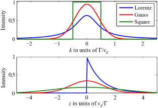
Figure 2: (a) Intensity spectra, $|\xi(k)|^{2}$, for the three single-photon wavepackets in Eqs. (13)-(15), here plotted with $\sigma=\Gamma/v_{g}$. (b) Corresponding spatial pulse profiles, $|\xi(z)|^{2}$, with large values of $z$ corresponding to the front part of the pulse, arriving first at the position of the emitter.

A comparison of the resulting reflection probabilities is shown in Fig. 3(a) for each of the three single-photon wavepackets in Eqs. (13)-(15), as has been calculated in previous works Chen et al. (2011); Zheng et al. (2010). The frequency components of the pulse closest to the transition energy of the emitter interact most strongly, and those at the exact frequency of the emitter ($k=0$) are perfectly reflected Chen et al. (2011). Thus, as the spectral pulse width is decreased, the reflection probability increases, and reaches unity for resonant monochromatic pulses ($\sigma\to 0$). In the opposite limit of $\sigma\rightarrow\infty$, only a vanishing fraction of frequency components overlap with the spectrum of the emitter, resulting in complete transmission since the pulse does not interact with the emitter. The pulse shape also has an important impact on the reflection probability. Since the Lorentzian has the largest spread of frequency components for a given FWHM, it interacts least with the emitter and correspondingly results in the lowest reflection probability.

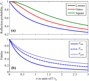
Figure 3: (a) Reflection probabilities as a function of pulse width for the three pulse shapes given in Eqs. (13)-(15) with carrier frequencies resonant with the emitter. (b) The three fidelity measures from Eqs. (17)-(21) for scattering of a Lorentzian pulse shape.

If many emitters are to be implemented in a larger sequence of photonic devices or gates, it is important that scattered photons maintain their spectral properties, i.e. the pulse shape and phase variation across the pulse. We therefore seek to define measures to compare the scattered state with some desired output state. We define three measures for this purpose, each with a different physical significance. We use the quantum state fidelity Kok and Lovett (2010) as a measure of the degree to which the scattered state is quantum mechanically identical to the desired state (neglecting overall phase differences),

$$F_{\mathrm{full}} = |\langle\xi_{\text{des}}|\xi\rangle_{t\rightarrow\infty}|^{2},$$ (16)

where $|\xi_{\mathrm{des}}\rangle$ is the desired state. When the desired state is equal to the input state but propagating in the opposite direction (i.e. a reflected but otherwise unchanged state, $|\xi_{\mathrm{des}}\rangle=\int_{-\infty}^{\infty}\xi(p)|p\rangle_{2}$), we find

$$F_{\text{full}}=\bigg{|}\int_{-\infty}^{\infty}\textrm{d}p\,\bar{r}(p)|\xi(p)|^{2}\bigg{|}^{2}.$$ (17)

This fidelity measure is appropriate, for example, if the scattered photon were to interfere with a second input photon in a Hong–Ou–Mandel-type interference experiment (where two truly indistinguishable photons exit a 50/50 beam-splitter in the same arm).

For cases in which the phase of the scattered state is unimportant, but instead we are interested in how the intensity in the pulse is distributed spectrally, the similarity between the scattered and the desired pulse may be characterized by

$$F_{\text{int}}=\left(\int_{-\infty}^{\infty}\textrm{d}p\,|\bar{r}(p)||\xi(p)|^{2}\right)^{2}.$$ (18)

This fidelity measure would be relevant when comparing the energy distributions in the scattered and desired pulse, which could be achieved by introducing spectrometers in a setup as sketched in Fig. 1(b), but disregarding the arrival times at the detectors. It can be seen to be the limiting form of a spatial definition of a fidelity measure, defined as

$$F_{\textrm{spat}}=\max_{\delta z}\bigg{|}\int_{-\infty}^{\infty}\textrm{d}z\,\xi^{*}(z)\xi_{\textrm{scat}}(z-\delta z)\bigg{|}^{2},$$ (19)

where $\xi_{\textrm{scat}}(z)$ is the spatial representation of the scattered wavepacket, which after the scattering may be displaced by $\delta z$ in the rotating frame due to a delay caused by the absorption in the emitter. Using the defined Fourier transform and Hölder’s inequality, we find $F_{\text{int}}$ is an upper bound for this spatial fidelity,

$$F_{\textrm{spat}}=\max_{\delta z}\bigg{|}\int_{-\infty}^{\infty}\textrm{d}p\,|\xi(p)|^{2}\bar{r}(p)\mathrm{e}^{\mathrm{i}\delta zk}\bigg{|}^{2}\leq F_{\text{int}}.$$ (20)

Finally, when neither the phase nor the spectral distribution are important, the scattered state may be projected onto a basis which merely counts the number of photons in each waveguide mode, e.g. as in Fig. 1(b). The fidelity in this case simply becomes the probability of detecting a photon in the desired output mode (here the reflected field),

$$F_{\text{prob}}=P_{r}.$$ (21)

We evaluate these fidelities for a Lorentzian input, and show the results in Fig. 3(b). For $F_{\textrm{full}}$ and $F_{\textrm{prob}}$ we find the exact expressions

$$F_{\text{full}} = \frac{(\tilde{\Gamma})^{2}}{(\tilde{\Gamma}+\sigma)^{2}+4\Delta^{2}},$$ (22)

$$F_{\text{prob}} = \frac{(\tilde{\Gamma}+\sigma)\tilde{\Gamma}}{(\tilde{\Gamma}+\sigma)^{2}+4\Delta^{2}},$$ (23)

where $\tilde{\Gamma}=\Gamma/v_{g}$. From Fig. 3(b) we see that $0\leq F_{\text{full}}\leq F_{\text{int}}\leq F_{\text{prob}}\leq 1$. This reflects the progressively less stringent criteria of these three measures. As the desired state in each case is a fully reflected state, the fidelities are largest for small FWHMs.

III Two-photon scattering

We now turn to the main focus of this work, and extend our formalism to describe the scattering of two-photon states. In the single-photon case, energy conservation implied that an approximately monochromatic single-photon wavepacket would scatter without changing its frequency. In the two-photon case, energy conservation only demands that the sum of the energies of the two incoming and two scattered photons is conserved. According to Fan et al. Fan et al. (2010), we can define a two-photon scattering matrix, $S^{(2)}$, in a similar way to $S^{(1)}$, which contains terms describing single-photon scattering, and also additional terms stemming from two-photon scattering processes. The additional terms involve four-wave mixing mechanisms between the two incoming and two scattered photons Fan et al. (2010); Nysteen et al. (2015).

In the rotating frame, a general two-photon state in the momentum representation is written

$$|\beta\rangle=\textstyle{\frac{1}{\sqrt{2}}} \int_{-\infty}^{\infty}\textrm{d}k\,\int_{-\infty}^{\infty}\textrm{d}k^{\prime}\,\beta_{11}(k,k^{\prime})a_{1}^{\dagger}(k)a_{1}^{\dagger}(k^{\prime})|\phi\rangle$$

$$+\textstyle{\frac{1}{\sqrt{2}}} \int_{-\infty}^{\infty}\textrm{d}k\,\int_{-\infty}^{\infty}\textrm{d}k^{\prime}\,\beta_{22}(k,k^{\prime})a_{2}^{\dagger}(k)a_{2}^{\dagger}(k^{\prime})|\phi\rangle$$

$$+ \int_{-\infty}^{\infty}\textrm{d}k\,\int_{-\infty}^{\infty}\textrm{d}k^{\prime}\,\beta_{12}(k,k^{\prime})a_{1}^{\dagger}(k)a_{2}^{\dagger}(k^{\prime})|\phi\rangle,$$ (24)

normalized such that $\int_{-\infty}^{\infty}\textrm{d}k\,\int_{-\infty}^{\infty}\textrm{d}k^{\prime}\,(|\beta_{11}(k,k^{\prime})|^{2}+|\beta_{12}(k,k^{\prime})|^{2}+|\beta_{22}(k,k^{\prime})|^{2})=1$. Introducing the notation $|kk^{\prime}\rangle_{ii^{\prime}}=\left\{{}_{i^{\prime}i}\langle k^{\prime}k|\right\}^{\dagger}=a_{i}^{\dagger}(k)a_{i^{\prime}}^{\dagger}(k^{\prime})|\phi\rangle$, the two-photon scattering elements are Fan et al. (2010)

$${}_{jj^{\prime}}\langle pp^{\prime}|S^{(2)}|kk^{\prime}\rangle_{ii^{\prime}}=\alpha_{ji,k}\alpha_{j^{\prime}i^{\prime},k^{\prime}}\delta(k-p)\delta(k^{\prime}-p^{\prime})$$

$$\quad\quad\quad\quad\quad\quad\quad\quad+\alpha_{j^{\prime}i,k}\alpha_{ji^{\prime},k^{\prime}}\delta(k-p^{\prime})\delta(k^{\prime}-p)$$

$$\quad\quad\quad\quad\quad\quad\quad\quad+\textstyle{\frac{1}{4}}B_{pp^{\prime}kk^{\prime}}\delta(p+p^{\prime}-k-k^{\prime}),$$ (25)

for $i,j\in\{1,2\}$, and where

$$\alpha_{ji,k}=\begin{cases}\bar{t}_{k}&\text{if }i=j\\ \bar{r}_{k}&\text{if }i\neq j\end{cases}$$ (26)

are the single photon reflection and transmission matrix elements. Here $B_{pp^{\prime}kk^{\prime}}$ describes interactions between the two incoming and the two scattered photons, and is determined by the specific localized scatterer considered. As in the single-photon case, to find the scattered state, we insert the identity operator, which is now given by

$$\openone=\int_{-\infty}^{\infty}\textrm{d}p\,\int_{-\infty}^{\infty}\textrm{d}p^{\prime}\,$$

$$\bigg{[}\frac{1}{2}|p^{\prime}p\rangle_{11}{{}_{11}}\langle pp^{\prime}|+|p^{\prime}p\rangle_{21}{{}_{12}}\langle pp^{\prime}|+\frac{1}{2}|p^{\prime}p\rangle_{22}{{}_{22}}\langle pp^{\prime}|\bigg{]}.$$ (27)

If we assume an initial state consisting of two counter-propagating photons, $\beta_{12}$ is the only non-zero expansion coefficient in Eq. (24), which results in the post-scattering state

$$|\beta\rangle_{t\rightarrow\infty}=\int_{-\infty}^{\infty}\textrm{d}p\,\int_{-\infty}^{\infty}\textrm{d}p^{\prime}\,\bigg{\{}$$

$$\frac{1}{2} \bigg{[}(\bar{t}_{p}\bar{r}_{p^{\prime}}+\bar{r}_{p}\bar{t}_{p^{\prime}})\beta_{12}(p,p^{\prime})+\textstyle{\frac{1}{4}}b_{12}(p,p^{\prime})\bigg{]}a_{1}^{\dagger}(p)a_{1}^{\dagger}(p^{\prime})$$

$$+ \bigg{[}(\bar{r}_{p}\bar{r}_{p^{\prime}}+\bar{t}_{p}\bar{t}_{p^{\prime}})\beta_{12}(p,p^{\prime})+\frac{1}{4}b_{12}(p,p^{\prime})\bigg{]}a_{1}^{\dagger}(p)a_{2}^{\dagger}(p^{\prime})$$

$$+\frac{1}{2} \bigg{[}(\bar{t}_{p}\bar{r}_{p^{\prime}}+\bar{r}_{p}\bar{t}_{p^{\prime}})\beta_{12}(p,p^{\prime})+\frac{1}{4}b_{12}(p,p^{\prime})\bigg{]}a_{2}^{\dagger}(p)a_{2}^{\dagger}(p^{\prime})$$

$$\hskip 156.49014pt\bigg{\}}|\phi\rangle.$$ (28)

The first term in each of the three square brackets in Eq. (28) represents single photon scattering processes, where the first factor contains the appropriate combinations of transmission and reflection coefficients connecting the initial and final photon configurations. Multi-photon process are contained in the pulse-dependent contribution $b_{12}(p,p^{\prime})$, which describes processes induced by the emitter non-linearity, and is given by

$$b_{12}(p,p^{\prime})=\int_{-\infty}^{\infty}\textrm{d}k\,\beta_{12}(k,p+p^{\prime}-k)B_{pp^{\prime}k(p+p^{\prime}-k)}.$$ (29)

We define $P_{11}$ ($P_{22}$) as the probability that both photons are measured propagating in waveguide mode 1 (mode 2), and $P_{12}$ the probability that one photon propagates in each waveguide mode. From Eq. (28) we find

$$P_{11} =\frac{1}{2}\int_{-\infty}^{\infty}\textrm{d}p\,\int_{-\infty}^{\infty}\textrm{d}p^{\prime}\,$$

$$\bigg{|}(\bar{t}_{p}\bar{r}_{p^{\prime}}+\bar{r}_{p}\bar{t}_{p^{\prime}})\beta_{12}(p,p^{\prime})+\frac{1}{4}b_{12}(p,p^{\prime})\bigg{|}^{2},$$ (30)

$$P_{12} =\int_{-\infty}^{\infty}\textrm{d}p\,\int_{-\infty}^{\infty}\textrm{d}p^{\prime}\,$$

$$\bigg{|}(\bar{t}_{p}\bar{t}_{p^{\prime}}+\bar{r}_{p}\bar{r}_{p^{\prime}})\beta_{12}(p,p^{\prime})+\frac{1}{4}b_{12}(p,p^{\prime})\bigg{|}^{2},$$ (31)

with $P_{11}=P_{22}$ and $P_{11}+P_{12}+P_{22}=1$.

As in the single photon case, we will be interested in comparing the scattered two-photon state described by Eq. (28) to some desired state using the fidelity measures we have introduced in Eqs. (17)-(21). For this purpose we consider the scattered two-photon state that would be obtained if the scatterer were replaced by a perfect 50/50 beam-splitter, which preserves the shape and phase of the input photons. In this case the scattered state would be

$$|\beta_{\textrm{des}}\rangle =\frac{1}{\sqrt{2}}\int_{-\infty}^{\infty}\textrm{d}k\,\int_{-\infty}^{\infty}\textrm{d}k^{\prime}\,\beta_{12}(k,k^{\prime})$$

$$\times\bigg{[}\frac{1}{\sqrt{2}}a_{1}^{\dagger}(k)a_{1}^{\dagger}(k^{\prime})+\frac{1}{\sqrt{2}}a_{2}^{\dagger}(k)a_{2}^{\dagger}(k^{\prime})\bigg{]}|\phi\rangle.$$ (32)

With this desired state our fidelity measures become

$$\!\!F_{\text{full}} =\!\bigg{|}\!\int_{-\infty}^{\infty}\!\!\!\mathrm{d}p\int_{-\infty}^{\infty}\!\!\!\mathrm{d}p^{\prime}\beta_{12}^{*}(p,p^{\prime})\beta_{12}^{\prime}(p,p^{\prime})\bigg{|}^{2}$$ (33)

$$\!\!F_{\text{int}} =\!\bigg{[}\!\int_{-\infty}^{\infty}\!\!\!\mathrm{d}p\int_{-\infty}^{\infty}\!\!\!\mathrm{d}p^{\prime}|\beta_{12}(p,p^{\prime})|\,|\beta_{12}^{\prime}(p,p^{\prime})|\bigg{]}^{2}$$ (34)

$$F_{\text{prob}} =P_{11}+P_{22}$$ (35)

with $\beta_{12}^{\prime}(p,p^{\prime})=(\bar{t}_{p}\bar{r}_{p^{\prime}}+\bar{r}_{p}\bar{t}_{p^{\prime}})\beta_{12}(p,p^{\prime})+\frac{1}{4}b_{12}(p,p^{\prime})$.

III.1 Two-level scatterer

The theory presented above is valid for any localized scatterer. We now specifically consider the two-level-emitter–waveguide system described by Eq. (5), and focus here only on pulses starting equidistantly from the emitter. Furthermore, we only treat pairs of input pulses with the same spectral linewidth, although the formalism can be straightforwardly extended to more general cases. For a two-level-emitter the single photon transmission and reflection matrix elements $\bar{t}_{k}$ and $\bar{r}_{k}$ are given by Eq. (12), while the two-photon scattering element is Fan et al. (2010)

$$B_{pp^{\prime}kk^{\prime}}=\mathrm{i}\frac{\sqrt{\Gamma}}{\pi}s_{p}s_{p^{\prime}}(s_{k}+s_{k^{\prime}}),$$ (36)

where

$$s_{k}=\frac{\sqrt{\Gamma}/v_{g}}{k-\Delta+\mathrm{i}\Gamma/(2v_{g})}.$$ (37)

We only consider uncorrelated photon input states, and as such $\beta(k,k^{\prime})$ is a symmetrized product of two single-photon wavepackets $\beta(k,k^{\prime})=[\xi(k)\xi^{\prime}(k^{\prime})+\xi^{\prime}(k)\xi(k^{\prime})]$, which is normalized as $\int_{-\infty}^{\infty}\textrm{d}k\,\int_{-\infty}^{\infty}\textrm{d}k^{\prime}\,|\beta(k,k^{\prime})|^{2}=1$.

We begin our analysis of the scattered state by considering correlations in photon detection events in the two waveguide mode subsets, as depicted in Fig. 1(b). In this case no information regarding the spectrum and phase of the scattered photons is obtained, and the appropriate fidelity measure is $F_{\text{prob}}$, which is equal to $1$ minus the probability of detecting a coincidence in the two detectors, i.e. for $F_{\text{prob}}=1$ no coincidence events are measured (a perfect Hong-Ou-Mandel dip would be observed). In Fig. 4(a), $F_{\text{prob}}$ is calculated for Gaussian and Lorentzian input pulses for zero detuning $(\Delta=0)$, for which the interaction between the pulses and emitter is greatest. We see that very high fidelities are obtained, reaching values of $\sim 80\%$ for the Lorentzian input and $\sim 90\%$ for the Gaussian. Maximal correlations are achieved in the regime where the emitter and pulse linewidth are similar, as has been demonstrated numerically in earlier work Nysteen et al. (2015). Interestingly, although the Lorentzian pulse shape is well-known to be the optimal pulse shape for maximally exciting the two-level emitter with a single photon Rephaeli et al. (2010), it is not the optimal shape for maximizing the directional correlations in the scattered state.

The high fidelities obtained demonstrate that the scattered states are highly directionally entangled, in analogy with the effect of an optical beam-splitter. However, in contrast to the classical beam splitter, the high correlation seen here is induced solely by non-linearities. To demonstrate that the high directional correlations indeed stem from non-linearities, in Fig. 4(a) we also show the case where the non-linear two-photon interaction term $b_{12}(p,p^{\prime})$ has been artificially set to $0$ (dashed curves). For an uncorrelated two-photon input pulse which is resonant with the emitter and which has a symmetric spectral wavefunction amplitude, $|\xi(-k)|^{2}=|\xi(k)|^{2}$, as is the case here, Eq. (30) reduces to

$$P_{11}=a(1-a),$$

$$\text{with }a=\int_{-\infty}^{\infty}\textrm{d}p\,\frac{(\tilde{\Gamma}/2)^{2}}{p^{2}+(\tilde{\Gamma}/2)^{2}}|\xi(p)|^{2},$$ (38)

showing that $P_{11}$ maximally attains the value $1/4$, occurs when $a=1/2$. Thus, $F_{\text{prob}}=2P_{11}$ never exceeds 1/2, as confirmed in Fig. 4(a), which indicates that no directional entanglement is present in the scattered state Kok and Lovett (2010). For $b_{12}(p,p^{\prime})=0$, the emitter behaves as a linear component (e.g. a lossless optical cavity) and cannot mediate interactions between the two photons. As such, the scattering process is determined entirely by interference effects, which, unlike an optical beam-splitter, cannot create entanglement in this system when the pulses are resonant with the emitter.

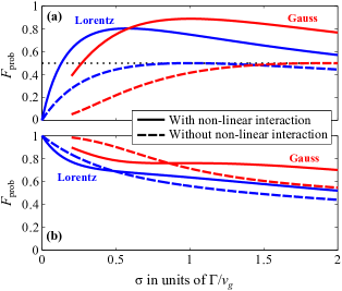
Figure 4: Degree of directional entanglement $F_{\text{prob}}$ plotted for varying incoming pulse widths, shown for both Lorentzian and Gaussian input pulses (solid lines). The corresponding values obtained when neglecting two-photon scattering terms are also shown (dashed lines). (a) Pulse and emitter are resonant, $\Delta=0$. (b) Pulse and emitter detuned by $\Delta=\Gamma/(2v_{g})$.

A more direct analogy with a 50/50 beam splitter can be obtained by detuning the input pulses by half the emitter linewidth, $\Delta=\Gamma/(2v_{g})$. For this value of the detuning, a monochromatic single-photon pulse will be reflected/transmitted with 50% probability (whereas at $\Delta=0$ a monochromatic single-photon pulse is fully reflected). Fig. 4(b) shows $F_{\mathrm{prob}}$ for $\Delta=\Gamma/(2v_{g})$, and we confirm that $F_{\mathrm{prob}}\to 1$ as $\sigma\to 0$ as expected. The change in the fidelity due to the non-linearities now becomes smaller than in the resonant case, as the interaction between the pulse and the emitter is less efficient off resonance. Interestingly, in this case, for small $\sigma$, the non-linear interaction actually deteriorates the beam splitting effect, since now the directional entanglement can be generated by interference effects only.

For a Lorentzian input analytic expressions for $P_{11,\text{Lor}}=P_{22,\text{Lor}}$ may be derived. We find

$$P_{11,\text{Lor}}=\frac{3\tilde{\Gamma}\sigma(3\sigma\!+\!\tilde{\Gamma})(\sigma\!+\!\tilde{\Gamma})+4\Delta^{2}\tilde{\Gamma}(\sigma\!+\!2\tilde{\Gamma})}{\left[(3\sigma+\tilde{\Gamma})^{2}+4\Delta^{2}\right]\left[(\sigma+\tilde{\Gamma})^{2}+4\Delta^{2}\right]}$$ (39)

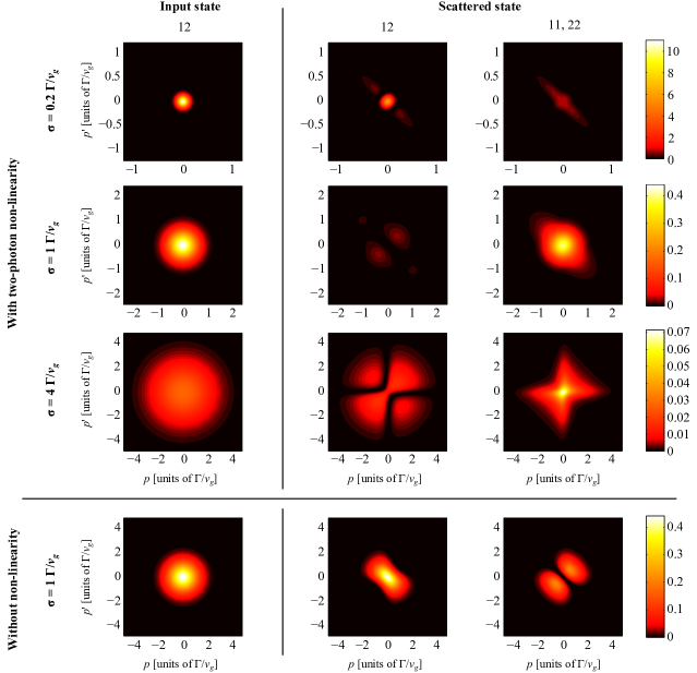
Figure 5: Intensity spectrum of an incoming Gaussian two-photon state for two counter-propagating photons (left column), and the resulting two-photon intensity spectra for the scattered state (middle and right columns) for photons scattering in different directions, 12, and where both photons propagate in the same direction, 11 (identical to 22), with $\Delta=0$. The spectral width of the input pulses is varied: $\sigma=0.2\,\tilde{\Gamma}$ (1st row), $\sigma=1\,\tilde{\Gamma}$ (2nd row), and $\sigma=4\,\tilde{\Gamma}$ (3rd row). The intensity spectra are also shown for scattering with the non-linearity turned off, $b_{12}(p,p^{\prime})=0$, using $\sigma=1\,\tilde{\Gamma}$ (4th row).

with $\tilde{\Gamma}=\Gamma/v_{g}$. The maximum value on resonance ($\Delta=0$) is obtained for $\sigma/\tilde{\Gamma}=3^{-1/2}\approx 0.57$, at which point $P_{11,\text{Lor}}\approx 0.40$ (and $F_{\mathrm{prob}}=2P_{11,\text{Lor}}\approx 0.8$), in agreement with Fig. 4(a). In comparison, with no non-linear terms, $b_{12}(p,p^{\prime})=0$, the scattering probability becomes

$$P^{\text{one}}_{11,\text{Lor}}=\frac{\sigma\tilde{\Gamma}(\sigma+\tilde{\Gamma})^{2}+4\Delta^{2}\tilde{\Gamma}(\sigma+2\tilde{\Gamma})}{\left[(\sigma+\tilde{\Gamma})^{2}+4\Delta^{2}\right]^{2}}$$ (40)

which has an on-resonance maximum for $\sigma=\tilde{\Gamma}$, giving $F_{\mathrm{prob}}=2P^{\text{one}}_{RR,\text{Lor}}=1/2$. Thus, for the Lorentzian pulse, non-linearities increase the scattering probability by a factor of $P_{11,\text{Lor}}/P^{\text{one}}_{11,\text{Lor}}=1+2/(1+3\sigma/\tilde{\Gamma})$ on resonance. For $\sigma\rightarrow\infty$, the interaction with the emitter becomes infinitely weak and no enhancement is present. In the opposite limit of $\sigma\rightarrow 0$, the enhancement factor is 3.

III.2 Scattering Fidelities

As discussed above, if the scatterer is to be implemented in a larger optical circuit, in addition to considering in which direction the photons scatter, the amplitude and phase of the different frequency components may also be important. In such a case, $F_{\text{prob}}$ is no longer a sufficient fidelity measure, since it contains only directional information. As illustrated in Fig. 5, where we plot the intensity spectrum of a scattered Gaussian wavepacket, the spectra of the scattered pulses change significantly during the scattering process. For input pulses with a narrow spectral linewidth compared to the emitter (1st row), the pulse power at the emitter position remains low due to the corresponding broad spatial profiles of the pulses. In that case, the non-linearity is only weakly addressed, and the individual photons are predominately reflected. A weak non-linearity-induced four-wave mixing process is signified by the appearance of diagonal features, as one photon achieves a larger energy, while the energy of the other decreases. When the pulse and emitter linewidths are comparable (2nd row), the predicted strong directional correlation is induced Nysteen et al. (2015), with the pulse profile being almost preserved. For spectrally broad pulses (3rd row), only the near-resonant part of the spectrum interacts with the emitter. We see that the spectral components at the emitter frequency are absent from the transmitted pulse since these have been reflected without significant two-photon effects.

Interestingly, the fact that the pulse spectrum is almost perfectly preserved when the pulse and emitter linewidths are comparable (2nd row) can be attributed to non-linearities. This can be seen in the 4th row, where we again show the initial and scattered spectra for the case $\sigma=\tilde{\Gamma}$, but where we have artificially set the non-linear term equal to zero, $b_{12}=0$. By comparison with the 2nd row, we can clearly see that the non-linearities not only give rise to the directional entanglement, but also suppress changes to the spectral shape.

To quantify both the spectral and phase deviations between the scattered and the desired state, all three fidelities defined in Eqs. (33)-(35) are shown in Fig. 6. By comparing $F_{\text{prob}}$ to $F_{\text{int}}$, i.e. taking into account the difference in the spectra of the scattered and desired pulse (but not the phase), we see that the fidelity becomes lower, and most significantly so for pulses with a small spectral linewidth. This can be understood from Fig. 5, where we see that the scattered wavepacket for the spectrally narrow input (1st row) is clearly influenced by strong four-wave mixing effects. For pulses with larger widths, these effects are weaker, since a larger fraction of frequency components are detuned from the emitter transition and therefore interact only weakly.

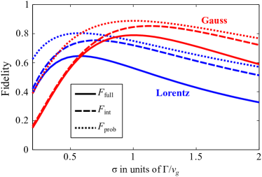
Figure 6: Fidelities from Eqs. (33)-(35) plotted for varying width of the input pulses, shown both for Gaussian and Lorentzian inputs on resonance with the emitter.

Scattering-induced phase differences across the pulses may be examined by comparison of $F_{\text{int}}$ and $F_{\text{full}}$. As illustrated in Fig. 6, these fidelities are almost equal for spectrally narrow pulses, whereas significant deviations are seen for spectrally broad pulses. This may be explained by considering the simpler single-photon scattering case. From Eq. (12), we see that a resonant, monochromatic pulse will be reflected with a phase shift of $\pi$, whereas spectrally broader pulses attain a phase shift from $\pi/2$ to $3\pi/2$ across the pulse spectrum. Thus, spectrally broad pulses experience larger decreases in the fidelity due to phase mismatching with our given desired state.

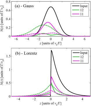
Figure 7: The photon density in the moving frame, $N(z)$, calculated for the input pulse and for photons in the same (11 identical to 22) or in different modes after the scattering (12) for resonant input pulses with $\sigma=1\,\tilde{\Gamma}$ and $\Delta=0$. The largest values of $z$ correspond to the front part of the pulse, and the solid (dashed) lines include (do not include) the non-linear two-photon interaction, $b_{12}(p,p^{\prime})$. (a) Gaussian wavepacket (b) Lorentzian wavepacket.

As the phase changes correspond to modifications to the spatial profile of the pulse, we specifically consider how the spatial pulse profile (here analogous to the temporal shape) is changed during the scattering process. To clearly illustrate the effect of the non-linear scattering on the spatial profile, we evaluate the photon density at a specific point of the photon wavepacket in the rotating frame, defined as

$$N(z)=_{t\rightarrow\infty}\langle\beta|a^{\dagger}(z)a(z)|\beta\rangle_{t\rightarrow\infty}$$ (41)

where $a(z)=(2\pi)^{-1/2}\int_{-\infty}^{\infty}\textrm{d}k\,a(k)\exp[\mathrm{i}kz]$ is the annihilation operator for an excitation at a position $z$ in a frame rotating with the pulses. For Gaussian and Lorentzian input pulses, the photon density is plotted in Fig. 7. For both pulse shapes, we see that a delay occurs due to interaction with the emitter, and furthermore the non-linearity improves the similarity between the scattered and incoming field. The Gaussian pulse is observed to preserve its spatial symmetry, as compared to the Lorentzian input pulse. This is due to the fact that the part of the photon pulses which is absorbed by the emitter is re-emitted with an exponential shape that is spatially reversed compared to the input pulse, which explains why $F_{\text{prob}}$ deviates significantly from $F_{\text{int}}$ for large spectral linewidths in Fig. 6.

IV Conclusion

We have analytically demonstrated that the non-linearity of a two-level-emitter can induce strong pulse-dependent directional correlations (entanglement) in the scattered state of two initially counter propagating photons. These correlations are maximized for photons with spectral widths comparable to that of the emitter, and also depend on the specific spectral shape of the photons. Furthermore, we have investigated how the spectra and phase of the photons are affected by the scattering process, and introduced different fidelity measures to quantify the similarity of the scattered and input photons. Interestingly, for photons with spectral widths comparable to the emitter linewidth, where the directional correlations are maximized, the non-linearity of the emitter acts to suppress changes in the spectra and phase of the photons. As such, even when taking all properties of the scattered state into account, a comparison to perfect directionally entangled photons with preserved spectra and phases gives fidelities as high as $\sim 80\%$ for Gaussian pulse shapes. A comparison of our fidelity measures indicates that when engineering photonic gate structures and other functionalities using two-level-emitters, it is important to also consider spectral and phase changes when determining the efficiency and scalability of non-linear photonic devices.

References

- Matthews et al. (2009) J. C. F. Matthews, A. Politi, A. Stefanov, and J. L. O’Brien, Nat. Photonics 3, 346 (2009).
- Bruck et al. (2015) R. Bruck, B. Mills, B. Troia, D. J. Thomson, F. Y. Gardes, Y. Hu, G. Z. Mashanovich, V. M. N. Passaro, G. T. Reed, and O. L. Muskens, Nat. Photonics 9, 54 (2015).
- Shadbolt et al. (2012) P. J. Shadbolt, V. M. R., A. Peruzzo, A. Politi, A. Laing, M. Lobino, J. C. F. Matthews, M. G. Thompson, and J. L. O’Brien, Nat. Photonics 6, 45 (2012).
- Cirac et al. (1997) J. I. Cirac, P. Zoller, H. J. Kimble, and H. Mabuchi, Phys. Rev. Lett. 78, 3221 (1997).
- Kimble (2008) H. J. Kimble, Nature 453, 1023 (2008).
- Claudon et al. (2010) J. Claudon, J. Bleuse, N. S. Malik, M. Bazin, P. Jaffrennou, N. Gregersen, C. Sauvan, P. Lalanne, and J.-M. Gerard, Nat. Photonics 4, 174 (2010).
- Chang et al. (2006) W.-H. Chang, W.-Y. Chen, H.-S. Chang, T.-P. Hsieh, J.-I. Chyi, and T.-M. Hsu, Phys. Rev. Lett. 96, 117401 (2006).
- Santori et al. (2002) C. Santori, D. Fattal, J. Vuckovic, G. S. Solomon, and Y. Yamamoto, Nature 419, 594 (2002).
- Knill et al. (2001) E. Knill, R. Laflamme, and G. J. Milburn, Nature 409, 46 (2001).
- O’Brien et al. (2009) J. L. O’Brien, A. Furusawa, and J. Vuckovic, Nat. Photonics 3, 687 (2009).
- Duan and Kimble (2004) L.-M. Duan and H. J. Kimble, Phys. Rev. Lett. 92, 127902 (2004).
- Tiecke et al. (2014) T. G. Tiecke, J. D. Thompson, N. P. de Leon, L. R. Liu, V. Vuletic, and M. D. Lukin, Nature 508, 241 (2014).
- O’Brien et al. (2003) J. L. O’Brien, G. J. Pryde, A. G. White, T. C. Ralph, and D. Branning, Nature 426, 264 (2003).
- Zheng et al. (2013) H. Zheng, D. J. Gauthier, and H. U. Baranger, Phys. Rev. Lett. 111, 090502 (2013).
- Nysteen et al. (2015) A. Nysteen, P. T. Kristensen, D. P. S. McCutcheon, P. Kaer, and J. Mørk, New J. Phys. 17, 023030 (2015).
- Fan et al. (2010) S. Fan, Ş. E. Kocabaş, and J.-T. Shen, Phys. Rev. A 82, 063821 (2010).
- Zheng et al. (2010) H. Zheng, D. J. Gauthier, and H. U. Baranger, Phys. Rev. A 82, 063816 (2010).
- Baragiola et al. (2012) B. Baragiola, R. Cook, A. Brańczyk, and J. Combes, Phys. Rev. A 86, 013811 (2012).
- Roulet et al. (2014) A. Roulet, H. N. Le, and V. Scarani, arXiv:1411.6411 (2014).
- Valente et al. (2012a) D. Valente, Y. Li, J. P. Poizat, J. M. Gérard, L. C. Kwek, M. F. Santos, and A. Auffèves, New J. Phys. 14, 083029 (2012a).
- Arcari et al. (2014) M. Arcari, I. Söllner, A. Javadi, S. L. Hansen, S. Mahmoodian, J. Liu, H. Thyrrestrup, E. H. Lee, J. D. Song, S. Stobbe, et al., Phys. Rev. Lett. 113, 093603 (2014).
- Chen et al. (2011) Y. Chen, M. Wubs, J. Mørk, and A. F. Koenderink, New Journal of Physics 13, 103010 (2011).
- Moeferdt et al. (2013) M. Moeferdt, P. Schmitteckert, and K. Busch, Opt. Lett. 38, 3693 (2013).
- Shen and Fan (2007) J.-T. Shen and S. Fan, Phys. Rev. A 76, 062709 (2007).
- Shi et al. (2011) T. Shi, S. Fan, and C. P. Sun, Phys. Rev. A 84, 063803 (2011).
- Huang et al. (2013) J.-F. Huang, J.-Q. Liao, and C. P. Sun, Phys. Rev. A 87, 023822 (2013).
- Valente et al. (2012b) D. Valente, Y. Li, J. P. Poizat, J. M. Gérard, L. C. Kwek, M. F. Santos, and A. Auffèves, Phys. Rev. A 86, 022333 (2012b).
- Shi and Fan (2013) T. Shi and S. Fan, Phys. Rev. A 87, 063818 (2013).
- Liao and Law (2010) J.-Q. Liao and C. K. Law, Phys. Rev. A 82, 053836 (2010).
- Shen and Fan (2009) J.-T. Shen and S. Fan, Phys. Rev. A 79, 023837 (2009).
- Rephaeli and Fan (2013) E. Rephaeli and S. Fan, Photonics Research 1, 110 (2013).
- Gulati et al. (2014) G. K. Gulati, B. Srivathsan, B. Chng, A. Cerè, D. Matsukevich, and C. Kurtsiefer, Phys. Rev. A 90, 033819 (2014).
- Keller et al. (2004) M. Keller, B. Lange, K. Hayasaka, W. Lange, and H. Walther, Nature 431, 1075 (2004).
- Kok and Lovett (2010) P. Kok and B. W. Lovett, Introduction to Optical Quantum Information Processing (Cambridge University Press, 2010).
- Rephaeli et al. (2010) E. Rephaeli, J.-T. Shen, and S. Fan, Phys. Rev. A 82, 033804 (2010).