Adaptive Synchronization and Anticipatory Dynamical System

Abstract

Many biological systems can sense periodical variations in a stimulus input and produce well-timed, anticipatory responses after the input is removed. Such systems show memory effects for retaining timing information in the stimulus and cannot be understood from traditional synchronization consideration of passive oscillatory systems. To understand this anticipatory phenomena, we consider oscillators built from excitable systems with the addition of an adaptive dynamics. With such systems, well-timed post-stimulus responses similar to those from experiments can be obtained. Furthermore, a well-known model of working memory is shown to possess similar anticipatory dynamics when the adaptive mechanism is identified with synaptic facilitation. The last finding suggests that this type of oscillators can be common in neuronal systems with plasticity.

The interaction between a dynamical system capable of oscillatory behavior and an external periodic stimulus input represents the fundamental physics underlying many biological and engineering systems Pikovsky and Kurths (2003); Gros (2011). Under the titles of synchronization or entrainment, active studies have been devoted to various aspects of these systems, for example, the existence and degree of synchrony under different parameter conditions, the stability of the synchronous state, the influence of noise Pikovsky and Kurths (2003), and, recently, the efficiency of entrainment Zlotnik et al. (2013). While these mostly involve how the systems enter or stay under the rhythmic interaction, the post-interaction behavior of the systems often plays important roles in many biological functions Winfree (2001). This potentially allows the biological systems to recognize the temporal patterns in the environment and produce anticipatory responses to help their survival. Examples of such transient responses following the end of stimulus have been observed in ganglion cells of retina under light stimulus Schwartz et al. (2007), growth of slime mold influenced by varying humidity Saigusa et al. (2008), and the optic tectum of zebrafish conditioned with moving periodic scenery Sumbre et al. (2008). However, the underlying physics for this time perception mechanism is still unclear and there is a ongoing debate on whether a clock is needed Bueti et al. (2010).

To explain the anticipative dynamics, it has been proposed that the periods of various lengths can be built into the structure of a network with loops of various sizes Mi et al. (2013). External stimulations of a particular period will then activate a particular circuit in the system to provide the memory effect. This implementation of “memory” with pre-fabricated structure is similar in spirit to the phase model used to understand the anticipation of slime mold Saigusa et al. (2008). In this phase model, oscillators with various periods must be first put into the system before an external stimulation of a particular frequency can be used to entrain or synchronize the oscillators with the same frequency to provide the anticipation effect. An obvious objection to this type of models of pre-fabricated structures is that a continuous change in external periods will not produce a continuous change in the response; contrary to findings of experiments with retina.

In our view, the anticipation effect is the adaptation of a biological system to a periodic stimulation. In the following, we show the function of such anticipation can be achieved by a minimal dynamical system with two-dimensional oscillations controlled by a slow adaptive dynamics. A surprisingly well retention of periodicity information for a range of stimulus period can be obtained with single parameter adjustment, and thus can be easily targeted evolutionarily. Such dynamical mechanism does not necessarily describe a dominating microscopic cellular process or pathway. It can also act as a coarse-grained, thermodynamic description for systems of many degrees of freedom. In a neural network model for working memory Mongillo et al. (2008), we show an anticipative dynamics can be produced in the mean-field level of the network with the adaptation coming from the residual calcium dynamics of synaptic facilitation. This suggests a validity test for our idea in experiments. Furthermore, our model demonstrates that the anticipative mechanism can be quite generic and may be wide spread in natural neural systems; hinting that the perception of time in biological systems does not require the existence of a clock.

To substantiate our considerations, we use a reduced FitzHugh-Nagumo (FHN) model FitzHugh (1961) defined by the equations,

$$\frac{dv}{dt}=v-\frac{v^{3}}{3}-w+I_{\text{ext}}\left(t\right),$$ (1)

$$\frac{dw}{dt}=\frac{1}{\tau}\left(v+a\right).$$ (2)

Note that we are just using the generic excitable properties of the model to demonstrate our idea. The excited state of the FHN model considered here does not represent an action potential and the time scale of the system can be much longer than the spiking dynamics typically associated with the FHN model. Usually, the system parameter $a$ is a constant for the FHN model. However, to perceive the period of a periodic stimulus input, we turn $a$ into a dynamic variable, allowing the system to adapt to different limiting behavior. It is known that the dynamics of $v$ and $w$ can be synchronized to that of the periodic $I_{\text{ext}}$ when $a$ and $\tau$ are properly chosen. The adaptation of $a$ to the external period can be written in general as:

$$\frac{da}{dt}=\frac{1}{\tau_{a}}\left(\hat{a}-a\right)$$ (3)

where $\hat{a}\equiv g\left(v,w\right)$ is the entrained value of $a$ and we assume that the adaptive process is characterized by a single time scale of relaxation much slower than the FHN dynamics ($\tau_{a}\gg\tau$). The physical meaning of such requirement is that the value of $a$ will be close to the entrained value $\hat{a}$ when there is external stimulation and will relax back to its resting value $a_{0}$ when the stimulation is removed. Anticipative dynamics will be manifested during the relaxation of $a$ from $\hat{a}$ to $a_{0}$. Our task is to find a reasonable form for $g\left(v,w\right)$ to ensure the adaptation dynamics is stable.

As adaptation is a slower process when compared to the oscillatory dynamics of the system, we expect $\left\langle\hat{a}\right\rangle$ to depend on moments of $v$ and $w$, where $\left\langle\cdot\right\rangle$ indicates time-averaged values over stationary cycles of the driven system. It can be shown that since $\left\langle v\right\rangle=-\left\langle a\right\rangle$ and $\left\langle w\right\rangle=\left\langle v\right\rangle-\frac{1}{3}\left\langle v^{3}\right\rangle+\left\langle I_{\text{ext}}\left(t\right)\right\rangle$, only $\left\langle w\right\rangle$ contains significant information of $I_{\text{ext}}$. Thus, to the lowest order, the function $g\left(v,w\right)$ is of the form

$$g=a_{c}-pw$$ (4)

where $a_{c}$ and $p$ are constant parameters that need to be tuned for the best behavior. To maintain a stable fixed point at $a=a_{0}>1$ under the adaptation dynamic (3), in the absence of external stimulus, the parameters in Eq. (4) should satisfy

$$a_{c}=\left(1-p\right)a_{0}+p\frac{a_{0}^{3}}{3}.$$ (5)

For a more intuitive view of the phase space, we will use $p$ and $a_{0}$ as the control parameters for the adaptive dynamics.

A

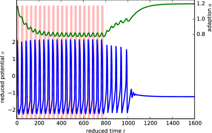
B

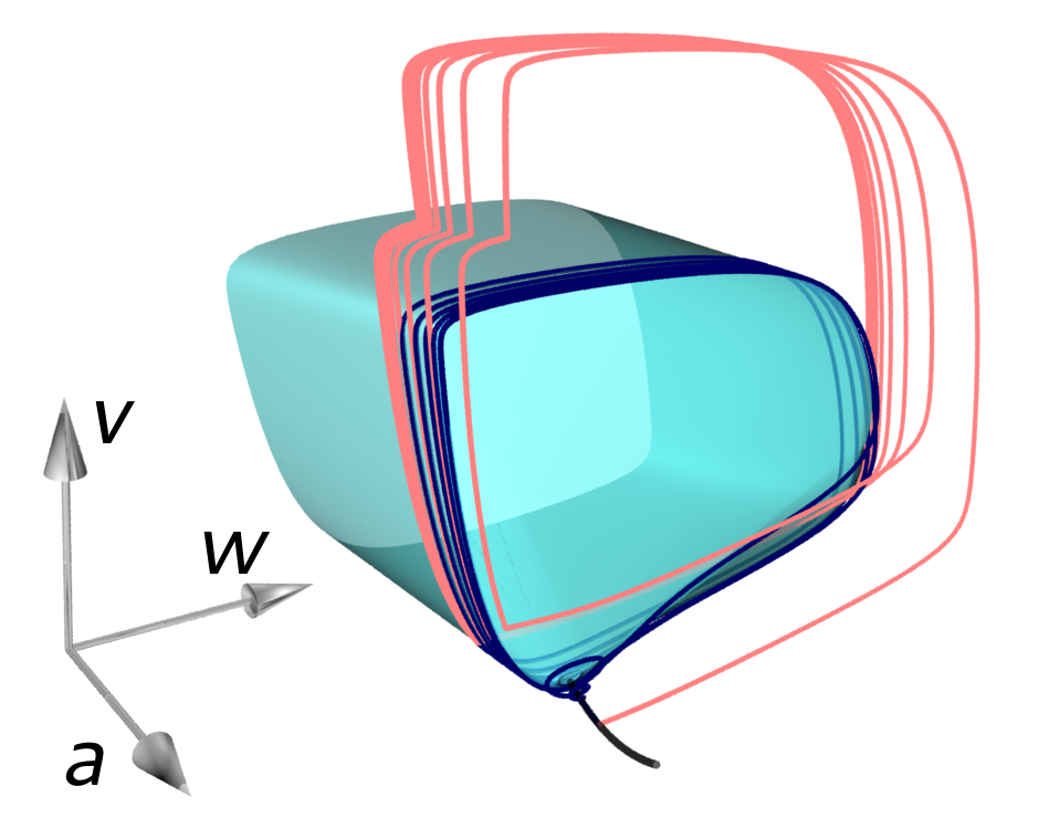
Figure 1: (Color online) A. Sustained oscillations of a stimulus-induced, adaptive oscillator. The square-wave stimulus (shaded area) lasting for 20 cycles has an amplitude of 1, periods of 40, and duty ratio of $1/2$. The control parameters for the adaptive dynamics are $a_{0}=1.2$ and $p=0.3$. B. State space trajectory for the same process when the system is driven from the fixed point (red/light curve) and when it relaxes back to the fixed point (blue/dark curve). The attractor manifold of the system (cyan/shaded surface) is constructed from the limit cycles of the simplified FitzHugh-Nagumo for fixed $a<1$ values. The black line attached to the manifold consists of the fixed points for $a\geq 1$.

Figure 1 shows the response of our adaptive model to a transient periodic stimulation ($T_{s}=40$) with $p=0.3$, $a_{0}=1.2$. Here, for convenience, we have used a dimensionless time with constants $\tau=10$, and $\tau_{a}=100$. It can be seen in Fig. 1A that the parameter $a$ starts from its resting value of 1.2 and decreases to a mean value of $\left\langle\hat{a}\right\rangle\approx 0.8$ as the stimulus $I_{\text{ext}}$ is applied and entrains the dynamics of $v$ and $w$ (not shown). After $I_{\text{ext}}$ has been switched off, $a$ relaxes back to its original value $a_{0}$. During the relaxation period, the system produces a few residual oscillations with periods close to that of the stimulus before returning to the resting state. This represents the omitted stimulus responses (OSR) Schwartz et al. (2007) of the system, showing anticipative dynamics similar to the observations in, e.g., zebrafish Sumbre et al. (2008).

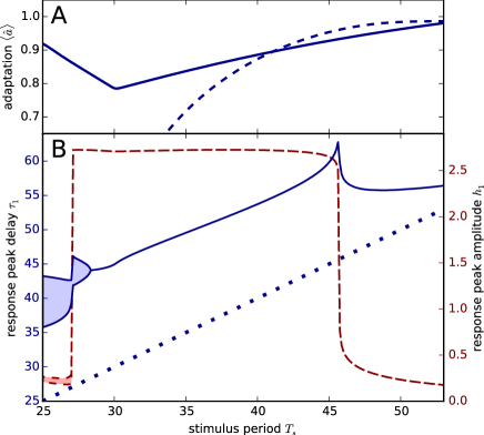
Figure 2: (Color online) A. The mean value of the adaptive variable $\left\langle\hat{a}\right\rangle$ under periodic stimulus as a function of the stimulus period (solid line) compared with the value of $a$ in a non-adaptive FHN oscillator that satisfies $T_{\text{fn}}\left(a\right)=T_{s}$ (dashed line). B. Delay time of first omitted stimulus response peak $\tau_{1}$ (solid line, left scale) as a function of stimulus period compared to $\tau_{1}=T_{s}$ (dotted line). The dashed curve (right scale) shows the amplitude of the response peak. The curves split into shaded area when the driven system does not settle into a simple limit cycle. The parameters for the adaptive dynamics are $a_{0}=1.4$ and $p=0.4$.

Simulations similar to that shown in Fig. 1 have also been performed for various stimulation periods. As expected, the $\left\langle\hat{a}\right\rangle$ in the synchronized state is a function of stimulation period (see Fig. 2A). That is, the information of the stimulation period can be stored in $\left\langle\hat{a}\right\rangle$. With the stored synchronized state $a=\left\langle\hat{a}\right\rangle$, the anticipative dynamics or OSR can be seen when $a$ relaxes back to $a_{0}$ after the external stimulation has been removed. In a sense, the OSR or anticipative dynamics is the byproduct of the adaptation.

Ideally, one expect the sustained oscillation periods will match the period of the stimulus input $T_{s}$, the position $a\approx\left\langle\hat{a}\right\rangle$ of the driven limit cycle should satisfy

$$T_{\text{fn}}\left(\left\langle\hat{a}\right\rangle\right)\approx T_{s}.$$ (6)

where $T_{\text{fn}}\left(a\right)$ denotes the oscillation periods in the original FHN system with a static $a$. The inverse $T_{\text{fn}}^{-1}\left(T_{s}\right)$ is shown as the dashed line in Fig. 2A. The value of $\left\langle\hat{a}\right\rangle$, which is a function of the stimulus period, is plotted as solid line in Fig. 2. The condition (6) implies two of the curves should coincide with each other. However, we see significant deviation even in the region where the first OSR retains the stimulus period well (see Fig. 2B). This suggests that other variables additional to $a$, such as the phase information in cycle of $v$-$w$ oscillations, are also contributing to the encoding of the periodicity information. Since we are interested in the general phenomena of a functioning anticipation, we will focus on the role of a single adaptive parameter for the current study. Additionally, one can constrain the dynamics of $a$ so that condition (6) is satisfied, or so that one would have $\bar{g}=T_{\text{fn}}^{-1}\left(T_{s}\right)$ for the average of (4). This likely involves optimizations specific to the systems of interests and can be a subject of future studies.

Following Schwartz et al. (2007), the effectiveness of rhythmic memory can be assessed by the timing of the first OSR peak right after the stop of the periodic stimulus. Typically, the retention of the information about stimulus period requires a one-to-one mapping of the period to the latency. As shown in Fig. 2B, the linear relation of the first OSR time with the stimulus period at $p=0.4$ and $a_{0}=1.4$ shows a good retention of the stimulus-period information: Comparing with the stimulus period, the latency $\tau_{1}$ has a constant delay of 15 units for the range of stimulus period from 28 to 45. Such a delay depends on the details of the model and can be interpreted as the time taken by the system to respond to the missing stimulus. Well-timed OSR similar to Fig. 2B can also be obtained for, say, a different value of $p$ or $\tau_{a}$ when the value of $a_{0}$ is properly chosen Note (1). As expected from the finite oscillation range of our reduced FitzHugh-Nagumo model, the amplitude of OSR peak drops significantly outside this range. For a fast stimulus (small $T_{s}$ as indicated by the shaded area in Fig. 2B), the system may not be able to settle into a simple limit cycle with the same small period, leading to a more complex behavior similar to the observation in Cortes et al. (2013). While, for a slow stimulus, the system will return to the quiescent fixed point before producing an OSR.

In our conceptual model, it should be clear that all we need to implement anticipative dynamics in an excitable system is an adaptive excitability. Interestingly, such a mechanism has already been used in the modeling of working memory (WM). Mongillo et al. Mongillo et al. (2008) consider WM as the result of the interactions between synaptic facilitation and depression. As illustrated in Fig. 3, anticipative dynamics can also be observed in such WM model . In a mean-field approximation Wilson and Cowan (1972), the neocortical network in Mongillo et al. (2008) is described by the firing rate $E$ of the neural tissue, the available neurotransmitter fraction $x$, and the probability of synaptic release $u$ (see supplementary material of Mongillo et al. (2008)). The parameter $u$ there plays a similar role as $a$ in our FHN model, namely, the value of $u$ determines whether the stationary state of the system is at a stable fixed point or on a limit cycles. Furthermore, the adaptation dynamic of $u$ comes from synaptic facilitation Tsodyks et al. (1998); Mongillo et al. (2008) and relates to the calcium concentration of the presynaptic cell. One interpretation of such relation is that the perception of time is being stored in the calcium concentration in these cells.

Figure 3: (Color online) Anticipative behavior of mean-field dynamics for a network model of working memory Mongillo et al. (2008) (see Note (1)). The trajectory and attractor manifold are similar to that described in Fig. 1B. The inset shows time course of the network firing rate $E$ driven by a square-wave stimulus (shaded) and its residual oscillations after the stimulus stops.

In a broader view of these systems, the transient, anticipative oscillations following the end of the periodic stimulus are similar to the burster dynamics found in neurosciences Izhikevich (2006) where a slow variable drive the system in and out of an oscillatory region of the state space. Since the adaptive dynamics is much slower than the oscillation, the trajectories of these systems mostly follow their attractor manifolds as shown in Figs. 1B and 3. The deviations from the manifolds will diminish with further increase of the slowness. In this limit, the nature of the bifurcations is likely important in determining how the system will return to the quiescent state. On the other hand, the retention of the periodicity information in the stimulus is controlled by the adaptive dynamics which sets the position of the driven limit cycle of the system. This information is released after the end of the stimulus and its manifestation is determined by the position of this endpoint in the state space relative to the attractor manifold. Our finding that the periodicity information is retained in the calcium level in the WM of Mongillo et al. (2008) is consistent with a recent report that time perception disorders are related to WM impairment Roy et al. (2012). In fact, experiments Lau and Bi (2005) have shown that network reverberations which is believed to be related to WM are controlled by residual calcium level in the synapses.

We restrict the current model to the simplest dynamics of adaptation under a periodic stimulus. We show the information of stimulus period can be well retained with anticipative responses in accord with the input. Such simplicity is not without limitations. For example, with a single adaptive parameter, the return to the quiescent state will be crossing the same region of the state space, which implies a necessary degradation of the periodicity information before the OSR subsides. To have an anticipative response that is transient and immune to degradation, a more complex model, i.e., with more variables or involving a bifurcation of higher codimensions Izhikevich (2000), is likely required but beyond our current discussion. On the other hand, experimental observations of such degradation in the periods of OSR will be strongly indicative of a similar simplistic mechanism at work.

The use of an adaptive system to fill a biological function has the benefit of being continuously tunable and allows easier optimization on a locally smooth landscape. Such mechanism has a lower circuitry design cost and is better suited for recurrent environmental conditions with varying time periods. As we have shown in this paper, the perception of time of such systems resides in the slowest dynamics involved, that is, the adaptive parameter $a$ in our case, or the synaptic calcium level for a neocortical network.

This work has been supported by the Ministry of Science and Technology, ROC under grand no. 102-2112-M-001 -009 -MY3, and National Center for Theoretical Sciences, NCTS-SOFT/1502.

References

- Pikovsky and Kurths (2003) A. Pikovsky and J. Kurths, Synchronization: A Universal Concept in Nonlinear Sciences (Cambridge University Press, 2003) 00004.
- Gros (2011) C. Gros, Complex and Adaptive Dynamical Systems, 2nd ed. (Springer, Berlin, Heidelberg, 2011) 00000.
- Zlotnik et al. (2013) A. Zlotnik, Y. Chen, I. Z. Kiss, H.-A. Tanaka, and J.-S. Li, Physical Review Letters 111, 024102 (2013), 00013.
- Winfree (2001) A. T. Winfree, The Geometry of Biological Time (Springer Science & Business Media, 2001) 00020.
- Schwartz et al. (2007) G. Schwartz, R. Harris, D. Shrom, and M. J. Berry, Nature Neuroscience 10, 552 (2007), 00032.
- Saigusa et al. (2008) T. Saigusa, A. Tero, T. Nakagaki, and Y. Kuramoto, Physical Review Letters 100, 018101 (2008), 00147.
- Sumbre et al. (2008) G. Sumbre, A. Muto, H. Baier, and M.-M. Poo, Nature 456, 102 (2008).
- Bueti et al. (2010) D. Bueti, B. Bahrami, V. Walsh, and G. Rees, Journal of Neuroscience 30, 4343 (2010), 00040.
- Mi et al. (2013) Y. Mi, X. Liao, X. Huang, L. Zhang, W. Gu, G. Hu, and S. Wu, Proceedings of the National Academy of Sciences 110, E4931 (2013).
- Mongillo et al. (2008) G. Mongillo, O. Barak, and M. Tsodyks, Science 319, 1543 (2008).
- FitzHugh (1961) R. FitzHugh, Biophysical Journal 1, 445 (1961).
- Note (1) Please see Supplementary Materials at [PRE website] for derivation of relation (5) and the parameter dependency of OSR timing.
- Cortes et al. (2013) J. M. Cortes, M. Desroches, S. Rodrigues, R. Veltz, M. A. Munoz, and T. J. Sejnowski, Proceedings of the National Academy of Sciences 110, 16610 (2013), 00004.
- Note (2) To have a quiescent state in the absence of external input, we use a slightly modified gain function from the Supporting Online Material of Mongillo et al. (2008).
- Wilson and Cowan (1972) H. R. Wilson and J. D. Cowan, Biophysical Journal 12, 1 (1972).
- Tsodyks et al. (1998) M. Tsodyks, K. Pawelzik, and H. Markram, Neural Computation 10, 821 (1998).
- Izhikevich (2006) E. M. Izhikevich, Dynamical Systems in Neuroscience: The Geometry of Excitability and Bursting, 1st ed. (The MIT Press, 2006).
- Roy et al. (2012) M. Roy, S. Grondin, and M.-A. Roy, Psychiatry Research 200, 159 (2012), 00007.
- Lau and Bi (2005) P.-M. Lau and G.-Q. Bi, Proceedings of the National Academy of Sciences 102, 10333 (2005).
- Izhikevich (2000) E. M. Izhikevich, International Journal of Bifurcation and Chaos 10, 1171 (2000).