Correct quantum chemistry in a minimal basis from effective Hamiltonians

Abstract

We describe how to create ab-initio effective Hamiltonians that qualitatively describe correct chemistry even when used with a minimal basis. The Hamiltonians are obtained by folding correlation down from a large parent basis into a small, or minimal, target basis, using the machinery of canonical transformations. We demonstrate the quality of these effective Hamiltonians to correctly capture a wide range of excited states in water, nitrogen, and ethylene, and to describe ground and excited state bond-breaking in nitrogen and the chromium dimer, all in small or minimal basis sets.

1 Introduction

The rapid evolution of quantum chemistry over the last decades means that in many molecules ^{1, 2, 3, 4} and even in some condensed phase systems ⁵, the combination of many-electron correlation methods with large basis sets provides predictions to beyond chemical accuracy of 1 kJ/mol. Despite these numerical advances, qualitative chemical and physical reasoning necessarily remains rooted in simple concepts.

One way to connect quantitative calculations to qualitative understanding is to construct an effective Hamiltonian to describe the correct correlated behaviour in terms of only the minimal chemical degrees of freedom, i.e. a minimal basis. Semi-empirical methods define such Hamiltonians by fitting to precomputed observables, but relying on empirical parametrization removes many advantages of predictive computation. A more satisfying route to effective minimal basis Hamiltonians is via rigorous ab-initio many-body theory. In this work, we will construct minimal basis effective Hamiltonians by rigorous many-body canonical transformations. While in principle an exact procedure, in practice approximations are necessary. We will thus be primarily concerned with addressing two questions of approximation. First, how do we define a simple, cheap, and stable, approximate canonical transformation to obtain the effective minimal basis Hamiltonian? And second, how well do such minimal basis Hamiltonians capture non-trivial chemistry, at least at a qualitative level?

We must use an effective as opposed to a bare Hamiltonian in a minimal basis because it is well established that quantum chemistry with the bare minimal basis Hamiltonian is exceedingly poor. This is because the electrons in filled orbitals cannot avoid each other, and the Coulomb interaction is felt too strongly. Modifying the Coulomb interaction to take into account excursions of electrons into orbitals external to the minimal basis is referred to as folding in the (effects of the) external orbitals. Alternatively, since the effective Coulomb interaction is decreased in magnitude, this process is often referred to as screening.

The effective Hamiltonian of interest depends in part on the choice of many-body formalism. For example, in Green’s function approaches, we can define an effective two-particle (four-point) interaction operator $\Gamma(1234)$ (where the labels $1,2,3,4$ include both time and orbital indices) that yields the appropriate two-particle (four-point) Green’s function $K(1234)$ in the minimal basis, using a Dyson-like equation ⁶

$$K=(GG)+(GG)\Gamma(GG)$$ (1)

where $G$ is the single-particle Green’s function. The interaction operator $\Gamma$ depends on time. When limited to the particle-hole channel, it is called the screened interaction, and is commonly computed within the random-phase approximation ^{7, 8}.

Here, however, we are concerned with the effective Hamiltonian $\bar{H}$ to be used in the many-body Schrödinger equation in the minimal basis,

$$\bar{H}|\Phi_{i}\rangle=E_{i}|\Phi_{i}\rangle$$ (2)

The state $|\Phi_{i}\rangle$ exists only in the Hilbert space of the minimal basis, but is related to the exact eigenstate $|\Psi_{i}\rangle$ in the full space by a many-body canonical transformation $|\Psi_{i}\rangle=U|\Phi_{i}\rangle$, thus $\bar{H}=U^{\dagger}HU$. Unlike the interaction operator $\Gamma$, the effective Hamiltonian $\bar{H}$ is time-independent, but in general contains three-body and higher body terms. The Hilbert space that $|\Phi_{i}\rangle$ lives in can be thought of as spanned by a basis of quasi-particles associated with second-quantized operators $\bar{a}^{({\dagger})}=U^{\dagger}a^{({\dagger})}U$.

The basic formalism of (canonically transformed) effective Hamiltonians is very old and well-known. There are two families of approximation methods. The first focuses on the effective Hamiltonian itself and dates all the way back to Van Vleck ⁹ and other early workers such as Brandow ¹⁰, Westhaus ¹¹, Freed ^{12, 13}, and others ¹⁴. Also in the first family are the renormalization group approaches to $\bar{H}$, based on successive iterative approximations, as developed by Wegner ¹⁵, Glazek and Wilson ¹⁶, and White ¹⁷. The second family of methods focuses more on the eigenstates $\ket{\Psi_{i}}$ and their associated wave operator. This includes the many variants of coupled cluster theory ¹⁸, and especially the equation-of-motion ¹⁹ and multireference extensions ²⁰. There is much overlap between the families and there are methods which belong to both (such as the earlier canonical transformation work of Yanai, Neuscamman, and Chan ^{21, 22, 23, 24}, the anti-Hermitian contracted Schrödinger equation of Mazziotti ^{25, 26}, and the recent similarity renormalization group work of Evangelista ²⁷). However, a defining difference is that in the presence of degeneracies and strong correlations, the first family usually adopts a “perturb and diagonalize” strategy, while the second performs “diagonalize and perturb”. This difference is one of philosophy but can lead to different choices in approximations.

We are concerned here with techniques in the first family to construct effective minimal basis Hamiltonians. The earlier works by Freed, and by White, and especially the recent work by Yanai and Shiozaki ²⁸ are, in our view, conceptually the most closely related. We will explore the approach of Yanai and Shiozaki in parallel to the new approaches in this work. In addition, the numerical approximations we use build on the earlier work on approximate canonical transformations by Yanai, Neuscamman, and Chan.

In Section 2 we begin by precisely defining the effective Hamiltonian in a minimal basis. We then outline the earlier approximate canonical transformation formalism of Yanai, Neuscamman, and Chan, and next the detailed steps and approximations to construct the effective minimal basis Hamiltonians in this work. We proceed to assess the performance of our effective Hamiltonians for a variety of chemical phenomena, including electronic excited states and potential energy surfaces. We finish with a discussion of some future directions of this approach.

2 Theory

2.1 The effective Hamiltonian

We begin with some notation. The effective Hamiltonian folds the effects of electron correlation from an initial large (possibly infinite) “parent” basis down to a smaller “target” basis. We label orbitals in the parent basis (assumed orthogonalized) by indices $\{\kappa,\lambda,\mu,\nu\}$. Thus the parent basis Hamiltonian is written as

$${H}=\sum_{\mu\nu}h_{\mu\nu}{E}_{\mu\nu}+\frac{1}{4}\sum_{\mu\nu\kappa\lambda}V_{\mu\nu\kappa\lambda}{E}_{\mu\nu\lambda\kappa}$$ (3)

where we use the spin-summed excitation operators ${E}_{\mu\nu}=\sum_{\sigma\in\{\alpha,\beta\}}a^{\dagger}_{\mu\sigma}a_{\nu\sigma}$, and $V_{\mu\nu\kappa\lambda}$ represents the anti-symmetrized two-electron integral operator.

We label the target basis (assumed orthogonalized) by $\{p,q,r,s\}$. In this work, we take the target basis to be spanned by a set of minimal Gaussian basis functions, although in principle any small basis can be used. The (orthogonal) functions that are in the parent basis but which live outside of the target basis, define the external space; we will label these by $\{x,y\}$. When the parent basis is formally infinite (as in R12/F12 theory), the external space is represented, as necessary, by its complementary auxiliary basis ²⁹ (discussed in detail in Section 2.4). Note that for two arbitrary finite parent and target Gaussian bases, the target basis is not usually a subspace of the larger parent basis. In that case, we consider the parent basis to be the union of the target basis and the original parent basis. For example, if using an ANO-RCC-MIN target basis ³⁰ and an aug-cc-pVQZ ³¹ parent basis, we take the parent basis in numerical calculations to be ANO-RCC-MIN+aug-cc-PVQZ. The dimension of the external space is then the same as that of the original parent basis.

The exact effective Hamiltonian in the target basis is

$${\bar{H}}=\bar{h}_{pq}{E}_{pq}+\frac{1}{4}\bar{V}_{pqrs}{E}_{pqrs}+\frac{1}{36}\bar{W}_{pqrstu}{E}_{pqrstu}+\ldots$$ (4)

where $\ldots$ indicates additional higher-body interactions. ${\bar{H}}$ is related to $H$ by the canonical transformation operator $e^{A}$, using the Baker-Campbell-Hausdorff (BCH) expansion,

$${\bar{H}} =e^{A^{\dagger}}He^{A}$$

$$={H}+\left[{H},{A}\right]+\frac{1}{2}\left[[{H},{A}],{A}\right]+\ldots$$ (5)

where $A$ is the antihermitian excitation and de-excitation operator between the target and external space. $A$ can be written in terms of 1-body, 2-body, and higher components,

$${A} ={A}_{1}+{A}_{2}+\ldots$$

$$=\sum_{px}t_{px}\left({E}_{xp}-{E}_{px}\right)+\frac{1}{4}\sum_{pqxy}t_{pqxy}\left({E}_{xypq}-{E}_{pqxy}\right)+\ldots$$ (6)

The amplitudes of $A$: $t_{px}$, $t_{pqxy}$, etc., are chosen to make all matrix elements between the target and external spaces vanish. This leads to equations of the form of generalized Brillouin conditions ^{32, 21},

$$\langle\Phi|[{\bar{H}},\left({E}_{px}-{E}_{xp}\right)]|\Phi\rangle =0,$$

$$\langle\Phi|[{\bar{H}},\left({E}_{pqxy}-{E}_{xypq}\right)]|\Phi\rangle =0,\ldots$$ (7)

where $\ket{\Phi}$ is any state in the target space. The complete Brillouin conditions define ${\bar{H}}$ uniquely, up to decoupled rotations within the target and external spaces separately.

In the above equations we immediately observe the need for approximation. This arises in (i) truncating $A$ in Eq. (6), (ii) handling the BCH expansion of ${\bar{H}}$ and the many-body interactions in Eqs. (4), (5), and (iii) solving the amplitude equations, Eq. (7). We now discuss approximations in each of these areas.

2.2 Approximate canonical transformations

In defining approximate canonical transformations we are motivated by the prior experience of Yanai, Neuscamman, and Chan ^{21, 22, 33, 24} and Yanai and Shiozaki²⁸, and by the accuracy requirements in this work. Our goal here is qualitative accuracy for a broad range of phenomena, rather than highly quantitative (e.g. 1 kcal/mol) chemical accuracy for a particular single target state at a given geometry.

For (i) and (ii), we re-use the main ideas in Yanai, Neuscamman, and Chan, namely we truncate amplitudes at the two-body level ($A=A_{1}+A_{2}$) and limit the effective Hamiltonian to two-body interactions by approximating higher-body terms. For qualitative accuracy, it is reasonable to truncate the BCH expansion through second-order perturbation theory as in the work of Yanai and Shiozaki. This gives $\bar{H}$ as

$${\bar{H}}\approx H+\left[{H},{A}\right]+\frac{1}{2}\left[[{F},{A}],{A}\right]$$ (8)

where $F$ is a Fock operator (defined more precisely below). If $F$ is defined using the Hartree-Fock density matrix, the expectation value of ${\bar{H}}$ with the Hartree-Fock determinant $\bra{\Phi_{D}}\bar{H}\ket{\Phi_{D}}$ is the Hylleraas second-order energy functional.

Note that although accurate only through second-order, the effective Hamiltonian in Eq. (8) already involves three-body interactions, generated by the first and second commutators. However, approximating $\bar{H}$ by a two-body Hamiltonian is well supported by the success of semi-empirical and model Hamiltonians, which universally assume only two-body interactions. Decomposing three- and higher-body interactions into effective two-body interactions was already considered by Iwata and Freed in the effective valence Hamiltonian theory ¹³. In the canonical transformation theory of Yanai and Chan, this decomposition was systematized using the generalized normal ordering of Mukherjee and Kutzelnigg ³⁴ (an extension of the density cumulant expansion to operators) ^{35, 36, 37}. This re-expresses the 3-body operators generated above, $E^{pqr}_{stu}$, by

$$a^{pqr}_{stu}\approx 9(\gamma^{p}_{s}\wedge a^{qr}_{tu})-36(\gamma^{p}_{s}\wedge\gamma^{q}_{t}\wedge\gamma^{r}_{u})+9(\gamma^{pq}_{st}\wedge a^{r}_{u})+24(\gamma^{p}_{s}\wedge\gamma^{q}_{t}\gamma^{r}_{u})-9(\gamma^{pq}_{st}\wedge\gamma^{r}_{u})$$ (9)

where we drop explicit 3-body fluctuation operators and 3-body density cumulants. (The above term $a^{pqr}_{stu}$ is expressed in terms of spin-orbitals. The correct spin-summed expression is given in Ref. ³⁸, but we use the spin-orbital decomposition in our implementation). Since both the cumulants and the expectation value of the 3-body fluctuation operators vanish for a determinant state, truncating the 3-body terms in Eq. (9) preserves the expectation value of ${\bar{H}}$ with any determinant, and thus the value of the standard Hylleraas functional. Denoting the truncated normal ordering approximation in Eq. (9) by the subscript $(1,2)$, we obtain the approximate two-body $\bar{H}_{(1,2)}$ as

$${\bar{H}}_{(1,2)}={H}+\left[{H},{A}\right]_{(1,2)}+\frac{1}{2}\left[[{F},{A}],{A}\right]_{(1,2)}$$ (10)

When not ambiguous, we drop the subscript $(1,2)$ in the labelling of ${\bar{H}}_{(1,2)}$, understanding that it is defined as above.

Both the Fock matrix $F$ and the normal ordering approximation in Eq. (9) require density matrices, thus introducing state-specific information. To minimize the amount of initial state-specific computation with the bare Hamiltonian (in keeping with the perturb and diagonalize philosophy) we use only density matrices from the Hartree-Fock ground-state in the target basis unless otherwise specified.

2.3 Approximate amplitudes

We next discuss how to determine the amplitudes. In the original canonical transformation work of Yanai and Chan, the amplitude equations are solved with respect to an initial (multireference) state $|\Psi_{0}\rangle$, typically a ground-state complete active space wavefunction, using the normal-ordered approximate $\bar{H}$ and the Brillouin conditions in Eq. (7) with $|\Phi\rangle=|\Psi_{0}\rangle$. This provides a route to add dynamic correlation to the strong correlations presumed captured by $\ket{\Psi_{0}}$. However, there are several reasons not to use this strategy here. First, solving the amplitude equations for a multireference $\ket{\Psi_{0}}$ is expensive - similar in scaling to, but several times the cost of, a coupled cluster singles doubles calculation. This is overkill for the qualitative accuracy we target. More importantly, there are fundamental numerical issues when solving the Brillouin conditions. The Jacobian of Eq. (7) has small eigenvalues, and without a cutoff of these eigenvalues hundreds of iterations of the equations may be required. These small Jacobian eigenvalues also appear in internally contracted multi-reference coupled cluster theory ^{39, 40, 41, 42} as well as in the anti-Hermitian contracted Schrödinger equation ^{25, 26} (mathematically equivalent to a Schrödinger picture formulation of the Brillouin conditions) leading to convergence difficulties in both these methods.

Further, at a fundamental level, the small Jacobian eigenvalues arise because the amplitude equations are solved for a single reference state $|\Psi_{0}\rangle$, which may have no weight in certain orbitals or electron configurations in the target space. Thus the amplitudes obtained are biased towards the reference state. This is an advantage for high accuracy for a given state (as in the original canonical transformation theory, or as in coupled cluster theory) but is a liability for a qualitative effective Hamiltonian intended to describe many states on an equal footing.

For both these reasons, here we construct approximate amplitudes in a manner that does not require the iterative solution of ill-conditioned and state-specific equations. We start with an effective Hamiltonian defined by the Hylleraas expression in Eq. (10), and use a Fock operator $F$ built from the Hartree-Fock density matrix in the small target basis. Re-expressing this in the parent basis, $F$ can be written in semi-canonical form, for computational efficiency, as

$$\mathbf{F}=\left[\begin{array}[]{cccc}F_{ij}\delta_{ij}&0&\ddots\\ 0&F_{ab}\delta_{ab}&\ddots\\ \ddots&\ddots&F_{xy}\delta_{xy}\\ \end{array}\right]$$ (11)

where $i,j$ and $a,b$ denote occupied and virtual molecular orbitals of the Fock operator in the target basis, respectively. The solution of the Brillouin condition with $\ket{\Phi}=\ket{\Phi_{D}}$ (where $\Phi_{D}$ is the target basis Hartree-Fock Slater determinant) is the Moller-Plesset first-order wavefunction, with amplitudes

$$t_{ix} =\frac{F_{ix}}{\epsilon_{i}-\epsilon_{x}}$$

$$t_{ijxy} =\frac{V_{ijxy}}{\epsilon_{i}+\epsilon_{j}-\epsilon_{x}-\epsilon_{y}}$$ (12)

where $\epsilon_{i}=F_{ii}$, $\epsilon_{x}=F_{xx}$, respectively. We can now use these amplitudes to construct $\bar{H}$. The singles and doubles amplitudes respectively add the Hartree-Fock basis set correction from the external space, and the correlated MP2 contribution from the external space, to the zeroth order Hartree-Fock energy of $\bar{H}$.

Note, however, that the amplitudes in Eq. (12) are defined only between orbitals occupied in $\ket{\Phi_{D}}$ $i,j$, and the external orbitals $x,y$. To decouple other low-lying states in the target basis from the external space, we consider using other (non-ground-state) determinants $\ket{\Phi_{D}^{\prime}}$ to define the amplitudes in Eq. (12), which occupy “active virtual” orbitals $a,b,c$ (orbitals not occupied in the lowest determinant). This defines additional amplitudes involving the active virtuals, such as

$$t_{ax} =\frac{F_{ax}}{\epsilon_{a}-\epsilon_{x}}$$

$$t_{abxy} =\frac{V_{abxy}}{\epsilon_{a}+\epsilon_{b}-\epsilon_{x}-\epsilon_{y}}$$ (13)

and similar amplitudes with mixed (active and occupied) indices, such as $t_{ia}^{xy}$. Such amplitudes involving “active virtuals” are omitted in the definition of the effective Hamiltonian in equation-of-motion coupled cluster theory, because they annihilate the lowest Hartree-Fock ground-state $\ket{\Phi_{D}}$ and do not change the ground-state energy. However, they are necessary to remove the bias towards the ground-state in the resulting effective Hamiltonian. Unfortunately, if we use the additional amplitudes as naively written in Eq. (13), we obtain very poor results. This is because the virtual eigenvalues $\epsilon_{a}$, $\epsilon_{b}$ appearing in Eq. (13) are determined for the ground-state density matrix and Fock operator, rather than for the Fock operator corresponding to the excited state determinant $\ket{\Phi_{D}^{\prime}}$. As the eigenvalue difference between the active virtual orbitals and external orbitals often vanishes, Eq. (13) can even yield divergent amplitudes.

Physically, the energy of an electron in one of the active virtual orbitals $\phi_{a}$ is not well approximated by $\epsilon_{a}$, but is rather much closer to the HOMO energy level. This is because in Hartree-Fock theory the virtual energy levels are optimized in the field of $N$ rather than $N-1$ electrons. The appropriate orbital relaxation effect would be properly included if we retained three-body operators in the effective Hamiltonian (similar to treating triples excitations in coupled cluster theory) but are not properly captured in the $(1,2)$ approximation. To partially take into account this 3-body effect we now introduce a simple approximation. In the definition of amplitudes involving an active virtual orbital, we replace the corresponding virtual Fock energy $\epsilon_{a}$ by a single modified orbital energy, $\bar{\epsilon}_{a}$. In the simplest case, we replace $\bar{\epsilon}_{a}$ by the HOMO energy, but we can also view $\bar{\epsilon}_{a}$ as an adjustable parameter. (This modification of the active virtual denominators can also be justified from the viewpoint of degenerate perturbation theory, as argued by Iwata and Freed, who placed all occupied and active (valence) orbitals at the same average energy thus creating a truly degenerate zeroth order Hamiltonian ¹³). Thus,

$$t_{ax} =\frac{F_{ax}}{\epsilon_{x}-\bar{\epsilon}_{a}}$$

$$t_{ajxy} =\frac{V_{ajxy}}{\epsilon_{x}+\epsilon_{y}-\bar{\epsilon}_{a}-\epsilon_{j}}$$

$$t_{abxy} =\frac{V_{abxy}}{\epsilon_{x}+\epsilon_{y}-2\bar{\epsilon}_{a}}$$ (14)

With this regularization, we define $A$ to include all amplitudes involving the additional active virtual labels, except for active-active to active-external ($abcx$). Including the latter class of amplitudes tends to lead to significantly worse results, presumably because it requires a more rigorous treatment of the higher body effects than this simple effective denominator.

2.4 Comparison to the approach of Yanai and Shiozaki

In their work on canonical transcorrelated Hamiltonians, Yanai and Shiozaki used a simple definition of the amplitudes that also does not require the solution of amplitude equations, and which is appropriate when both the target and parent basis are large. Following Ten-no ⁴³, the first-order MP2 amplitudes in an infinite external basis are fixed by the cusp condition. Using an F12 factor $f=\exp(-\gamma r_{12})$ to represent the beyond linear terms in the $r_{12}$ dependence, one obtains MP2 amplitudes given by

$$t_{ij\alpha\beta}(F12)=\frac{1}{8}\langle\alpha\beta|{Q}_{12}{F}_{12}|ij\rangle+\frac{3}{8}\langle\alpha\beta|{Q}_{12}{F}_{12}|ji\rangle$$ (15)

where $\alpha,\beta$ label the formal infinite external parent basis, and $Q_{12}$ is the strong orthogonality projector ²⁸.

In this work, we replace the formal infinite basis by the large parent basis and view the formula (15) as a way to provide the corresponding amplitudes $t_{ix},t_{ax},t_{ijxy}$ etc. We can include orbital relaxation effects by defining the singles as in Eq. (12). $Q_{12}$ ensures that the F12 excitations are orthogonal to those in the target basis since

$$Q_{12}=(1-{p(1)})(1-{p(2)})-x(1)x(2)$$ (16)

and $p(1)$ denotes a (one-particle) projector onto the orbitals (occupied and active virtual) in the target space, and $x(1)$, to the external orbitals.

Using these F12-derived amplitudes, we then construct ${\bar{H}}$ directly using the BCH expansion in Eq. (8). Alternatively, Yanai and Shiozaki used approximation “C” of Kedžuch et al. ⁴⁴ to compute the double commutator $[[F,A],A]$: we denote the corresponding approximation, F12(C). The effective Hamiltonians computed in either approach are identical in the limit of a large parent basis, but for rapid convergence, one should choose the parent basis to be an auxiliary basis set specifically constructed for use in F12 theories.

Note that Eq. (15) defines not only the standard occupied to external amplitudes $t_{ij}^{xy}$, but also active virtual to external excitations $t_{ab}^{xy}$ as well. Thus using the complete set of F12 amplitudes (as in the earlier canonical transcorrelated Hamiltonian of Yanai and Shiozaki) also dresses the Hamiltonian for excited states. (Note that, following Yanai and Shiozaki, we do not include active-active to active-external semi-internal excitations). However, the amplitudes target only the universal part of the short-range correlations, as defined by the Coulomb cusp, and thus retain no state-specific information. Such state information is only represented by amplitudes in the target space. For this reason, we expect effective Hamiltonians derived using the universal F12 amplitudes to be less accurate than those obtained using the orbital MP2 coefficients in section 2.3 when folding into small target bases, such as a minimal basis.

3 Results and discussion

3.1 Effective minimal basis Hamiltonian energies

As a first check of our effective Hamiltonian construction, we compute second order perturbation theory (MP2) ground-state energies in the parent basis, using the bare Hamiltonian $H$, and the corresponding MP2 ground-state energies in the target basis, using the effective Hamiltonian defined in Eq. (10). For comparison, we also compute the MP2 ground-state energies in the target basis with the bare Hamiltonian, to show the effects of folding. To construct $\bar{H}$ we use both explicit orbital amplitudes (Sec. 2.3) as well as F12 amplitudes (Sec. 2.4). We recall that despite the $(1,2)$ approximation in the commutator expansion for $\bar{H}$, the MP2 energies (using explicit orbital amplitudes) in the parent and target basis should match exactly, up to orbital relaxation effects. The orbital relaxation effects are not captured completely simply because they are treated to infinite order in the Hartree-Fock calculation in the parent basis, but only to second order in our effective Hamiltonian.

Tables 1, 2 give the errors in the effective Hamiltonian MP2 energies relative to the parent basis for the water and nitrogen molecules. We use the single-$\zeta$ contraction of Roos’ ANO family of bases sets, labeled ANO-RCC-MIN, and Dunning’s family of cc-pVXZ (X $=$ D, T), labeled DZ and TZ target bases, and an aQZ parent basis (aXZ is Dunning’s aug-cc-pVXZ basis ⁴⁵). The quoted reference MP2 aQZ energy does not include the additional basis functions from the target basis, but this has a negligible effect relative to the errors that we are discussing; for example, the MP2 water energy using the aQZ basis is -76.38278 $E_{h}$, while using the union of the MIN and aQZ basis, it is -76.38405 $E_{h}$.

For $\bar{H}$ constructed from orbital amplitudes, the error in the effective ground-state energy, due to incomplete orbital relaxation, is small: [24] m$E_{h}$ and [37] m$E_{h}$ for water and nitrogen respectively, even in the smallest ANO-RCC-MIN target basis. This compares quite favourably with the error in the bare Hamiltonian ANO-RCC-MIN MP2 energy: 412 m$E_{h}$ and 529 m$E_{h}$ for water and nitrogen respectively. The error from incomplete orbital relaxation decreases as the target basis size increases.

Table 1: Difference between the MP2 ground-state energy in various target bases (ANO-RCC-MIN, DZ, TZ), and the MP2 aQZ (parent basis) ground-state energy, for the water molecule at the equilibrium geometry $R={1.80847~{}\text{\AA}},\theta={104.5^{\circ}}$. The $H$ column denotes the (standard) MP2 calculation with the normal bare Hamiltonian. The other columns refer to the calculations using the effective Hamiltonian. Orb. denotes $\bar{H}$ using orbital amplitudes, F12 denotes F12 amplitudes, F12(C) denotes using approximation “C” in the double commutator, and F12+$A_{1}$ denotes additional singles excitations. All energies in $E_{h}$. The MP2 aQZ energy is $-76.38278$ $E_{h}$. (The union of ANO-RCC-MIN and aQZ MP2 energy is $-76.38405$ $E_{h}$).

Target Basis	Error ($H$)	Error ($\bar{H}$)
		Orb.	F12	F12(C)	F12+$A_{1}$
ANO-RCC-MIN	0.4129	0.0247	0.2374	0.1933	0.1203
DZ	0.1520	0.0330	0.0760	0.0930	0.0412
TZ	0.0505	0.0095	0.0197	-0.0337	0.0119

Table 2: Difference between the MP2 ground-state energy in various target bases (ANO-RCC-MIN, DZ, TZ), and the MP2 aQZ (parent basis) ground-state energy, for the nitrogen molecule at the equilibrium geometry $R=1.09768\text{\AA}$. The $H$ column denotes the (standard) MP2 calculation with the normal bare Hamiltonian. The other columns refer to the calculations using the effective Hamiltonian. Orb. denotes $\bar{H}$ using orbital amplitudes, F12 denotes F12 amplitudes, F12(C) denotes using approximation “C” in the double commutator, and F12+$A_{1}$ denotes additional singles excitations. All energies in $E_{h}$. The MP2 aQZ energy is $-109.45124$ $E_{h}$. (The union of ANO-RCC-MIN and aQZ MP2 energy is -109.45259 $E_{h}$).

Target Basis	Error ($H$)	Error ($\bar{H}$)
		Orb.	F12	F12(C)	F12+$A_{1}$
ANO-RCC-MIN	0.5291	0.0374	0.3396	0.2531	0.1249
DZ	0.1865	0.0324	0.0787	0.0157	0.0453
TZ	0.0683	0.0075	0.0184	-0.0364	0.0107

For $\bar{H}$ constructed from the F12 amplitudes, using an aQZ CABS basis, the errors are somewhat larger. (These errors are measured relative to the MP2 aQZ energy. We could measure the error relative to the MP2-F12 aQZ energy, but as the difference between the MP2 and MP2-F12 aQZ energies is small on the scale of errors we are discussing ($1.3$ m$E_{h}$ for the water molecule) this would not change the conclusions. A measure of the CABS basis completeness is given by the difference between the F12 and F12(C) columns.) We observe several important things. First, the difference between the F12 and F12+$A_{1}$ columns, shows that the CABS single particle amplitudes are very important, as they capture orbital relaxation. Second, the F12 amplitudes lead to a significantly less accurate $\bar{H}$ than the explicit MP2 orbital amplitudes. This is because the F12 amplitudes do not capture the non-universal part of the short-range correlation.

3.2 Excitation energies

The purpose of the effective Hamiltonian, is, of course, not simply to reproduce the ground-state calculation from which it is constructed, but to be able to use it in new calculations. We therefore now examine the accuracy of the effective Hamiltonians for the excitation energies of water, nitrogen, and ethylene. Density matrix renormalization group (DMRG) was used for the water and nitrogen effective Hamiltonian and parent bases excited state calculations. The DMRG calculations used up to $M$=4000 (with $S^{2}$ symmetry) for both molecules and all states, and are converged to microHartree level ($1s$ electrons in nitrogen were kept frozen for all calculations). Ethylene effective Hamiltonian and parent bases excitation energies were computed using the equation of motion coupled cluster with connected single and double excitations and a perturbative treatment of triples (EOM-CCSD(T)).

Tables 3 and 4 give the lowest few excitation energies for the water and nitrogen molecules using the aforementioned ANO-RCC-MIN target basis, and Dunning’s DZ parent basis. We first examine the water molecule. The excitation energies using the bare ANO-RCC-MIN Hamiltonian are very poor, with a maximum error of 5.40 eV. The effective Hamiltonian using all orbital amplitudes (shifting the active virtual energies to $\bar{\epsilon}_{a}=0.2$ $E_{h}$) yields a very significant improvement with a maximum error now of only 0.45 eV, quite surprising for a calculation in a minimal basis! For comparison, if we use F12 amplitudes the errors of the effective Hamiltonian are essentially unchanged with respect to the bare Hamiltonian $H$, with a maximum error of -5.43 eV. This shows that the F12 amplitudes do not properly capture differential correlation between the ground and excited state in this molecule. Some part of the differential correlation is recovered using the additional $A_{1}$ amplitudes (F12+$A_{1}$), reducing the maximum error to 0.91 eV, but this is still worse than the effective Hamiltonian using explicit orbital amplitudes.

An important column in the table is the one labelled “no act.”. These show results where “active” orbitals are omitted from the amplitudes in the $\bar{H}$ construction. This has no effect on the ground-state energies in the previous section, but as we argued will significantly affect the excitations. We see that this effective Hamiltonian - which is in essence the Hamiltonian used in equation-of-motion coupled cluster theories - yields even worse excitation energies than the bare Hamiltonian, since it overcorrelates the ground-state and leads to unbalanced treatment of excitations. In equation-of-motion coupled cluster, this imbalance is ameliorated by rediagonalizing in the full orbital space (including the external orbitals), not just a small “active” space as is implicitly done here by diagonalizing in the minimal basis.

Column “$[[H,A],A]$” shows the results of using the full Hamiltonian operator, rather than the Fock operator, in the double commutator contribution to $\bar{H}$ in Eq. (10). Interestingly we find that the results using the Fock operator are uniformly better than using the true $H$. We attribute this to some form of error cancellation.

Table 3: Errors of effective Hamiltonian excitation energies compared to parent basis excitation energies of water (computed using DMRG with parameters mentioned in the text). Target (small) basis is ANO-RCC-MIN and parent basis is cc-pVDZ. Units are in electron Volts. State notation X.Y.Z denotes Multiplicity.Irrep.State (with State being energy ordered).

	Ref.	Bare $H$	${\bar{H}}$
State	DZ	ANO-RCC-MIN	Orb.a	$[[H,A],A]$a	no act.	F12	F12(C)	F12+$A_{1}$
3.3.1	7.46	3.49	-0.36	1.34	6.48	3.93	3.88	-0.91
1.3.1	8.13	4.24	-0.09	1.36	7.23	4.64	4.47	-0.69
3.2.1	9.73	4.56	-0.08	1.93	7.20	4.85	4.82	-0.67
3.1.1	9.89	3.24	-0.38	6.86	6.31	3.48	3.40	-0.86
1.2.1	10.15	5.04	0.03	1.92	7.62	5.27	5.14	-0.55
1.1.2	10.80	4.43	-0.23	1.07	7.66	4.48	4.30	-0.44
3.4.1	11.90	3.59	-0.28	1.57	6.16	3.83	3.74	-0.85
1.4.1	12.86	5.40	0.45	2.14	8.21	5.43	5.21	0.11

• $\epsilon_{a}$ set to $-0.20$ a.u.

Table 4: Errors of effective Hamiltonian excitation energies compared to parent basis excitation energies of water (computed using DMRG with parameters mentioned in the text). Target (small) basis is ANO-RCC-MIN and parent basis is cc-pVDZ. Units are in electron Volts. State notation X.Y.Z denotes Multiplicity.Irrep.State (with State being energy ordered).

			${\bar{H}}$
State	DZ	ANO-RCC-MIN	Orb.a	$[[H,A],A]$a	no act.	F12	F12(C)	F12+$A_{1}$
3.6.1	7.83	0.57	0.28	0.64	1.90	0.77	0.67	0.33
3.3.1	8.12	-0.56	0.68	0.84	2.58	-0.47	-0.57	0.56
3.5.1	9.13	0.85	0.42	0.60	2.18	0.95	0.75	0.46
1.3.1	9.54	-0.66	0.77	0.93	2.72	-0.50	-0.79	0.50
3.5.2	9.93	0.71	0.34	0.48	2.24	0.76	0.52	0.29
1.5.1	10.26	1.10	0.54	0.58	2.47	1.12	0.84	0.57
1.6.1	10.65	1.05	0.51	0.47	2.46	1.04	0.69	0.47

• $\epsilon_{a}$ set to $-0.30$ a.u.

The excitation energies for nitrogen in Table 4 follow a similar trend to those seen for water. The main difference is that the excitation energies from the bare Hamiltonian in the target ANO-RCC-MIN basis are not too far from those in the parent DZ basis (maximum error of -1.1 eV). We thus expect folding to an effective minimal basis Hamiltonian to yield less of an improvement, and indeed that is the case. Using the effective Hamiltonian with orbital amplitudes, the maximum error is reduced to -0.77 eV. The relative performance of the F12 amplitudes and orbital amplitudes follow a similar trend to what is seen in the water molecule: the F12 amplitudes alone lead to little or no improvement in the excitation energies.

Figures 1,  2, 3 present correlation plots of the bare and effective Hamiltonian excitation energies, for the low-lying excitation energies of the water, nitrogen, and ethylene molecules. (These were generated as the 4 lowest energy states within each irrep, for each multiplicity). We show results for the bare Hamiltonian in DZ and TZ bases, and the effective Hamiltonian in a ANO-RCC-MIN basis. Statistical data for the excitation energies of water and nitrogen are also given in Tables 5, 6.

All plots clearly show the very substantial improvement brought about by using the effective Hamiltonian, rather than the bare Hamiltonian. The excitation energies (points) for the bare target basis Hamiltonian are quite far from the exact (parent basis) energies. In the case of water and ethylene they are too high, while for nitrogen they are scattered around the parent basis results. Folding yields effective Hamiltonians with excitation energies tightly clustered around the parent results.

The figures also show the influence of the choice of energies for the active virtuals. As we saw for the first few excited states above, using no active virtuals in the effective Hamiltonian construction leads to very poor excitation energies, worse than using the bare Hamiltonian alone. Using active virtuals and shifting them to the HOMO energy greatly improves the results, and choosing an optimal energy of the active virtuals improves them further. This is also seen through the statistical tables: for example, for water in the DZ basis, using the effective minimal basis Hamiltonian reduces the RMSD error from 6.72 eV (bare Hamiltonian) to 1.79 ($\bar{\epsilon}_{a}$ = HOMO energy) and 1.05 eV ($\bar{\epsilon}_{a}=-0.3$ eV). For nitrogen, as discussed earlier, the minimal basis excitation energies are reasonably accurate, and we observe a less dramatic reduction of the RMSD error, from 1.24 eV to 1.01 eV ($\bar{\epsilon}_{a}=-0.3$ eV).

In explicitly correlated theory, it is common to refer to the effect of including an explicit F12 correlation factor as increasing the “zeta” level of the calculation, for example, turning a DZ ground-state quality calculation into a QZ quality calculation. In a similar way, we ask, if we use a very large parent basis, how much does that increase the “$\zeta$” level of the effective Hamiltonian target basis calculation? In Fig. 1 we further compare the errors of excitations (measured from TZ basis excitations) with those from an effective ANO-RCC-MIN Hamiltonian derived from the TZ parent basis, and an explicit (bare Hamiltonian) DZ calculation. We find that the canonical transformation approximately achieves one additional $\zeta$ level of quality.

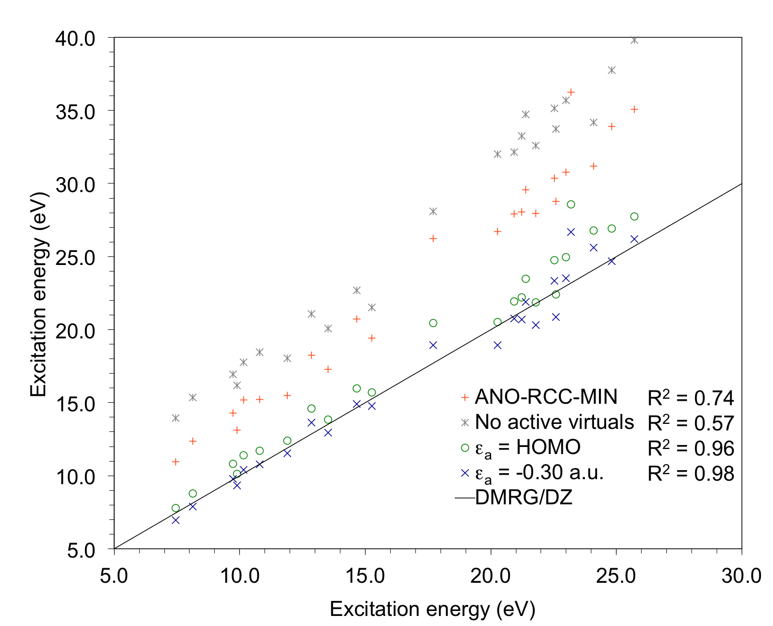
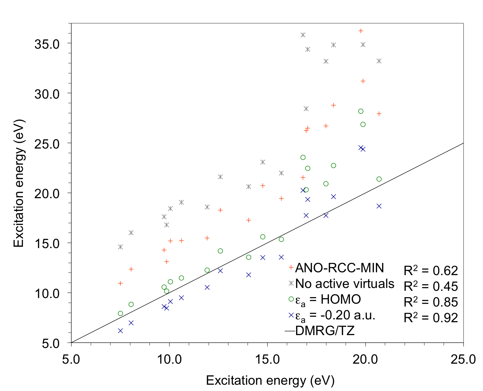
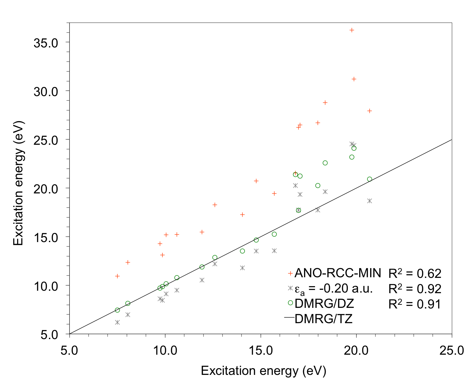
Figure 1: Correlation plots for excitation energies of the water molecule with the target ANO-RCC-MIN effective Hamiltonian, compared to the excitation energies in the parent basis (cc-pVDZ (left), cc-pVTZ (right)). The bottom chart compares the excitation energies of a target ANO-RCC-MIN effective Hamiltonian (parent cc-pVTZ basis) and excitation energies of a bare cc-pVDZ Hamiltonian with the parent cc-pVTZ excitation energies, to see the “$\zeta$” level of improvement due to canonical transformation. (Excitation energies computed using DMRG).

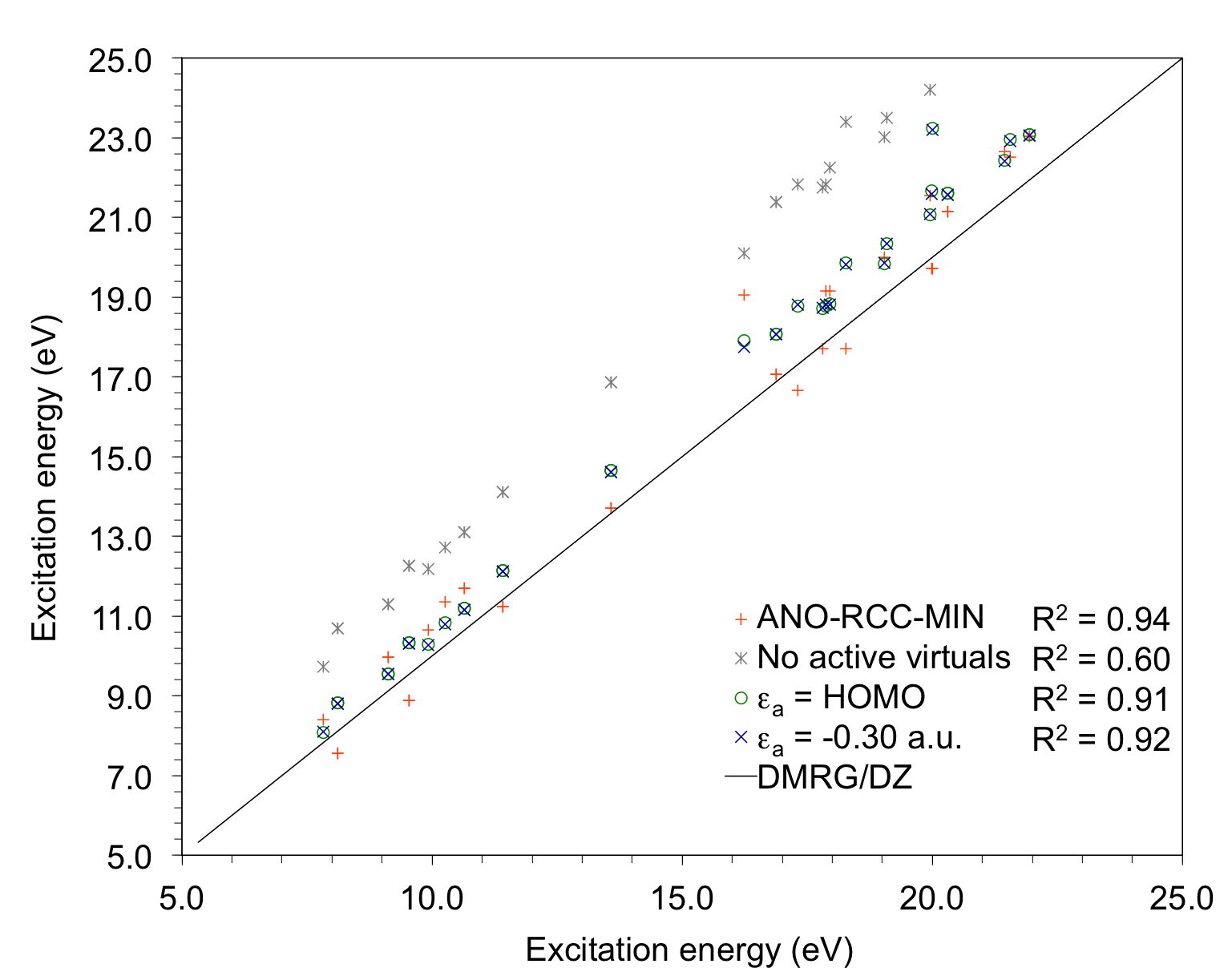
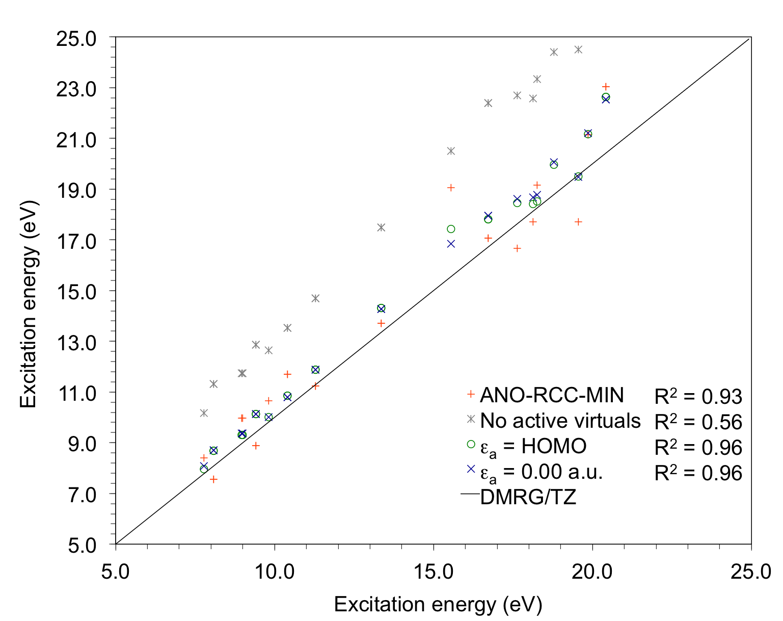
Figure 2: Correlation plots for excitation energies of the nitrogen molecule with the target ANO-RCC-MIN effective Hamiltonian, compared to the excitation energies in the parent basis (cc-pVDZ (left), cc-pVTZ (right)). (Excitation energies computed using DMRG).

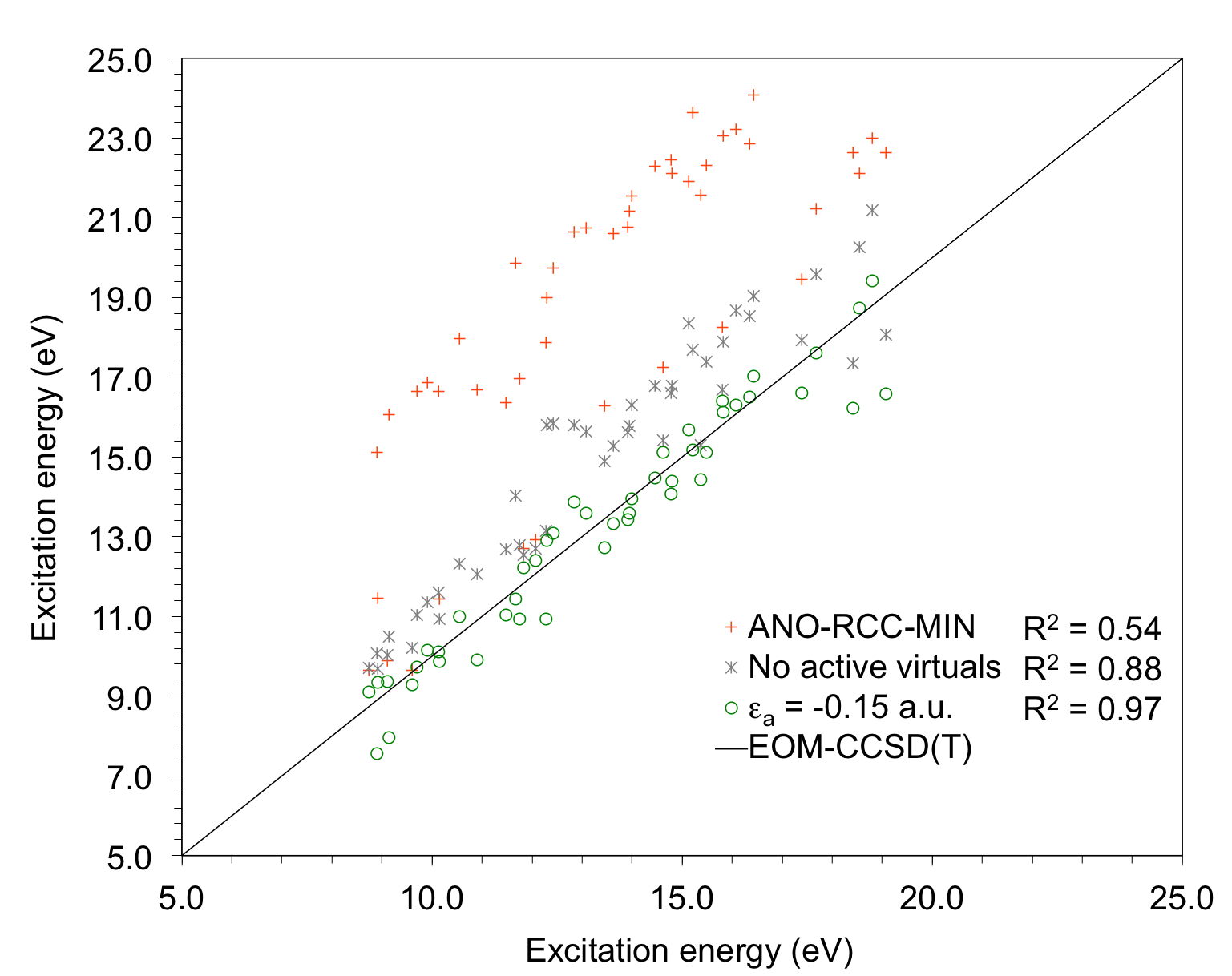
Figure 3: Correlation plots for excitation energies of the ethylene molecule with the target ANO-RCC-MIN effective Hamiltonian, compared to the excitation energies in the parent cc-pVDZ basis. (Excitation energies computed using EOM-CCSD(T)).

Table 5: Statistical information for correlation plots of the excitation energies of water. $R^{2}$ and RMSD values.

Method	$R^{2}$	RMSD (eV)	Average deviations (eV)
			Signed	Unsigned
Parent=DZ
Bare $H$ ANO-RCC-MIN	0.77	6.72	-6.31	6.31
$\bar{H}$ ANO-RCC-MIN no active	0.65	10.36	-9.92	9.92
$\bar{H}$ ANO-RCC-MIN $\bar{\epsilon}_{a}=$HOMO	0.97	1.79	-1.34	1.35
$\bar{H}$ ANO-RCC-MIN $\bar{\epsilon}_{a}=-0.30$	0.99	1.05	-0.07	0.75
Parent=TZ
Bare $H$ ANO-RCC-MIN	0.68	7.43	-6.53	6.53
$\bar{H}$ ANO-RCC-MIN no active	0.55	12.12	-11.17	11.17
$\bar{H}$ ANO-RCC-MIN $\bar{\epsilon}_{a}=$HOMO	0.88	3.56	-2.37	2.46
$\bar{H}$ ANO-RCC-MIN $\bar{\epsilon}_{a}=-0.30$	0.95	2.15	-0.02	1.77

Table 6: Statistical information for correlation plots of the excitation energies of nitrogen, $R^{2}$ and RMSD values.

Method	$R^{2}$	RMSD (eV)	Average deviations (eV)
			Signed	Unsigned
Parent=DZ
Bare $H$ ANO-RCC-MIN	0.97	1.24	-0.61	0.89
$\bar{H}$ ANO-RCC-MIN no active	0.84	4.13	-3.85	3.85
$\bar{H}$ ANO-RCC-MIN $\bar{\epsilon}_{a}=$HOMO	0.97	1.52	-1.17	1.17
$\bar{H}$ ANO-RCC-MIN $\bar{\epsilon}_{a}=-0.30$	0.97	1.01	-0.94	.0.94
Parent=TZ
Bare $H$ ANO-RCC-MIN	0.94	1.31	-0.54	0.99
$\bar{H}$ ANO-RCC-MIN no active	0.80	4.43	-4.25	4.25
$\bar{H}$ ANO-RCC-MIN $\bar{\epsilon}_{a}=$HOMO	0.98	0.99	-0.80	0.80
$\bar{H}$ ANO-RCC-MIN $\bar{\epsilon}_{a}=-0.30$	0.98	0.95	-0.75	0.77

3.3 Potential energy curves

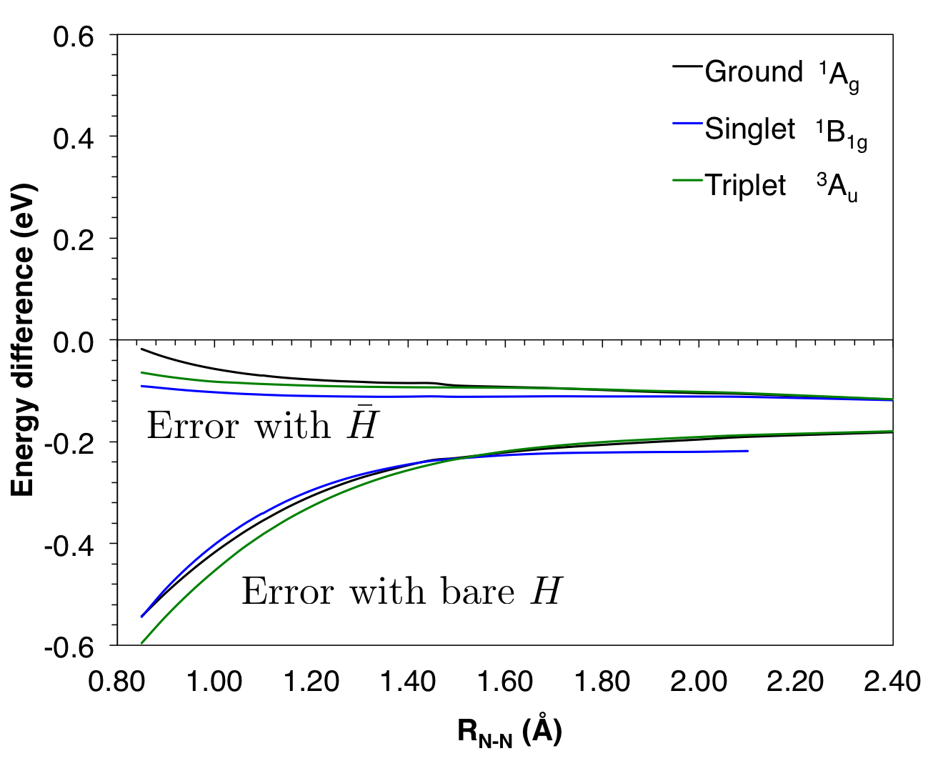
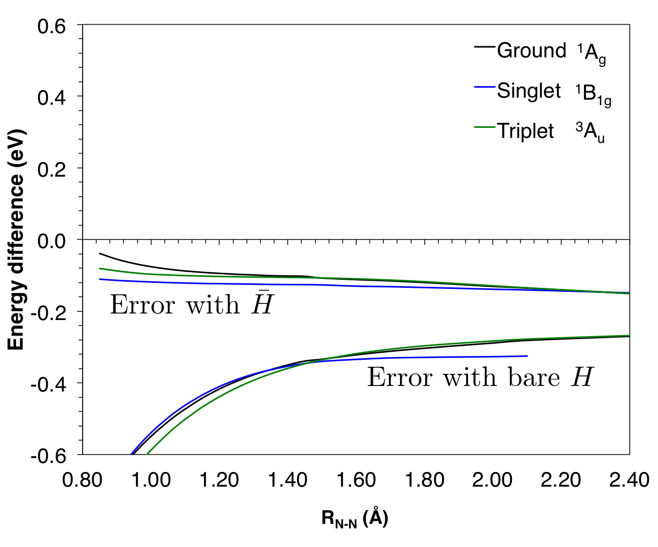
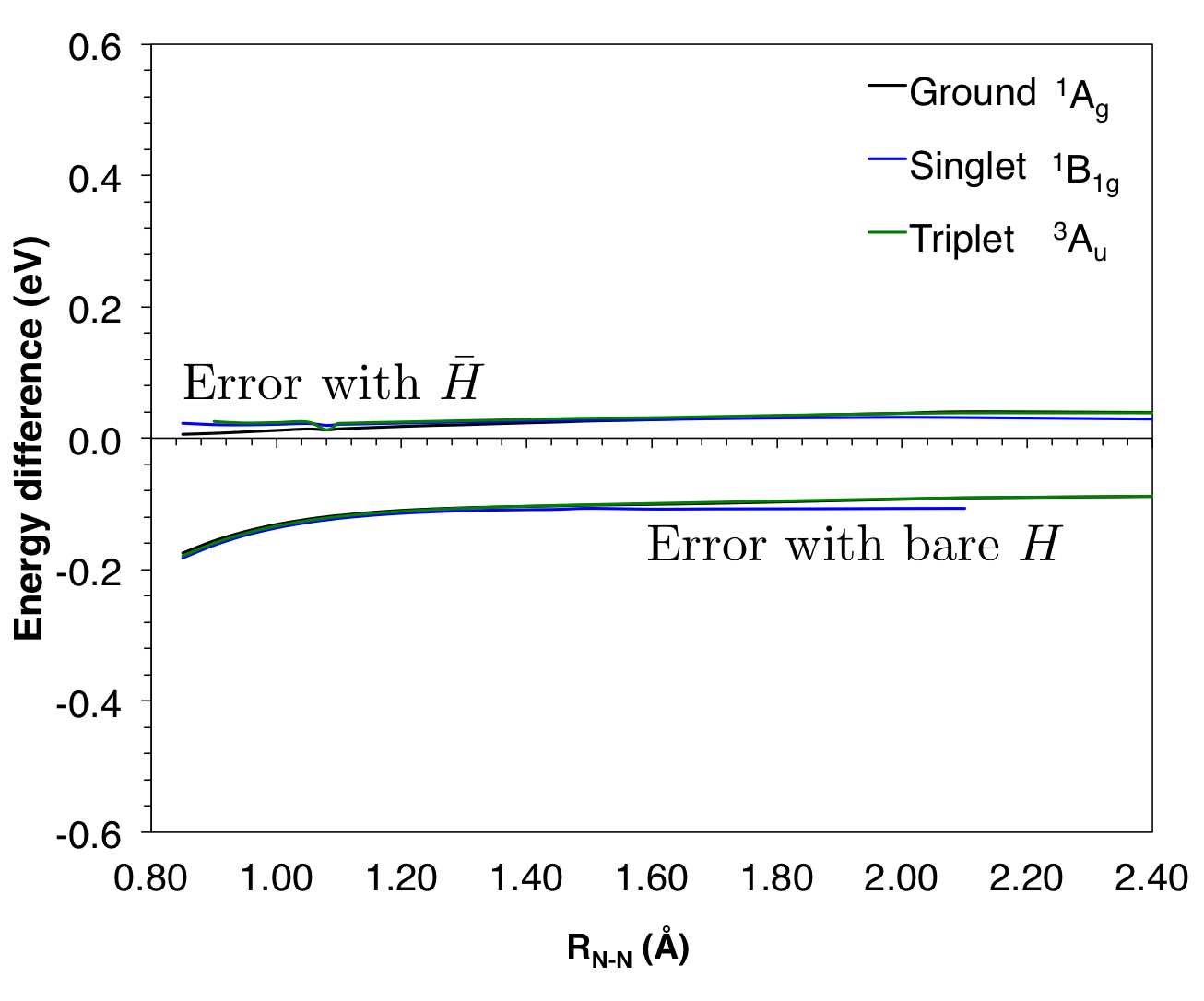
Figure 4: Parallelity errors in the ground, first singlet excited, and first triplet excited state using the bare Hamiltonian $H$ and the effective Hamiltonian $\bar{H}$. The curves are generated using CASSCF(6,6)+CTSD. Top: parent basis=cc-pVDZ, left: target basis=ANO-RCC-MIN, right: target basis=ANO-RCC-MIN, Bottom: parent basis=cc-pVTZ, target basis=cc-pVDZ. The reference basis for each figure is the parent basis.

As a further test of our effective Hamiltonians, we now study how they perform in describing potential energy curves in a minimal (or small) basis. We first consider the nitrogen dimer. In Figure 4 we show the errors in the ground, first singlet excited, and first triplet excited state potential energy curves computed by diagonalizing the effective Hamiltonian in the ANO-RCC-MIN basis, as compared to the parent basis. (The effective Hamiltonian is derived for the singlet ground-state). For comparison we also show errors of the curves computed using the bare Hamiltonian in the ANO-RCC-MIN basis. For each basis, the curves were computed using full valence complete active space self-consistent field followed by a canonical transformation with singles and doubles excitations dynamic correlation treatment (CASSCF+CTSD).

As expected, the bare Hamiltonian potential curves in the minimal basis display very large errors in the compressed bond region, due to the lack of a second shell to describe polarizing effects. In contrast, the effective Hamiltonian yields much smaller errors across the curve (roughly half the error at long bond-lengths, and much higher accuracy at short bond lengths). But more importantly, the errors are very parallel across the entire range of bond-lengths, and consistent between all the states.

As a more challenging probe of the quality of the chemistry that can be described by two-particle Hamiltonians in a minimal basis, we now consider the chromium dimer binding curve. The chromium dimer has been the subject of numerous quantum chemical studies due to the difficulties in obtaining a potential curve of even qualitatively correct shape ^{46, 47, 48, 49}. It is well known that, in addition to the strong correlation arising from the spin coupling of the chromium d electrons, very large basis sets are needed ^{50, 49}. Thus constructing a two-particle effective Hamiltonian for a minimal basis description is a serious challenge.

As a parent basis, we used high quality ANO-RCC bases of double-$\zeta$, triple-$\zeta$, quadruple-$\zeta$ quality ³⁰ supplemented with an additional set of $d$-functions taken from the next $\zeta$ in the series. This yields the following basis set labels and structure: ANO-RCC-DZP+$d$ (21s15p10d6f/5s3p3d1f), ANO-RCC-TZP+$d$ (21s15p10d6f4g/6s4p4d2f1g), and ANO-RCC-QZP+$d$ (21s15p10d6f4g2h/7s5p5d3f2g1h). We used the valence (12,12) active space in the CASSCF calculation. We first tried folding to a target ANO-RCC-MIN (21s15p10d/4s2p1d) basis. While this yielded a bound potential, the binding energy was $111.4$ kcal mol^-1 ($4.83$ eV), several times too large, showing that, at least using our procedure, a reasonable effective two-particle Hamiltonian in a strict minimal basis cannot be constructed. We next tried folding to a slightly larger ANO-RCC-MIN+$d$ basis, where an additional d shell (taken from the double-$\zeta$ basis (21s15p10d/4s2p2d)) was included in the target basis to capture polarization effects. The CASSCF density matrix was used in the $(1,2)$ construction of $\bar{H}$ as the Hartree-Fock potential energy surface has an inconvenient curve crossing.

The experimental curve is shown in Fig 5. The bare Hamiltonian ANO-RCC-MIN+$d$ basis results are shown using CASSCF(12,12) and CASSCF(12,12) plus CTSD. Neither of these curves show any binding, as expected in a minimal basis. We see, however, that the CTSD calculations with the effective Hamiltonian in the ANO-RCC-MIN+$d$ basis yield a nicely bound potential energy curve of a very similar shape and depth to experiment!

The values for the binding energy, equilibrium distance, and spectroscopic constants, obtained using the aforementioned constructed ANO-RCC parent bases, DZP+$d$, TZP+$d$, QZP+$d$, and the target ANO-RCC-MIN+$d$ basis, are given in Table 7. Even using the ANO-RCC-DZP+$d$ external basis we recover binding in the effective ANO-RCC-MIN+$d$ Hamiltonian. Folding down from the largest QZ parent basis, we obtain for our effective ANO-RCC-MIN+$d$ Hamiltonian an R_eq of $1.83$ Å and $D_{e}$ of $1.70$ eV. This compares quite favorably with experiment. Overall, this shows that it is possible to construct an effective Hamiltonian to describe even this very difficult case of the binding of the chromium dimer, so long as the minimal basis is slightly expanded. We understand this because the minimal basis for Cr₂ with a (12,12) active space does not leave any virtual orbitals to be used in a correlated calculation after the folding procedure. In this strongly correlated system, the role of the extra set of d-functions is to give 10 virtual orbitals outside the active space that help to relax the orbitals.

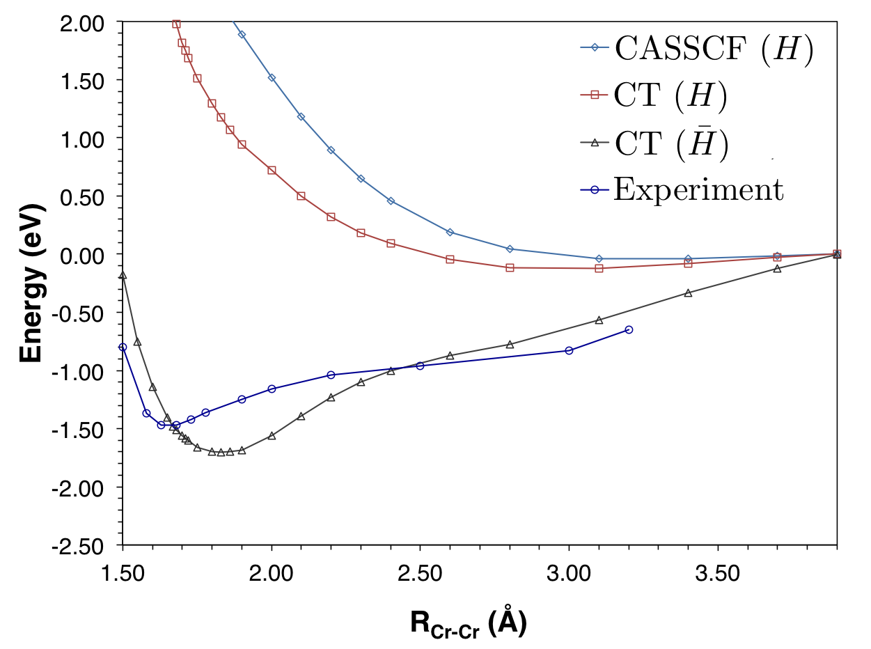
Figure 5: Potential energy curves for the chromium dimer for the different methods shown using the ANO-RCC-MIN+$d$ basis set. External basis set is ANO-RCC-QZP+$d$.

Table 7: Equilibrium bond distances and dissociation energies for the chromium dimer using an effective Hamiltonian in a minimal + $d$ basis, folded down from increasingly large basis sets (DZP, TZP, QZP), and for different values of the active virtual energy $\bar{\epsilon}_{a}$.

Basis	Req (Å)	$D_{e}$ (eV)
MIN+$d$ (DZP+$d$)
$\bar{\epsilon}_{a}$=0.00	2.20	1.55
$\bar{\epsilon}_{a}$=0.05	2.10	1.66
$\bar{\epsilon}_{a}$=0.10	1.90	1.84
MIN+$d$ (TZP+$d$)
$\bar{\epsilon}_{a}$=0.00	2.40	0.75
$\bar{\epsilon}_{a}$=0.04	2.40	0.78
$\bar{\epsilon}_{a}$=0.05	2.40	0.79
MIN+$d$ (QZP+$d$)
$\bar{\epsilon}_{a}$=0.00	1.83	1.70
Experiment	1.679a	1.47b
		1.45c
		1.56d

• Ref. ⁵¹

• Ref. ⁵²

• Ref. ⁵³

• Ref. ⁵⁴

4 Conclusions

In this work we asked whether a simple canonical transformation, using a single-reference-like modified second-order perturbation theory formula, yields an effective Hamiltonian in a minimal (or very small) basis with qualitatively correct chemistry. As we saw, the answer is in the affirmative: such minimal basis set effective Hamiltonians give qualitatively correct excitation energies and binding curves in water, nitrogen, ethylene, and even the chromium dimer!

Effective Hamiltonians formally provide a conceptual link between quantitative and qualitative reasoning. The simple nature of the construction here means that we can now derive accurate effective Hamiltonians for complex systems in practice, including systems with transition metals, and for correlated electrons in the condensed phase, where models are essential not only for interpretation but for practical computation. Intriguingly, our various calculations suggests that these simple effective Hamiltonians may even be quantitatively accurate. The technique here thus further provides the possibility of very low cost (that is lower than multireference perturbation theory) treatment of dynamic correlation in challenging multireference quantum chemistry.

References

- Polyansky et al. 2003 Polyansky, O. L.; Császár, A. G.; Shirin, S. V.; Zobov, N. F.; Barletta, P.; Tennyson, J.; Schwenke, D. W.; Knowles, P. J. Science 2003, 299, 539–542
- Karton et al. 2006 Karton, A.; Rabinovich, E.; Martin, J. M.; Ruscic, B. The Journal of chemical physics 2006, 125, 144108
- Tajti et al. 2004 Tajti, A.; Szalay, P. G.; Császár, A. G.; Kállay, M.; Gauss, J.; Valeev, E. F.; Flowers, B. A.; Vázquez, J.; Stanton, J. F. The Journal of chemical physics 2004, 121, 11599–11613
- Sharma et al. 2014 Sharma, S.; Yanai, T.; Booth, G. H.; Umrigar, C.; Chan, G. K.-L. The Journal of chemical physics 2014, 140, 104112
- Yang et al. 2014 Yang, J.; Hu, W.; Usvyat, D.; Matthews, D.; Schütz, M.; Chan, G. K.-L. Science 2014, 345, 640–643
- Blaizot and Ripka 1986 Blaizot, J.-P.; Ripka, G. Quantum theory of finite systems; Mit Press Cambridge, 1986; Vol. 3
- Onida et al. 2002 Onida, G.; Reining, L.; Rubio, A. Reviews of Modern Physics 2002, 74, 601
- Werner and Millis 2010 Werner, P.; Millis, A. J. Physical review letters 2010, 104, 146401
- Kemble 1937 Kemble, E. C. The fundamental principles of quantum mechanics; Dover, 1937
- Brandow 1967 Brandow, B. H. Reviews of Modern Physics 1967, 39, 771
- Westhaus 1973 Westhaus, P. International Journal of Quantum Chemistry 1973, 7, 463–477
- Freed 1974 Freed, K. F. The Journal of Chemical Physics 1974, 60, 1765–1788
- Iwata and Freed 1976 Iwata, S.; Freed, K. F. The Journal of Chemical Physics 1976, 65, 1071–1088
- Durand and Malrieu 2009 Durand, P.; Malrieu, J.-P. Advances in chemical Physics 2009, 321–412
- Wegner 1994 Wegner, F. Annalen der physik 1994, 506, 77–91
- Głazek and Wilson 1993 Głazek, S. D.; Wilson, K. G. Physical Review D 1993, 48, 5863
- White 2002 White, S. R. The Journal of chemical physics 2002, 117, 7472–7482
- Bartlett and Musiał 2007 Bartlett, R. J.; Musiał, M. Reviews of Modern Physics 2007, 79, 291
- Stanton and Bartlett 1993 Stanton, J. F.; Bartlett, R. J. The Journal of chemical physics 1993, 98, 7029–7039
- Lyakh et al. 2011 Lyakh, D. I.; Musiał, M.; Lotrich, V. F.; Bartlett, R. J. Chemical reviews 2011, 112, 182–243
- Yanai and Chan 2006 Yanai, T.; Chan, G. K.-L. The Journal of chemical physics 2006, 124, 194106
- Yanai and Chan 2007 Yanai, T.; Chan, G. K.-L. The Journal of chemical physics 2007, 127, 104107
- Neuscamman et al. 2010 Neuscamman, E.; Yanai, T.; Chan, G. K.-L. The Journal of chemical physics 2010, 132, 024106
- Neuscamman et al. 2010 Neuscamman, E.; Yanai, T.; Chan, G. K.-L. International Reviews in Physical Chemistry 2010, 29, 231–271
- Mazziotti 2006 Mazziotti, D. A. Physical review letters 2006, 97, 143002
- Mazziotti 2007 Mazziotti, D. A. Physical Review A 2007, 75, 022505
- Evangelista 2014 Evangelista, F. A. arXiv preprint arXiv:1406.0114 2014,
- Yanai and Shiozaki 2012 Yanai, T.; Shiozaki, T. The Journal of chemical physics 2012, 136, 084107
- Valeev 2004 Valeev, E. F. Chemical physics letters 2004, 395, 190–195
- Roos et al. 2005 Roos, B. O.; Lindh, R.; Malmqvist, P.-Å.; Veryazov, V.; Widmark, P.-O. The Journal of Physical Chemistry A 2005, 109, 6575–6579
- Dunning 1989 Dunning, T. H. The Journal of chemical physics 1989, 90, 1007
- Kutzelnigg 1979 Kutzelnigg, W. Chemical Physics Letters 1979, 64, 383–387
- Neuscamman et al. 2009 Neuscamman, E.; Yanai, T.; Chan, G. K.-L. The Journal of chemical physics 2009, 130, 124102
- Kutzelnigg and Mukherjee 1997 Kutzelnigg, W.; Mukherjee, D. The Journal of chemical physics 1997, 107, 432–449
- Mazziotti 1998 Mazziotti, D. A. Chemical physics letters 1998, 289, 419–427
- Mazziotti 1998 Mazziotti, D. A. Physical Review A 1998, 57, 4219
- Kutzelnigg and Mukherjee 1999 Kutzelnigg, W.; Mukherjee, D. Journal of Chemical Physics 1999, 110, 2800–2809
- Shamasundar 2009 Shamasundar, K. The Journal of chemical physics 2009, 131, 174109
- Banerjee and Simons 1981 Banerjee, A.; Simons, J. International Journal of Quantum Chemistry 1981, 19, 207–216
- Evangelista and Gauss 2011 Evangelista, F. A.; Gauss, J. The Journal of chemical physics 2011, 134, 114102
- Hanauer and Köhn 2011 Hanauer, M.; Köhn, A. The Journal of chemical physics 2011, 134, 204111
- Datta et al. 2011 Datta, D.; Kong, L.; Nooijen, M. The Journal of chemical physics 2011, 134, 214116
- Ten-No 2004 Ten-No, S. The Journal of chemical physics 2004, 121, 117–129
- Kedžuch et al. 2005 Kedžuch, S.; Milko, M.; Noga, J. International journal of quantum chemistry 2005, 105, 929–936
- Kendall et al. 1992 Kendall, R. A.; Dunning Jr, T. H.; Harrison, R. J. The Journal of chemical physics 1992, 96, 6796–6806
- Roos and Andersson 1995 Roos, B. O.; Andersson, K. Chemical physics letters 1995, 245, 215–223
- Dachsel et al. 1999 Dachsel, H.; Harrison, R. J.; Dixon, D. A. The Journal of Physical Chemistry A 1999, 103, 152–155
- Celani et al. 2004 Celani, P.; Stoll, H.; Werner, H.-J.; Knowles, P. Molecular Physics 2004, 102, 2369–2379
- Kurashige and Yanai 2011 Kurashige, Y.; Yanai, T. The Journal of chemical physics 2011, 135, 094104
- Roos 2003 Roos, B. O. Collection of Czechoslovak chemical communications 2003, 68, 265–274
- Bondybey and English 1983 Bondybey, V.; English, J. Chemical Physics Letters 1983, 94, 443–447
- Casey and Leopold 1993 Casey, S. M.; Leopold, D. G. The Journal of Physical Chemistry 1993, 97, 816–830
- Hilpert and Ruthardt 1989 Hilpert, K.; Ruthardt, K. Ber. Bunsenges. 1989, 93, 1070–1078
- Su et al. 1993 Su, C.-X.; Hales, D. A.; Armentrout, P. Chemical physics letters 1993, 201, 199–204