From graphs to signals and back: Identification of network structures using spectral analysis

Abstract

The structure of networks describing interactions between entities gives significant insights about how these systems work. Recently, an approach has been proposed to transform a graph into a collection of signals, using a multidimensional scaling technique on a distance matrix representing relations between vertices of the graph as points in a Euclidean space: coordinates are interpreted as components, or signals, indexed by the vertices. In this article, we propose several extensions to this approach: We first extend the current methodology, enabling us to highlight connections between properties of the collection of signals and graph structures, such as communities, regularity or randomness, as well as combinations of those. A robust inverse transformation method is next described, taking into account possible changes in the signals compared to original ones. This technique uses, in addition to the relationships between the points in the Euclidean space, the energy of each signal, coding the different scales of the graph structure. These contributions open up new perspectives by enabling processing of graphs through the processing of the corresponding collection of signals. A technique of denoising of a graph by filtering of the corresponding signals is then described, suggesting considerable potential of the approach.

1 Introduction

The development of data processing methods is crucial with the recent explosion of data made possible by technological devices. Many systems, previously inaccessible by traditional methods of quantitative analysis by lack of information, are now described by huge amounts of data, so that the limiting factor is now the absence of tools to give them sense. Among these systems, many can be represented as networks i.e., a set of relationships between entities. Network theory [33] has been developed to supply toolboxes, such as for detecting communities [15], in order to understand the underlying properties of these systems, with many successes. More recently, connections between signal processing and networks theory have tremendously increased. The field of signal processing over networks has been extensively studied in recent years [43] with the objective to transpose concepts developed in classical signal processing, such as Fourier transform or wavelets, in the graph domain. These works, based on spectral graph theory [10], have led to a growing set of significant results, among them filtering of graph signals (i.e., signals defined over a graph) [43, 40], spectral wavelets [20], wavelet filterbanks [32, 43, 39, 34] vertex-frequency analysis [44] of graphs signals, multiscale community mining using graph wavelets [46], or sampling for graph signals [4, 8, 30, 16, 47] added to considerations about uncertainty principle on graphs [1, 37, 48].

For the study of networks themselves, another approach linked to signal processing has been considered: it consists in a duality between graphs and signals, based on the transformation of graphs into signals and reciprocally, in order to take advantage of both signal processing and graph theory. With the development of the network science [33], some works have proposed to map time series into graph objects, aiming at using the wide range of measures and tools defined on networks to highlight properties in the time domain; this approach has been successfully used in the analysis of nonlinear time series [7, 35], in the characterization of nonlinear dynamics [52, 42, 13] or in the identification of invariant structures [12], with significant results in applications such as heart rate [7] or earthquake [2] analyses.

Conversely, mapping a graph into time series has been less intensively studied. Recently, Weng et al. [51] proposed to explore the structure of scale-free networks using finite-memory random walks, where the values of time series at time $t$ are the degree of the vertex visited by the walker at step $t$. The resulting time series, obtained from different real-world networks, exhibit correlations, linked with the scale-free property of these networks. With a similar approach, Campanharo et al. [7] proposed a random walk based algorithm to map graphs into time series by associating a specific value in the time domain with vertices, with the particularity that the graphs are themselves derived from time series. Girault et al. [17] extended this approach in the case where the graph is the object of interest, by using semi-supervised learning to map vertices to signal magnitudes such that the resulting time series are smooth. Using an alternative approach, Haraguchi et al. [26] and later Shimada et al. [41] proposed a deterministic method based on classical multidimensional scaling (CMDS) to represent the vertices of the graph as a set of points in a Euclidean space, where the relations described by the edges are represented by distances between points.

An attractive feature of this latter approach, in comparison with random walks, is that it is fully deterministic since for a given graph, its representation in the signal domain remains the same. A second interesting point is that all information is included in the signals: from them, it is possible, under some assumptions, to compute exactly the original graph. Our contribution in this article elaborates on preliminary contributions along this line in [21], and extends the method proposed in [41] on several points: in Section 2, the methodology is examined more deeply, and application of the method to a wider variety of graph structures is studied through illustrations. A robust inverse transformation is then proposed in Section 3 to transform back a collection of signals to a graph, with a focus on the case where the collection of signals is degraded and is not anymore the direct result of the transformation of a graph. Finally, we develop a comprehensive framework in Section 4 to analyze graphs using tools from signal processing, namely spectral analysis, with an illustration to the denoising of a graph. Note that the present work focuses on static graphs; in previous works, some applications of the present framework have been proposed to study and extract the topology of dynamic graphs [23, 22, 24].

Notations

Throughout the article, the following notations are adopted. Let $\mathcal{G}=(\mathcal{V},\mathcal{E})$ be a simple undirected and unweighted graph, where $\mathcal{V}$ is the set of vertices of size $n$ and $\mathcal{E}$ the set of edges of size $m$. We note $\bm{A}$ its adjacency matrix, whose element $a_{ij}$ is equal to $1$ if $(i,j)\in\mathcal{E}$, $0$ otherwise, and for $i,j\in\mathcal{V}$. The terms “signals” or “components” are indistinctly used in the following, while avoiding the term time series, to prevent the confusion with the case of dynamic graphs.

2 From graph to signals

2.1 Transformation using multidimensional scaling

Shimada et al. [41] proposed a method to transform a graph with $n$ vertices into a collection of signals of $n$ points indexed by the vertices of the graph by using multidimensional scaling (MDS) [6].

MDS is a set of mathematical techniques used to represent dissimilarities among pairs of objects as distances between points in a multidimensional space whose dimension is low. Classical MDS (CMDS) is a particular case of metric MDS where the dissimilarities are assumed to be Euclidean distances. The matrix $\bm{X}$ of coordinates in the low-dimensional space can be computed analytically: Starting with a distance matrix $\bm{\Delta}=(\delta_{ij})_{i,j=1,..,n}$, we first compute a double centering of the matrix whose terms are squared: $\bm{B}=-\frac{1}{2}\bm{J}\bm{\Delta}^{(2)}\bm{J}$ with $\bm{\Delta}^{(2)}=\bm{\Delta}\circ\bm{\Delta}$ and $\bm{J}=\bm{I}_{n}-\frac{1}{n}\bm{1}_{n}\bm{1}_{n}^{T}$ where $\bm{I}_{n}$ is the identity matrix , $\bm{1}_{n}\bm{1}_{n}^{T}$ a $n\times n$ matrix of ones, and $\circ$ the Hadamard product. The CMDS solution is given by $\bm{X}=\bm{Q}_{+}\bm{\Lambda}_{+}^{\frac{1}{2}}$ with $\bm{\Lambda_{+}}$ a diagonal matrix whose terms are the strictly positive eigenvalues of the matrix $\bm{B}$ sorted in an increasing order and $\bm{Q_{+}}$ is the matrix of the corresponding eigenvectors. The resulting signals are the components (or columns) of the matrix $\bm{X}$. The $j$-th signal is noted $\bm{X}^{(j)}$. An alternative approach to find the matrix $\bm{X}$ consists in solving the following optimization problem: $\min_{\bm{X}}{L(\bm{X}})=\sum_{i<j}^{n}(\delta_{ij}-d_{ij}(\bm{X}))^{2}$ where $d_{ij}(\bm{X})$ is the Euclidean distance between the points $i$ and $j$. An algorithm called SMACOF [6] has been developed to solve such problem. It is worth to note that the solution is not unique, as any rotation, reflection or translation of points in the Euclidean space will preserve the distances.

In [41], CMDS is used to transform a graph into signals by projecting vertices of the graph in a Euclidean space, such that distances between these points correspond to relations in the graph. A distance matrix between the vertices of the graph $\bm{\Delta}$ describes these relations: Shimada et al. proposed the following definition from the adjacency matrix $\bm{A}$ for the distance matrix:

$$\bm{\Delta}=\bm{A}+w(\bm{1}_{n}\bm{1}_{n}^{T}-\bm{I}_{n}-\bm{A})$$ (1)

where $w$ is an arbitrary weight strictly greater than $1$. This definition does not include a notion of proximity between vertices, beyond direct linkage: if the two vertices are connected, the distance is equal to $1$, otherwise it is equal to $w$. The remoteness between two vertices, which can be measured using for instance the length of the shortest path between the two vertices, is not taken into account in this definition: two pairs of unlinked vertices will have a distance equal to $w$, whether they are close or not in the graph. One of the advantage of this distance matrix, unlike a distance matrix based for instance on the length of the shortest path between the vertices, is that it is Euclidean (under some assumptions on the value of $w$, as discussed later in the paper), and then there exists an exact solution. Furthermore, the information about the proximity in the graph is no more induced from the graph, but is automatically retrieved by the algorithm: if the considered Euclidean space is low-dimensional, the distances cannot be well-preserved and only the distances representing distant vertices will be respected. This enables us to look at, component by component, how this approximation is performed, i.e., which vertices are roughly considered as neighbors.

For a given distance matrix, it does not exist necessarily a configuration of points $\bm{X}$ such that distances between these points are equal to distances defined in the distance matrix. In the case where the distance matrix $\bm{\Delta}$ is defined by Equation 1, the structure of the graph as well as the parameter $w$ has an influence on the existence of a solution $\bm{X}$. This influence has been barely studied in [26] and [41]. In [26], the authors compare for different values of $w$ the quality of the reconstruction on several graphs generated using the Watts-Strogatz model and two real-world networks, by the comparison of their edges sets. They conclude that the value $w$ should reside between $1$ (excluded) and $1.01$. The same kind of approach is followed in [41], but restricted to Watts-Strogatz model where the probability of rewiring varies from $0.01$ to $1$. Their conclusion is that for $n=400$, $w$ should be comprised between $1$ (excluded) and $1.14$, and that this upper bound depends on the value of $n$ and should be as close to unity as possible, without substantial argument for that. We propose in the following an upper bound for the value of $w$ to guarantee that the matrix $\bm{\Delta}$ is Euclidean, i.e., there exists a configuration $\bm{X}$ such that the Euclidean distances between points are equal to $\bm{\Delta}$. The calculation of this upper bound relies on the positive-semidefiniteness of the resulting matrix $\bm{B}$, which is the covariance matrix of $\bm{X}$: $\bm{B}=\bm{X}\bm{X}^{T}$. The study of the eigenvalues of $\bm{B}$ according to $w$ and the adjacency matrix $\bm{A}$, detailed in A, gives an upper bound for $w$: $w\leq\sqrt{\frac{n}{n-2}}$ with $n$ the number of vertices. This result agrees with the partial results obtained in [26] and [41]: $w$ should be close to $1$, all the greater given the number of vertices $n$. In addition, in practice setting $w$ below this upper bound is not required for most graphs, although it ensures that the matrix $\bm{\Delta}$ will stay Euclidean, even with a peculiar topology of the graph.

Alternative distance matrix could be used instead of the one proposed in [41]. As described previously, a natural measure of closeness between two vertices in a graph is the length of the shortest path between the vertices [45]. Distances also based on similarity between adjacent vertex sets are worth considering. These two alternative dissimilarities have the advantage to be easily extended to the case where the graph is weighted i.e., each edge has a weight giving its importance. There also exist alternative methods to CMDS to transform graph into points in a Euclidean space. For instance, the method of Laplacian eigenmaps, proposed by Belkin et al. [5], have been used in a context of dimensionality reduction and data representation, and is based on a diagonalization of the Laplacian matrix of the graph. Many parallels can be done between the two approaches, even if they differ on the final representation of vertices in the Euclidean space [38]. Such a comparison is beyond the scope of this article and will not be discussed further here.

2.2 Graph models and theoretical results

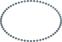
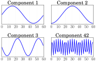
(a) $2$-ring lattice with $60$ vertices (2RL-60-10)

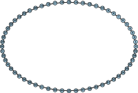
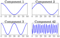
(b) $10$-ring lattice with $60$ vertices (RL-60-2)

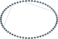
(c) Watts-Strogatz model with $60$ vertices, $k=2$ and $p=0.1$ (WS60-2-.1)

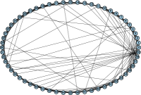
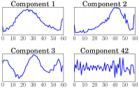
(d) Watts-Strogatz model with $60$ vertices, $k=10$ and $p=0.1$ (WS60-10-.1)

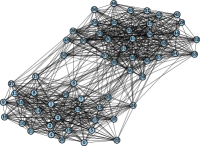
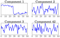
(e) Stochastic block model with 2 communities, $60$ vertices, $p_{w}=0.7$ and $p_{b}=0.1$ (SBM60-2)

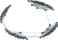
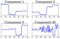
(f) Stochastic block model with 4 communities, $60$ vertices, $p_{w}=0.9$ and $p_{b}=0.01$ (SBM60-4)

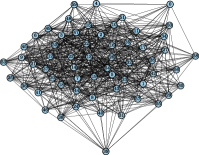
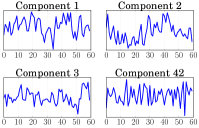
(g) Erdös-Rényi model with $60$ vertices and $p=0.4$ (ER60-.4)

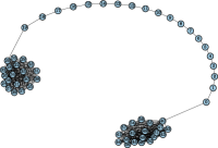
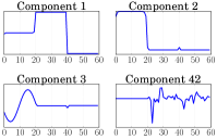
(h) Barbell model with two cliques of $20$ vertices and a path between them of $20$ vertices (BAR60)

Figure 1: Illustrations on several instances of graph models of the transformation of a graph into a collection of signals. All graphs have $n=60$ vertices. For each sub-figure, the left plot shows a two-dimensional representation of the graph, while the right plot displays the first three components, with high energies, and the arbitrarily chosen component 42, a low-energy component.

This section introduces models that will be used to generate illustrations of the method throughout the article, as well as theoretical results associated to these models.

$k$-ring lattices

A $k$-ring lattice is a graph where each vertex $i$ is connected to the vertices $\{i-\frac{k}{2},i-\frac{k}{2}+1,\ldots,i-1,i+1,\ldots,i+\frac{k}{2}-1,i+\frac{k}{2}\}$, for $k\in\{2,4,\ldots,n\}$. As Shimada et al. discussed in [41], it is immediate to find expected eigenvalues and eigenvectors in this case using circulant matrix theory [19].

The computation of eigenvalues of $\bm{B}$ leads to

$$\lambda_{q}=\frac{\alpha}{2n}\sum_{j=0}^{n-1}{\zeta^{jq}}-\frac{1}{2}\left(\sum_{j=1}^{\frac{k}{2}}\zeta^{jq}+\sum_{j=n-\frac{k}{2}}^{n-1}\zeta^{jq}+w^{2}\sum_{j=\frac{k}{2}+1}^{n-\frac{k}{2}-1}\zeta^{jq}\right)$$ (2)

where $\alpha=k+(n-1-k)w^{2}$ and $\zeta=e^{\frac{2i\pi}{n}}$ is the $n$th root of the unity. The eigenvectors are given by the columns of the Fourier matrix. Details of the calculation are given in B.

When the eigenvalues are ordered by the value of $q$, the eigenvectors are considered in increasing order of frequencies. The components are however sorted according to the energy of eigenvalues $\lambda_{k}$ when applying CMDS, which correspond to the sorting according to the value of $q$ only when $k=2$. In this case, the resulting signals are then harmonic oscillations whose frequencies increase as lower-energy components are considered. When $k$ increases, the components are no longer sorted by frequencies.

Watts-Strogatz model

The Watts-Strogatz model [50] has been developed to build graphs with small-world property, where the average length of the shortest paths between vertices is low compared to the number of vertices, while the clustering coefficient is high. This property has been highlighted in many systems, such as for instance social networks. From a $k$-ring lattice, each edge $(u,v)$ is rewired with probability $p$ to become $(u,w)$, where $w$ is uniformly chosen among other vertices. Shimada et al. give a second-order approximation of the expected eigenvalues and eigenvectors according to the probability $p$, using perturbation theory. They showed that the correlation between the approximation and the actual signals is high when $p$ is low, and decreases when $p$ increases, which is consistent with intuition.

Erdös-Rényi model

A random graph is a graph whose set $\mathcal{V}$ of vertices is fixed and links between these vertices are drawn randomly [14]. Random matrix theory suggests that eigenvectors are random vectors in $\mathbb{R}^{n}$, naturally conjectured to be distributed as i.i.d. Gaussian vectors [11]. As for eigenvalues, the Wigner results [49] show that the maximal eigenvalue is comprised between $np(1-\frac{1}{\sqrt{n}})$ and $np(1+\frac{1}{\sqrt{n}})$ while the remaining eigenvalues follow a semicircle law on the interval $[-\frac{1}{\sqrt{n}},\frac{1}{\sqrt{n}}]$, giving the energies of signals.

Stochastic block model

A simple stochastic block model [29] is used to generate a graph with communities. Each of the $n$ vertices is assigned to one of the $K$ communities, and edges between each pair of vertices is randomly and independently drawn according to probabilities depending on the group of vertices: if the two vertices belong to the same community, the probability, noted $p_{w}$, is close to $1$ while otherwise, the probability between vertices of different groups, noted $p_{b}$, is lower. The settings of $p_{w}$ and $p_{b}$ lead to customized density of edges within and between communities. In [31], intuitions about the shape of the signals are given, in an application of segmentation of images. They suggest that the eigenvectors of block matrices are piecewise constant with respect to the communities.

Barbell model

The barbell model [3] is defined as two cliques, each containing $n_{c}$ vertices, linked by a path with $n_{p}$ vertices. Based on the results defined previously, the shape of the eigenvectors is expected to be close to the ones in the case of stochastic block model, since each clique is community, as well as to the ones in the $2$-regular lattices, which is encountered in the path part of the graph.

2.3 Illustrations

Figure 1 shows illustrations of the transformation of a graph into a collection of signals, on several instances of graph models introduced in the previous section, all set with $n=60$ vertices. For each sub-figure, the left plot shows a two-dimensional representation of the studied graph, while the right plot displays the first three components, with high energies, and the arbitrarily chosen component 42, a low-energy component.

In all cases, the obtained signals are consistent with the expected results described in the previous section. For the $k$-ring lattices (Figure 1a for $k=2$ and Figure 1b for $k=10$), the signals are harmonic oscillations, grouped in pairs of signals with the same frequency and a difference of phase equal to $\frac{\pi}{2}$. For the high-energy components, the value of $k$ does not have any influence. However, the frequency of signals differs, as expected, for lower-energy components, as the sorting of components is guided by the eigenvalues.

When noise is added, here by considering the Watts-Strogatz model with a probability of rewiring equal to $p=0.1$ (Figure 1c for $k=2$ and Figure 1d for $k=10$), the signals are also noisy, as described by Shimada et al. [41]. According to the value of $k$, the consequences of the noise on the shape of the resulting signals differ: for $k=10$, more edges are rewired, but the structure is barely affected since each vertex in linked with its $10$ nearest neighbors: The ring is then preserved, leading to noisy harmonic oscillations. However, when $k=2$, one single rewiring causes the disappearance of the ring: the structure of the graph is then different from a regular lattice, leading to high changes in signals.

Figures 1e and 1f show two instances of the stochastic block model, the first one with two communities with $p_{w}=0.7$ and $p_{b}=0.1$ and the second one with four communities and $p_{w}=0.9$ and $p_{b}=0.01$. An interesting observation is that the high-energy components display the structure of communities, with noisy plateaus corresponding to the dense parts of the graph. It is worth noting that the number of relevant high-energy components is equal to the number of communities in the graph minus one, as one component is sufficient to discriminate two communities. As for the low-energy components, they are noisy signals, corresponding to the structure inside communities. These random structures correspond to a random graph of type Erdös-Rényi, an instance of which is represented in Figure 1g: the resulting signals do not exhibit any structure, only looking as white noise.

Finally, Figure 1h displays an instance of the Barbell model, which combines features obtained for the previous instances: plateaus for the first high-energy components, as highlighted for the stochastic block model, describing the cliques, harmonic oscillation of the third component (only the part which corresponds to a path), found for the $k$-ring lattice, and finally noisy signal for low-energy components, as seen for the Erdös-Rényi model.

These illustrations show the connection between graph structure and the resulting signals after transformation, that will be used in Section 4 to study the topology of the graph using spectral analysis, and to perform standard operations, such as filtering, on graphs. Before that, a study of the inverse transformation is proposed, as it will enable us to represent a collection of signals in the graph domain.

3 Inverse transformation: From signals to graph

3.1 Statement of the problem

Transformation from signals, or time series, to graph has been studied in many applications, as in [7] or [35], in order to use network theory as a tool for the understanding of time series. These methods are nevertheless of no use in our case, because the signals are themselves a representation of a specific graph, hence it can be seen as a restoration problem. Ignoring this would lead to inconsistent results between the represented and the reconstructed graphs. Hence, the inverse transformation shall take into account this knowledge to preserve the original topology of the underlying graph. By construction of the collection of signals $\bm{X}$, the perfect retrieval of the underlying graph is easily reachable, by considering the distances between each point: As built using CMDS, these distances represent the adjacency matrix. However, when $\bm{X}$ is degraded or modified, for instance by filtering (see Section 4.3), the distances are no longer directly the ones computed between vertices, even if they stay in the neighborhood of these distances. It is nevertheless not possible to directly retrieve the comprehensive set of links of the graph. This case is yet worth considering if processing of signals is performed in a goal of analysis: altering the signals will also alter the distances, preventing the direct inverse transformation.

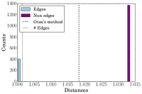
(a)

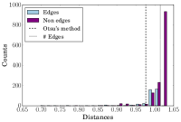
(b)

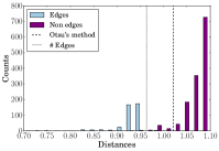
(c)

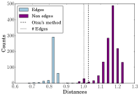
(d)

Figure 2: Inverse transformation from a collection of signals obtained after transformation of an instance of the stochastic block model with four communities (SBM60-4). The figures show the histograms of distances between points $\{d(\bm{X})_{ij}\}_{i,j\in\{1,\ldots,n\}}$ in the Euclidean distances: light blue bars represent distances corresponding to edges while dark purple bars represent distances corresponding to non-edges. The dashed line represents the threshold obtained using Adapted Otsu’s method (see Algorithm 2), while the dotted line represents the threshold obtained using the number of edges of the original graph. The signals are considered either non-degraded or degraded, obtained by removing the lowest-energy component. The computation of distances is performed without or with considering energies of components (a) Non-degraded case and unweighted distances: the distances are either equal to 1 or $w$. Discrimination between edges and non-edges is trivial. (b) Degraded case and unweighted distances: distribution of distances are mixed and no simple thresholding is feasible. (c) Degraded case and weighted distances with $\alpha=2$: the distributions are separated and thresholding is good (d) Degraded-case and weighted distances with $\alpha=4$: the distributions are better separated.

We propose in the following section a robust inverse transformation, based on the thresholding of distances. Two enhancements are discussed to improve the separability of distances. Finally, we discuss two methods of thresholding.

3.2 Robust inverse transformation

The two contributions we propose in the following aim at addressing the drawback raised in the statement of the problem: the two distributions of distances representing edges and non-edges, can overlap when the collection of signals is degraded, preventing an efficient thresholding.

Let us consider a collection of signals $\bm{X}$ with $K$ components. The objective of the inverse transformation is to obtain an adjacency matrix $\tilde{\bm{A}}$, from the distances $\bm{D}(\bm{X})$. This adjacency matrix describes the graph $\tilde{\mathcal{G}}=(\tilde{\mathcal{V}},\tilde{\mathcal{E}})$.

Energy-weighted distances

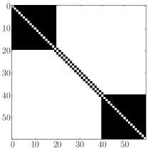
(a) Original adjacency matrix

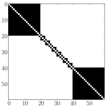
(b) Final adjacency matrix with $K=10$

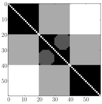
(c) Adjacency matrix after considering the first three components: $\tilde{\bm{A}}=\tilde{\bm{A}}_{1}+\tilde{\bm{A}}_{2}+\tilde{\bm{A}}_{3}$

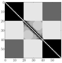
(d) Adjacency matrix before thresholding at Step 6 of Algorithm 1

Figure 3: Illustration of the sequential update of the adjacency matrix to retrieve the underlying graph from a collection of signals. The original graph is an instance of the Barbell model, composed of two cliques of $20$ vertices linked between them by a path of $20$ vertices (BAR60). The collection of signals $\bm{X}$ is degraded by keeping only the first $K=10$ components. The color codes the intensities, from white to black.

An initial observation to improve the distinction between distances representing edges and those representing non-edges is that the energies of components are not taken into account in the processing of the distance matrix $\bm{D}(\bm{X})$. The high-energy components have though a strong influence in the description of the global topology of the graph: If the distance between two vertices $i$ and $j$ in a high-energy component is high, it means that the two vertices are likely to be distant in the graph. Conversely, if the distance in a high-energy component is low, then the two vertices are likely to be connected in the graph. Neglecting the importance of energies of components comes to forget the hierarchy of components in their description of the global structure of the graph. One way to add this information is to compute a distance weighted by the energies of the components: $d(\bm{X})_{ij}=\sqrt{\sum_{k=1}^{K}{e_{k}^{\alpha}(x_{ik}-x_{jk})^{2}}}$ with $\alpha\geq 0$, where $e_{k}$ is the energy of component $k$, computed as $e_{k}=\sum_{i=1}^{n}{x_{ik}^{2}}$, and normalized such that $\sum_{k=1}^{K}e_{k}^{\alpha}=1$. The parameter $\alpha$ controls the importance of the weighting: if $\alpha$ is high, the high-energy components have a higher importance in the computation of distances compared to the low-energy components. Figures 2c and 2d display the distribution of distances representing edges and those representing non-edges, using respectively $\alpha=2$ and $\alpha=4$. Compared with the distributions in Figure 2b, the two distributions are better discriminated when $\alpha$ increases, enabling a better retrieval of the underlying graph. The right choice of $\alpha$ is nevertheless empirical and depends on the collection of signals.

Sequential update of the adjacency matrix

Weighted computation of distances enables the inverse transformation to take into account the energies of components, and produces, as shown in Figure 2, a better separation of distances. Energies of components could be taken into account in another way by considering intermediary adjacency matrices $\tilde{\bm{A}_{k}}$, where $\tilde{\bm{A}_{k}}$ is the adjacency matrix obtained by retaining only the first $k$ components using the method described in the introduction. Thus, these different structures, at different scales, are successively considered: the first components describe the structure at large scale, and adding one-by-one the components increase weights for the less dominating edges. Summing over all these intermediary states is based on the assumption that if an edge exists in the graph, it will be present in many intermediary states. The final adjacency matrix $\tilde{\bm{A}}$ will then have values between $0$ and $K$, and has to be thresholded to obtain a binary matrix. The choice of the threshold is arbitrarily set to $\frac{2K}{3}$. This choice has been guided by empirical studies, by looking at the distribution of distances. Intuitively, it means that a link has to be present in two thirds of the adjacency matrix to be considered as reliable. The algorithm for the sequential update of the adjacency matrix is then described in Algorithm 1.

List of Algorithms 1 Sequential update of the adjacency matrix

1:$\bm{X}$ the collection of signals

2:Define $\tilde{\bm{A}}$ as an empty adjacency matrix

3:for k from $1$ to $K$ do

4:   Compute the adjacency matrix $\tilde{\bm{A}_{k}}$ from collection of signals reduced to the first $k$ components

5:   Add $\tilde{\bm{A}_{k}}$ to $\tilde{\bm{A}}$

6:end for

7:Set values of $\tilde{\bm{A}}$ lower than $\frac{2K}{3}$ to 0 and greater than $\frac{2K}{3}$ to 1

8:return $\tilde{\bm{A}}$

Figure 3 gives an example of sequential construction of the adjacency matrix $\tilde{\bm{A}}$ on an instance of the Barbell model described in Section 2.3, composed of two cliques of $20$ vertices linked by a path of $20$ vertices (BAR60). Figure 3a shows the adjacency matrix of the graph. The transformation is performed on a degraded collection of signals, obtained by keeping the first $10$ components of the original collection of signals, over $59$ components. Figure 3c gives the adjacency matrix $\tilde{\bm{A}}$ after the summing of adjacency matrices obtained by retaining successively the first, the first two and the first three components: $\tilde{\bm{A}}=\tilde{\bm{A}}_{1}+\tilde{\bm{A}}_{2}+\tilde{\bm{A}}_{3}$. The three communities appear visually, as well as the particularity of the middle one, which is actually a path. The retrieved topology is much more accurate when the sum of adjacency matrices goes on: Figure 3d plots the adjacency matrix at the end of the loop, before applying the thresholding in Step 6 of Algorithm 1: $\tilde{\bm{A}}=\sum_{k=1}^{10}{\tilde{\bm{A}}_{k}}$. After the thresholding, the final adjacency matrix $\tilde{\bm{A}}$ is binary, as plotted in Figure 3b: The topology of the obtained graph is very close to the original one, even if only a small portion of components is retained.

List of Algorithms 2 Adapted Otsu’s method

1:$\bm{d}$ the distribution of distances

2:for Each value of $\bm{d}$ set as threshold $\tau$ do

3:   Compute the sets $\bm{d}_{B}$ and $\bm{d}_{F}$ as the values of $\bm{d}$ respectively lower and greater than the threshold

4:   Compute $w_{B}$ and $w_{F}$ as the proportion of elements in respectively $\bm{d}_{B}$ and $\bm{d}_{F}$

5:   Compute the variances $v_{B}$ and $v_{F}$ of respectively $\bm{d}_{B}$ and $\bm{d}_{F}$

6:   Store for the threshold $\tau$ the total variance within classes $t_{\tau}=w_{B}v_{B}+w_{F}v_{F}$.

7:end for

8:Select $\bar{\tau}$ such that $t_{\tau}$ is minimum.

9:return $\bar{\tau}$

Selection of the threshold

The selection of the threshold is a crucial step in the differentiation of distances representing edges from those representing non-edges. A first approach, mentioned in [41], is to preserve the number of edges in the reconstructed graph: the selection of the threshold is then computed by considering the smallest distances as edges until the number of edges in the original graph is reached. This approach could be restrictive if this piece of information is not available. More specifically, if the degraded collection of signals has a high impact on the topology of the underlying graph, then the number of edges in the reconstructed graph could be significantly different from the number of edges in the original graph. We propose in the following another approach to threshold the distances, analogous to binarization in image processing, where a gray-scale image is compressed in a black-and-white image: From a range of gray levels, a threshold is computed such that the details of the picture are preserved at best when the number of levels is reduced to $2$ (black and white). A well-known algorithm to perform such binarization has been proposed by Otsu [36] to segment gray-scale pictures: Considering two classes, the algorithm finds the threshold among all possible thresholds that minimizes the variance within classes. In our context, the distribution is composed of all distances between pairs of points, which differs from gray levels, since the number of possible distances might be equal to the number of distances, while in images, the number of levels is fixed (for instance 256 levels for an 8-bit color images, whatever the size of the image). We propose an adaptation of the Otsu’s method in Algorithm 2.

The choice of the number of edges in the constructed graph is then guided by the obtained distances, and is not dependent of the original structure of the graph. Figure 2 shows for the four histograms of distances the obtained thresholding using the number of edges (dotted line) and the adapted Otsu’s method (dashed line).

3.3 Performance

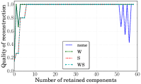
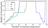
(a) RL60-2

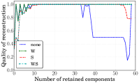
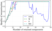
(b) RL60-10

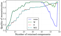
(c) WS60-2-.1

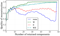
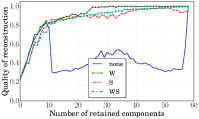
(d) WS60-2-.1

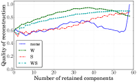
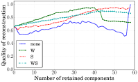
(e) SBM60-2

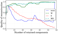
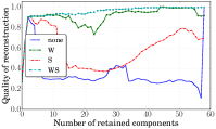
(f) SBM60-4

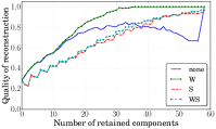
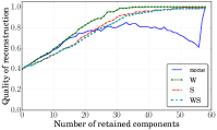
(g) ER60-.4

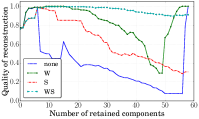
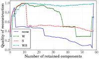
(h) BAR60

Figure 4: Results of the inverse transformation of a degraded collection of signals, obtained by retaining only a portion of the components. For each number of retained components, a quality of reconstruction is measured by comparing the obtained graph with the original one. Each sub-figure shows the results for one instance, whose name refers to those given in Figure 1. For each sub-figure, the left plot shows the results using thresholding based on the number of edges, while the right plot shows the results using the Adapted Otsu’s method. Four configurations of the inverse transformation are studied. none: no enhancement is performed; W: weighted computation of distances only with $\alpha=4$; S sequential update of the adjacency matrix only; WS both enhancements.

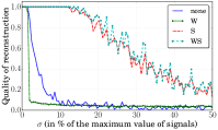
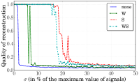
(a) RL60-2

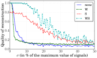
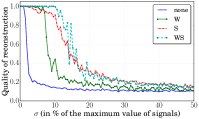
(b) RL60-10

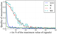
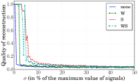
(c) WS60-2-.1

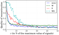
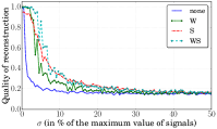
(d) WS60-2-.1

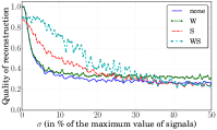
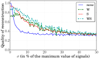
(e) SBM60-2

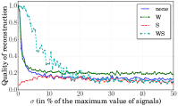
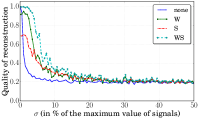
(f) SBM60-4

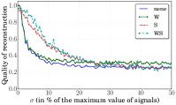
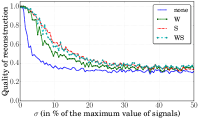
(g) ER60-.4

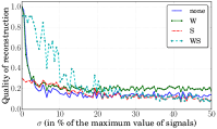
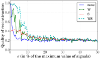
(h) BAR60

Figure 5: Results of the inverse transformation of a degraded collection of signals, obtained by adding Gaussian noise with mean $0$ and variance ranged from $0\%$ to $50\%$ of the maximal value of the signals. For each value of $\sigma$, a quality of reconstruction is measured by comparing the obtained graph with the original one. Each sub-figure shows the results for one instance, whose name refers to those given in Figure 1. For each sub-figure, the left plot shows the results using thresholding based on the number of edges, while the right plot shows the results using the Adapted Otsu’s method. Four configurations of the inverse transformation are studied. none: no enhancement is performed; W: weighted computation of distances only with $\alpha=4$; S sequential update of the adjacency matrix only; WS both enhancements.

Experimental setup

The performance of the robust inverse transformation using the proposed enhancements is evaluated in this section. A thorough evaluation is almost impossible: if the collection of signals is directly obtained using a transformation from graphs to signals as introduced in Section 2, then the inverse transformation is immediate and exact, and it does not require any sophisticated method. Conversely, if the collection of signals is not the representation of a graph, or if the signals are modified, there is no indication of the correct graph which is described at best by this collection. We propose nonetheless to assess the method by comparison of a graph with reconstructed versions after applying perturbations on the collection of signals.

Let us consider a graph $\mathcal{G}=(\mathcal{V},\mathcal{E})$, described by a collection of signals $\bm{X}$. The signals are perturbed to obtain a degraded collection of signals $\tilde{\bm{X}}$, whose inverse transformation gives a graph $\tilde{\mathcal{G}}=(\tilde{\mathcal{V}},\tilde{\mathcal{E}})$. $\mathcal{G}$ and $\tilde{\mathcal{G}}$ are compared by using an index of similarity, noted $Q(\mathcal{G},\tilde{\mathcal{G}})$, based on the Jaccard index [27] defined as $Q=\frac{|\mathcal{E}\cap\tilde{\mathcal{E}}|}{|\mathcal{E}\cup\tilde{\mathcal{E}}|}$, which compares the ratio of common edges between $\mathcal{G}$ and $\tilde{\mathcal{G}}$ over the total number of edges. $Q(\mathcal{G},\tilde{\mathcal{G}})$ is comprised between $0$, if all the edges are different, and $1$, if both graphs have the same edge set.

Two perturbations of the matrix $\bm{X}$ are studied. A first perturbation consists of removing low-energy components of a collection of signals: Starting from the first component, the components are successively added one by one in decreasing order of energy, until the collection is complete. The second perturbation consists in adding noise to the components: a Gaussian noise is added with mean $0$ and variance $\sigma$, ranged from $0\%$ to $50\%$ of the maximal value of the signals.

The inverse transformation is performed using the different enhancements of the method, in order to assess the contributions of each one. Four cases are then distinguished, according to the presence or absence of the weights in the computation of distances (with $\alpha=4$), and of the sequential update of the adjacency matrix: none (no enhancement), W (weighted computation of distances only), S (sequential update of the adjacency matrix only) and WS (both enhancements). Besides, the two methods of thresholding are tested separately in similar conditions. The experiments are performed on instances of graph models described in Section 2, in order to browse a wide variety of graph structures.

Results

Figures 4 and 5 show the results of the evaluation of the inverse transformation. Each sub-figure shows the results for one instance, whose name refers to those given in Figure 1. Since the Adapted Otsu’s method is not itself an enhancement but an alternative method to find a threshold of distances, the results have been divided for readability in two plots: For each sub-figure, the left plot shows the results without using thresholding based on the number of edges, while the right plot shows the results using the Adapted Otsu’s method.

Let us consider the case where the perturbation of the collection of signals $\bm{X}$ is obtained by retaining only a reduced number of components (Figure 4). We first focus on the left plots of each sub-figure, where the threshold is chosen by using the number of edges. Two configurations emerge from these results: W and WS. The gain in quality of reconstruction when using weighted distances is obvious, and reveals that this feature is the best contribution in the retrieval of the original graph. Adding S in combination with W does not affect significantly the score obtained with W alone, but without any improvement of the reconstruction, except for the instance (BAR60) in Figure 4h: In this case, only the combination of both enhancements gives good results. The comparison of the results in left and right plots shows that the choice of method of thresholding has a slight impact on the results when using the inverse transformation in configuration WS: the quality of reconstruction is quite similar in both cases. The Adapted Otsu’s method seems however less efficient when the number of retained components is low. An immediate explanation is that considering the number of edges of the original graph in the reconstruction gives undoubtedly a higher similarity between the reconstructed and the original graph than retaining only distances based on a discrimination, as it is performed in the Adapted Otsu’s method. Considering nonetheless that the latter method gives bad results when the number of retained components is low might be a cursory glance: with only few retained components, the actual graph described by $\tilde{\bm{X}}$ is likely to be quite far from the one described by $\bm{X}$. The Adapted Otsu’s method gives then a graph $\tilde{\mathcal{G}}$ which is not similar to $\mathcal{G}$, but which reflects the actual number of vertices.

Figure 5 shows the results for the second experiment, where the degraded collection of signals $\tilde{\bm{X}}$ is obtained by adding Gaussian noise to $\bm{X}$. Unexpectedly, the balance between the importance of W and S is the reverse: using enhancements S alone leads to better results than using W alone. The combination of both enhancements is nevertheless still the best method to reconstruct the graph from degraded collection of signals. The comparison between the two methods of thresholding is the same as in the previous case: Generally, results are a bit better when using the number of edges to select the threshold, especially when the perturbation is high.

To conclude this section about the inverse transformation, two contributions have been done to the method of inverse transformation to highly improve the quality of restoration from a degraded collection of signals. These results also show that not having the knowledge about the original graph does not penalize the inverse transformation, as it is possible to retrieve the correct number of edges from the signals. Besides, results give reasons to believe that the Adapted Otsu’s method leads to a graph which is closer to the actual graph represented by the perturbed collection of signals.

4 Analysis of signals representing graphs

The last section of this article is dedicated to the analysis of the collection of signals obtained after transformation from a graph. The aim of this part is to show how spectral analysis can be used to identify specific graph structures. As seen in Figure 1, signals present specific shapes which can be linked with the graph structure. Characterizing these shapes using spectral analysis enables us to associate frequency patterns with graph topology. Before that, we introduce the method of analysis by addressing an issue related to the indexation of signals.

4.1 Indexation of signals

So far, the importance of indexation of signals has been hidden since only relations, described by the Euclidean distances, have been of interest. Hence, the order in which we considered the vertices in the inverse transformation has no significance. However, this order is essential to study some spects of the signals, especially when using spectral analysis of the signals, as they are indexed by this vertex ordering. In Figure 1, the vertex ordering has been suitably defined to highlight specific shapes of signals: looking at the numbering of vertices in the graph representation shows that numbers closely follow the topology of the graph, in a “natural” order. Ordering randomly the vertices does not change the value assigned to each vertex, but would lead to abrupt variations in the representation of signals: Specific frequency properties, clearly observable in signals, will no longer be visible. Unfortunately, the suitable ordering is usually not available, especially when dealing with real-world graphs. To address this issue, we proposed in [25] to find a vertex ordering that reflects the topology of the underlying graph, based on the following assumption: if two vertices are close in the graph (by considering for instance the length of the shortest path between them), they have to be also close in the ordering. The method consists of the study of a related labeling problem, called cyclic bandwidth sum problem [28], defined in the more general framework of graph labeling problems [9]. These problems seek a mapping from vertices to integers, in such a way that an objective function, defined as the sum of the distances in the vertex ordering between all pairs of connected vertices, is minimized. The heuristic we proposed in [25] consists of a two-step algorithm. The first step performs local searches in order to find a collection of independent paths with respect to the local structure of the graph, while the second step determines the best way to arrange the paths such that the objective function of the cyclic bandwidth sum problem is minimized. Details of the algorithm and results about the consistency between the obtained vertex ordering and the topology of the graph are covered in [25].

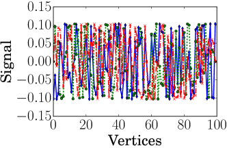
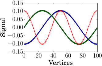
(a) 2-ring lattice

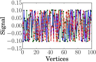
(b) Stochastic block model with 4 communities

Figure 6: Examples of transformation of two particular networks into signals, indexed by the vertices. The resulting collection of signals is indexed by the vertices. Three signals are displayed on each subplot as follows: Random ordering of vertices (Left), suitable ordering of vertices (Right).

Figure 6 shows two examples of transformation of two particular networks into signals. The resulting collection of signals is indexed by the vertices. Three signals are displayed on each subplot as follows: Random ordering of vertices (Left), suitable ordering of vertices (Right). It clearly shows that the ordering of the vertices has an influence on the spectral properties of the signals.

4.2 Connection between frequency patterns of signals and graph structures

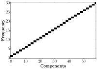
(a) RL60-2

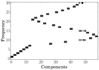
(b) RL60-10

(c) WS60-2-.1

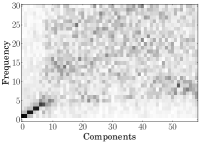
(d) WS60-10-.1

(e) SBM60-2

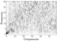
(f) SBM60-4

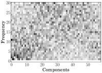
(g) ER60-.4

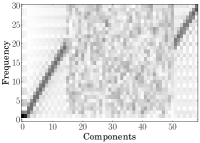
(h) BAR60

Figure 7: Frequency patterns obtained on instances of graphs defined in Section 2. Each pattern can be linked with the topology of the underlying graph. The color codes the intensities, from white to black.

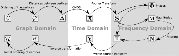
Figure 8: This diagram describes the process implemented to perform filtering of graphs using duality between graph and signals. The boxes describe the objects, while arrows represent the operations. The procedure is the following: From a graph $\mathcal{G}$, a collection of signals $\bm{X}$ is obtained by performing a good indexation of vertices and applying the CMDS method. A spectral analysis of the signals is then performed, and a matrix of magnitudes $\bm{M}$ is obtained. In the frequency domain, frequencies are truncated, leading to a matrix $\bm{N}$, which gives a new collection of signals $\bm{Y}$ by inverse Fourier transform. This process comes to apply a crude low-pass filtering on $\bm{X}$. A graph $\mathcal{H}$ is then computed from $\bm{Y}$, using the inverse transformation defined in Section 3. Each object belongs to a specific domain, either graph domain, time domain or frequency domain. Operations performs some processing of objects, such as filtering, as well as the mapping between the three domains.

Spectral analysis is performed using standard signal processing methods: Let a collection $\bm{X}$ of $K$ signals indexed by $n$ vertices, the spectrum $\bm{S}$ gives the complex Fourier coefficients whose elements are obtained by applying the Fourier transform on each of the $K$ components of $\bm{X}$: $s_{kf}=\mathcal{F}\bm{X}^{(k)}(f)$ estimated, for positive frequencies, on $F=\frac{n}{2}+1$ bins, $\mathcal{F}$ being the Fourier transform and $k\in\{1,\ldots,K\}$. From the spectrum $\bm{S}$, the magnitudes $\bm{M}$ of each frequency $f$ for each component read as: $M(k,f)=|s_{kf}|$. The matrix $\bm{M}$ is studied as a frequency-component map, exhibiting patterns in direct relation with the topology of the underlying graph. The phases of signals are stored in a matrix $\bm{\phi}$ to be used in the inverse Fourier transformation, when the collection of signals has to be retrieved from $\bm{M}$.

Fig. 7 shows the frequency patterns obtained for the graphs defined in Figure 1. Each graph highlights a specific frequency pattern, linked with its topology. Regular $k$-lattices display single-frequency components, whose order depends on the value of $k$: when $k$ is higher than $2$, the sorting of components is no longer consistent with the increasing order of frequencies, as described in Section 2.2. (Figures 7a and 7b). Adding noise to the graph also affects the patterns, as can be observed in Figures 7c and 7d. Graphs with communities are associated with highly-localized features: high-energy components, formed by plateaus corresponding to the communities, appear with high magnitudes for low frequencies in the first components (Figures 7e and 7f). These latter patterns are visible in the frequency-component map of the Barbell model in Figure 7h, denoting the combination of both structures in the graph. Finally, the magnitudes of random graphs, in Figure 7g, do not look like white noise spectra as the signals are re-indexed, and this removes the i.i.d. property and adds higher magnitudes on low frequencies for the first components than expected. Nonetheless, there is no specific pattern, which is consistent with the random structure of this graph.

4.3 Application to filtering of graphs

Throughout this article, we described tools to transform a graph into a collection of signals, analyze these signals to describe the graph, and finally transform back these signals into a graph, even if the collection of signals is not exactly the same. We propose here an application of these tools to perform filtering of graphs: in the same way as classical signals, graphs are often built from measurements, inducing noise, i.e., presence of undesirable edges or absence of existing edges. Figure 8 proposes a framework to use duality between graph and signals as a way to easily perform filtering on graph by filtering signals representing the graph.

The procedure is the following: From the matrix of magnitudes $\bm{M}$ obtained from a graph $\mathcal{G}$, a matrix $\bm{N}$ with the same shape is derived by retaining only the lowest frequencies. Using the matrix of phases $\bm{\phi}$, a degraded collection of signals $\bm{Y}$ is obtained by inverse Fourier transform. This process is tantamount to applying a crude low-pass filter on $\bm{X}$. A graph $\mathcal{H}$ is then computed from $\bm{Y}$, using the weighted distances with $\alpha=2$, the sequential update of the adjacency matrix and a thresholding using the Adapted Otsu’s method, as described in Section 3.

Figure 9 shows two examples of graph denoising, with on the left the adjacency matrix of the graph $\mathcal{G}$, and on the right the adjacency matrix of the graph $\mathcal{H}$, obtained after applying the process described in Figure 8. The first example is an instance of the Watts-Strogatz model (Figure 9a), corresponding to a noisy $k$-ring lattice (WS60-10-.1). The five lowest frequencies have been retained, and this leads to strengthening the diagonal, characterizing $k$-ring lattices. Besides, off-diagonal edges have been removed. The second example (Figure 9b) is an instance of the stochastic block model with communities (SBM60-2). This can be viewed in this case as two cliques whose random edges inside communities have been removed while random edges between communities have been added. After denoising, where the ten lowest frequencies of the matrix $\bm{M}$ have been retained, the missing edges inside communities are retrieved, while edges between them are removed: the communities are better-defined, appearing as actual cliques. These two examples highlight that denoising signals representing the graph is tantamount to denoising the graph itself.

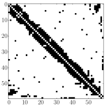
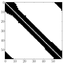
(a) WS60-10-.1

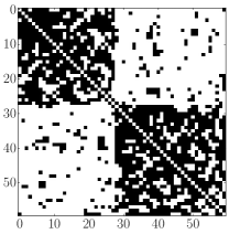
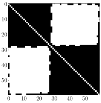
(b) SBM60-2

Figure 9: Illustrations of denoising of graphs, by applying the process described in Figure 8. The left plot gives the adjacency matrix of the graph $\mathcal{G}$, before filtering, while the right plot gives the adjacency matrix of the graph $\mathcal{H}$, after filtering. (a) The five lowest frequencies have been retained (b) The ten lowest frequencies have been retained.

5 Conclusion

In this article, we proposed a framework to study graphs in the classical domain of signals, enabling the analysis to take advantage of basic signal processing tools. From the method of transformation from graph to signals proposed by Shimada et al. [41], we discussed extensions to study the obtained signals and indirectly, the graph itself, using a robust inverse transformation. Denoising of graphs has been proposed to evaluate the method as a first potential application. The results we obtained suggest that the framework developed provides a connection between signal processing operations and modifications of graphs. This paves the road to new approach for the analysis of real-world networks, using more sophisticated signal processing tools, such as adaptive filtering.

Appendix A Upper bound for the parameter $w$

We propose here a rationale for the choice of $w$, based on the study of matrix eigenvalues: As mentioned in the work of Gower [18], $\bm{\Delta}$ is exactly retrieved from $\bm{X}$ if and only if $\bm{B}$ is positive definite:

$$\langle\bm{z},\bm{Bz}\rangle\geq 0\text{ for all vectors }\bm{z}\in\mathbb{R}^{n}$$ (3)

or equivalently, if and only if $\bm{\Delta}^{(2)}$ is conditionally negative definite:

$$\langle\bm{z},\bm{\Delta}^{(2)}\bm{z}\rangle\leq 0\quad{}\forall\bm{z}\in\mathbb{R}^{n}\text{ such that }\sum_{i=1}^{n}z_{i}=0$$ (4)

From the definition of $\bm{\Delta}$ in Eq. 1, we have:

$$\langle\bm{z},\bm{\Delta}^{(2)}\bm{z}\rangle =\langle\bm{z},\bm{A}\bm{z}\rangle$$ (5)

$$+w^{2}(\langle\bm{z},\bm{1}_{n}\bm{1}_{n}^{T}\bm{z}\rangle-\langle\bm{z},\bm{I}_{n}\bm{z}\rangle-\langle\bm{z},\bm{A}\bm{z}\rangle)$$

$$=\langle\bm{z},\bm{A}\bm{z}\rangle-w^{2}(\langle\bm{z},\bm{z}\rangle+\langle\bm{z},\bm{A}\bm{z}\rangle)$$

Two cases can be then distinguished:

1. If $\langle\bm{z},\bm{A}\bm{z}\rangle>-\langle\bm{z},\bm{z}\rangle$, then

   $$w^{2}\geq\frac{\langle\bm{z},\bm{A}\bm{z}\rangle}{\langle\bm{z},\bm{A}\bm{z}\rangle+\langle\bm{z},\bm{z}\rangle}$$ (6)

   which is hold as $w>1$.

2. If $\langle\bm{z},\bm{A}\bm{z}\rangle<-\langle\bm{z},\bm{z}\rangle$, then

   $$w^{2}\leq\frac{\langle\bm{z},\bm{A}\bm{z}\rangle}{\langle\bm{z},\bm{A}\bm{z}\rangle+\langle\bm{z},\bm{z}\rangle}$$ (7)

The upper bound depends on the adjacency matrix $\bm{A}$, i.e., on the structure of the graph. To have an idea of a suitable value of $w$, let us define $\bm{A}$ and $\bm{z}$ such that $\langle\bm{z},\bm{A}\bm{z}\rangle$ is minimal. $\bm{A}$ is defined as the adjacency matrix of a graph with $n$ vertices, with $n$ even, such that $a_{ij}=1$ if and only if $i$ and $j$ do not belong in the same subset among $\{1,\ldots,\frac{n}{2}\}$ and $\{\frac{n}{2}+1,\ldots,n\}$. $\bm{A}$ is then a $4$-block matrix, with the bottom-left block and the top-right block equal to $1$. As for $z$, it is equal to $-1$ for the first half of the vector and $1$ for the last half of the vector: $z=[-1,-1,\ldots,1,1]$. $\langle\bm{z},\bm{A}\bm{z}\rangle$ is then equal to $-\frac{n^{2}}{2}$, while $\langle\bm{z},\bm{z}\rangle=n$. Hence, we obtain an approximation for the upper bound of $w$: $w\leq\sqrt{\frac{n}{n-2}}$.

Appendix B Theoretical results for the $k$-ring lattices

A $k$-ring lattice is a graph where each vertex $i$ is connected to the vertices $\{i-\frac{k}{2},i-\frac{k}{2}+1,\ldots,i-1,i+1,\ldots,i+\frac{k}{2}-1,i+\frac{k}{2}\}$, for $k\in\{2,4,\ldots,n\}$. As Shimada et al. discussed in [41], it is immediate to find expected eigenvalues and eigenvectors in this case using circulant matrix theory [19]. We explicit additionally here the connection between the parameters $w$ and $k$ and the resulting signals. Any circulant matrix $\bm{C}$ has its eigenvalues $\bm{\lambda}$ given $\forall q\in\{0,n-1\}$ by $\lambda_{q}=\sum_{j=0}^{n-1}{c_{j}\zeta^{kj}}$ where $\bm{c}$ is the circulant vector of $\bm{C}$ and $\zeta=e^{\frac{2i\pi}{n}}$ is the $n$th root of the unity. As for eigenvectors, they are given $\forall q\in[0,n-1]$ by $\bm{v}_{q}=\sqrt{n}[1,\zeta^{q},\zeta^{2q},\ldots,\zeta^{(n-1)q}]$, corresponding to the columns of the Fourier matrix noted $\bm{F}^{(q)}$. These eigenvalues and eigenvectors appear as complex conjugate pairs, namely $\bar{\lambda}_{q}={\lambda}_{n-q}$ and $\bar{\bm{v}}_{q}=\bm{v}_{n-q}$ for $q\neq 0$. As we consider symmetric matrices, the eigenvalues are real and double ($\lambda_{q}={\lambda}_{n-q}$ for $q>0$) and the corresponding eigenvectors are the real and imaginary parts of $\bm{v}_{q}$, normalized by $\sqrt{2}$ to obtain an orthonormal matrix: $\bm{v}_{q}=\sqrt{2}\Re(\bm{F}^{(q)})=\sqrt{2}\cos(\frac{2\pi q}{n})$ and $\bm{v}_{n-q}=\sqrt{2}\Im(\bm{F}^{(q)})=\sqrt{2}\sin(\frac{2\pi q}{n})$, corresponding to harmonic oscillations. If $n$ is even, $\lambda_{\frac{n}{2}}$ is single and the corresponding eigenvector is not normalized by $\sqrt{2}$.

Starting from the circulant vector $\bm{\delta}$ with three values $0$, $1$ and $w$, the circulant vector $\bm{b}$ is defined by $b_{i}=-\frac{1}{2}[\delta_{i}^{2}-\frac{\alpha}{n}]$, with $\alpha=k+(n-1-k)w^{2}$. The vector $\bm{b}$ is then completely defined by three values: $\frac{\alpha}{2n}$ when $i=0$, $-\frac{\alpha}{2}(1-\frac{\alpha}{n})$ when $i\in\{1,\ldots,\frac{k}{2}\}\cup\{n-\frac{k}{2},\ldots,n-1\}$ and $-\frac{\alpha}{2}(w^{2}-\frac{\alpha}{n})$ when $i\in\{\frac{k}{2}+1,\ldots,n-\frac{k}{2}-1\}$. The computation of eigenvalues of $\bm{B}$ leads to $\lambda_{q}=\frac{\alpha}{2n}\sum_{j=0}^{n-1}{\zeta^{jq}}-\frac{1}{2}\left(\sum_{j=1}^{\frac{k}{2}}\zeta^{jq}+\sum_{j=n-\frac{k}{2}}^{n-1}\zeta^{jq}+w^{2}\sum_{j=\frac{k}{2}+1}^{n-\frac{k}{2}-1}\zeta^{jq}\right)$. From these eigenvalues, the obtained signals are similar to those obtained by standard methods of diagonalization of matrices, up to rotation, reflection and translation.

References

- [1] Ameya Agaskar and Yue M. Lu. A Spectral Graph Uncertainty Principle. IEEE Transactions on Information Theory, 59(7):4338–4356, July 2013.
- [2] B. Aguilar-San Juan and L. Guzmán-Vargas. Earthquake magnitude time series: scaling behavior of visibility networks. The European Physical Journal B, 86(11):454, 2013.
- [3] David Aldous and Jim Fill. Reversible Markov chains and random walks on graphs. Berkeley, 2002.
- [4] A. Anis, A. Gadde, and A. Ortega. Towards a sampling theorem for signals on arbitrary graphs. Acoustics, Speech and Signal Processing (ICASSP), 2014 IEEE International Conference on, pages 3864–3868, 4-9 May 2014.
- [5] Mikhail Belkin and Partha Niyogi. Laplacian Eigenmaps for Dimensionality Reduction and Data Representation. Neural Computation, 15(6):1373–1396, 2003.
- [6] Ingwer Borg and Patrick J. F Groenen. Modern Multidimensional Scaling. Springer Series in Statistics. Springer, 2005.
- [7] Andriana S. L. O. Campanharo, M. Irmak Sirer, R. Dean Malmgren, Fernando M. Ramos, and Luis A. N. Amaral. Duality between Time Series and Networks. PloS one, 6(8), 2011.
- [8] Siheng Chen, Rohan Varma, Aliaksei Sandryhaila, and Jelena Kovacevic. Discrete Signal Processing on Graphs: Sampling Theory. CoRR, abs/1503.05432, 2015.
- [9] Fan R.K. Chung. Labelings of graphs. In Selected topics in graph theory, volume 3, pages 151–168. 1988.
- [10] Fan RK Chung. Spectral graph theory, volume 92. American Mathematical Soc., 1997.
- [11] Yael Dekel, James R. Lee, and Nathan Linial. Eigenvectors of random graphs: Nodal Domains. Random Structures & Algorithms, 39(1):39–58, 2011.
- [12] Jonathan F. Donges, Jobst Heitzig, Reik V. Donner, and Jürgen Kurths. Analytical framework for recurrence network analysis of time series. Physical Review E, 85(4), 2012.
- [13] Reik V. Donner, Michael Small, Jonathan F. Donges, Norbert Marwan, Yong Zou, Ruoxi Xiang, and Jürgen Kurths. Recurrence-based time series analysis by means of complex network methods. International Journal of Bifurcation and Chaos, 21(04):1019–1046, 2011.
- [14] Richard Durrett. Random Graph Dynamics, volume 200. Cambridge University Press, 2007.
- [15] S. Fortunato. Community detection in graphs. Physics Reports, 486(3):75–174, 2010.
- [16] Akshay Gadde and Antonio Ortega. A Probabilistic Interpretation of Sampling Theory of Graph Signals. arXiv preprint arXiv:1503.06629, 2015.
- [17] Benjamin Girault, Paulo Gonçalves, Eric Fleury, and Arashpreet Singh Mor. Semi-Supervised Learning for Graph to Signal Mapping: a Graph Signal Wiener Filter Interpretation. In IEEE International Conference on Acoustics Speech and Signal Processing (ICASSP), pages 1115–1119, Florence, Italy, 2014.
- [18] John Clifford Gower. Properties of Euclidean and non-Euclidean distance matrices. Linear Algebra and its Applications, 67:81–97, 1985.
- [19] Robert M Gray. Toeplitz and circulant matrices: A review. Communications and Information Theory, 2(3):155–239, 2005.
- [20] David K. Hammond, Pierre Vandergheynst, and Rémi Gribonval. Wavelets on graphs via spectral graph theory. Applied and Computational Harmonic Analysis, 30(2):129–150, March 2011.
- [21] Ronan Hamon, Pierre Borgnat, Patrick Flandrin, and Céline Robardet. Networks as Signals, with an Application to Bike Sharing System. In Global Conference on Signal and Information Processing (GlobalSIP), 2013 IEEE, pages 611–614, Austin, Texas, USA, December 2013.
- [22] Ronan Hamon, Pierre Borgnat, Patrick Flandrin, and Céline Robardet. Tracking of a dynamic graph using a signal theory approach : application to the study of a bike sharing system. In ECCS’13, page 101, Barcelona, Spain, September 2013.
- [23] Ronan Hamon, Pierre Borgnat, Patrick Flandrin, and Céline Robardet. Transformation de graphes dynamiques en signaux non stationnaires. In Colloque GRETSI 2013, page 251, Brest, France, September 2013.
- [24] Ronan Hamon, Pierre Borgnat, Patrick Flandrin, and Céline Robardet. Nonnegative matrix factorization to find features in temporal networks. In IEEE International Conference on Acoustics Speech and Signal Processing (ICASSP), pages 1065–1069, Florence, Italy, 2014.
- [25] Ronan Hamon, Pierre Borgnat, Patrick Flandrin, and Céline Robardet. Discovering the structure of complex networks by minimizing cyclic bandwidth sum. Preprint arXiv:1410.6108, 2015.
- [26] Yuta Haraguchi, Yutaka Shimada, Tohru Ikeguchi, and Kazuyuki Aihara. Transformation from complex networks to time series using classical multidimensional scaling. In Artificial Neural Networks–ICANN 2009, pages 325–334. Springer, 2009.
- [27] Paul Jaccard. Etude comparative de la distribution florale dans une portion des Alpes et du Jura. Impr. Corbaz, 1901.
- [28] Hao Jianxiu. Cyclic bandwidth sum of graphs. Applied Mathematics-A Journal of Chinese Universities, 16(2):115–121, 2001.
- [29] Brian Karrer and M. E. J. Newman. Stochastic blockmodels and community structure in networks. Physical Review E, 83(1):016107, January 2011.
- [30] Antonio G. Marques, Santiago Segarra, Geert Leus, and Alejandro Ribeiro. Sampling of graph signals with successive local aggregations. arXiv preprint arXiv:1504.04687, 2015.
- [31] Marina Meila and Jianbo Shi. A Random Walks View of Spectral Segmentation. In 8th International Workshop on Artificial Intelligence and Statistics, 2001.
- [32] S.K. Narang and A. Ortega. Perfect Reconstruction Two-Channel Wavelet Filter Banks for Graph Structured Data. Signal Processing, IEEE Transactions on, 60(6):2786–2799, June 2012.
- [33] Mark Newman. Networks: An Introduction. Oxford University Press, Inc., New York, NY, USA, 2010.
- [34] H.Q. Nguyen and M.N. Do. Downsampling of Signals on Graphs Via Maximum Spanning Trees. Signal Processing, IEEE Transactions on, 63(1):182–191, January 2015.
- [35] Angel M. Nuñez, Lucas Lacasa, Jose Patricio Gomez, and Bartolo Luque. Visibility algorithms: A short review. INTECH Open Access Publisher, 2012.
- [36] Nobuyuki Otsu. A threshold selection method from gray-level histograms. Automatica, 11(285-296):23–27, 1975.
- [37] Bastien Pasdeloup, Réda Alami, Vincent Gripon, and Michael Rabbat. Toward An Uncertainty Principle For Weighted Graphs. arXiv preprint arXiv:1503.03291, 2015.
- [38] Fabrice Rossi. Visualization methods for metric studies. In Proceedings of the International Workshop on Webometrics, Informetrics and Scientometrics, pages 356–366, 2006.
- [39] Akie Sakiyama and Yuichi Tanaka. Oversampled Graph Laplacian Matrix for Graph Filter Banks. IEEE Transactions on Signal Processing, 62(24):6425–6437, December 2014.
- [40] A. Sandryhaila and J.M.F. Moura. Discrete Signal Processing on Graphs: Frequency Analysis. Signal Processing, IEEE Transactions on, 62(12):3042–3054, June 2014.
- [41] Yutaka Shimada, Tohru Ikeguchi, and Takaomi Shigehara. From Networks to Time Series. Phys. Rev. Lett., 109(15):158701, 2012.
- [42] Yutaka Shimada, Takayuki Kimura, and Tohru Ikeguchi. Analysis of chaotic dynamics using measures of the complex network theory. In Artificial Neural Networks-ICANN 2008, pages 61–70. Springer, 2008.
- [43] David I. Shuman, Sunil K. Narang, Pascal Frossard, Antonio Ortega, and Pierre Vandergheynst. The emerging field of signal processing on graphs: Extending high-dimensional data analysis to networks and other irregular domains. IEEE Signal Processing Magazine, 30(3):83–98, 2013.
- [44] David I Shuman, Benjamin Ricaud, and Pierre Vandergheynst. Vertex-frequency analysis on graphs. Applied and Computational Harmonic Analysis, February 2015.
- [45] J. B. Tenenbaum. A Global Geometric Framework for Nonlinear Dimensionality Reduction. Science, 290(5500):2319–2323, 2000.
- [46] Nicolas Tremblay and Pierre Borgnat. Graph Wavelets for Multiscale Community Mining. IEEE Transactions on Signal Processing, 62(20):5227–5239, 2014.
- [47] Mikhail Tsitsvero and Sergio Barbarossa. On the degrees of freedom of signals on graphs. Nice, France, 2015.
- [48] Mikhail Tsitsvero, Sergio Barbarossa, and Paolo Di Lorenzo. Signals on Graphs: Uncertainty Principle and Sampling. arXiv preprint arXiv:1507.08822, 2015.
- [49] Piet Van Mieghem. Graph spectra for complex networks. Cambridge University Press, 2011.
- [50] Duncan J. Watts and Steven H. Strogatz. Collective dynamics of ’small-world’ networks. Nature, 393(6684):440–442, 1998.
- [51] Tongfeng Weng, Yi Zhao, Michael Small, and Defeng (David) Huang. Time-series analysis of networks: Exploring the structure with random walks. Physical Review E, 90(2):022804, 2014.
- [52] J. Zhang and M. Small. Complex Network from Pseudoperiodic Time Series: Topology versus Dynamics. Physical Review Letters, 96(23):238701, 2006.