Gaps in the spectrum of a periodic quantum graph with periodically distributed $\delta^{\prime}$-type interactions

Abstract.

We consider a family of quantum graphs $\{(\Gamma,\mathcal{A}_{\varepsilon})\}_{\varepsilon>0}$, where $\Gamma$ is a $\mathbb{Z}^{n}$-periodic metric graph and the periodic Hamiltonian $\mathcal{A}_{\varepsilon}$ is defined by the operation $-\varepsilon^{-1}{\mathrm{d}^{2}\over\mathrm{d}x^{2}}$ on the edges of $\Gamma$ and either $\delta^{\prime}$-type conditions or the Kirchhoff conditions at its vertices. Here $\varepsilon>0$ is a small parameter. We show that the spectrum of $\mathcal{A}_{\varepsilon}$ has at least $m$ gaps as $\varepsilon\to 0$ ($m\in\mathbb{N}$ is a predefined number), moreover the location of these gaps can be nicely controlled via a suitable choice of the geometry of $\Gamma$ and of coupling constants involved in $\delta^{\prime}$-type conditions.

Keywords and phrases: periodic quantum graphs, $\delta^{\prime}$-type interactions, spectral gaps

1. Introduction

The name “quantum graph” is usually used for a pair $(\Gamma,\mathcal{A})$, where $\Gamma$ is a network-shaped structure of vertices connected by edges (“metric graph”) and $\mathcal{A}$ is a second order self-adjoint differential operator (“Hamiltonian”), which is determined by differential operations on the edges and certain interface conditions at the vertices. Quantum graphs arise naturally in mathematics, physics, chemistry and engineering as models of wave propagation in quasi-one-dimensional systems looking like a narrow neighbourhood of a graph. One can mention, in particular, quantum wires, photonic crystals, dynamical systems, scattering theory and many other applications. We refer to the recent monograph [3] containing a broad overview and comprehensive bibliography on this topic.

In many applications (for instance, to graphen and carbon nano-structures – cf. [17, 15]) periodic infinite graphs are studied. The metric graph $\Gamma$ is called periodic ($\mathbb{Z}^{n}$-periodic) if there is a group $G\simeq\mathbb{Z}^{n}$ acting isometrically, properly discontinuously and co-compactly on $\Gamma$ (cf. [3, Definition 4.1.1.]). Roughly speaking $\Gamma$ is glued from countably many copies of a certain compact graph $Y$ (“period cell”) and each $g\in G$ maps $Y$ to one of these copies.

In what follows in order to simplify the presentation (but without any loss of generality) we will assume that $\Gamma$ is embedded into $\mathbb{R}^{d}$ with $d=3$ as $n=1,2$ and $d=n$ as $n\geq 3$ and is invariant under translations through linearly independent vectors $e_{1},\dots,e_{n}$, i.e.

$$\Gamma=\Gamma+e_{j},\ j=1,\dots,n.$$ (1)

These vectors produce an action of $\mathbb{Z}^{n}$ on $\Gamma$. Such an embedding can be always realized.

An example of $\mathbb{Z}^{2}$-periodic graph is presented on Figure 1, its period cell is highlighted in bold lines.

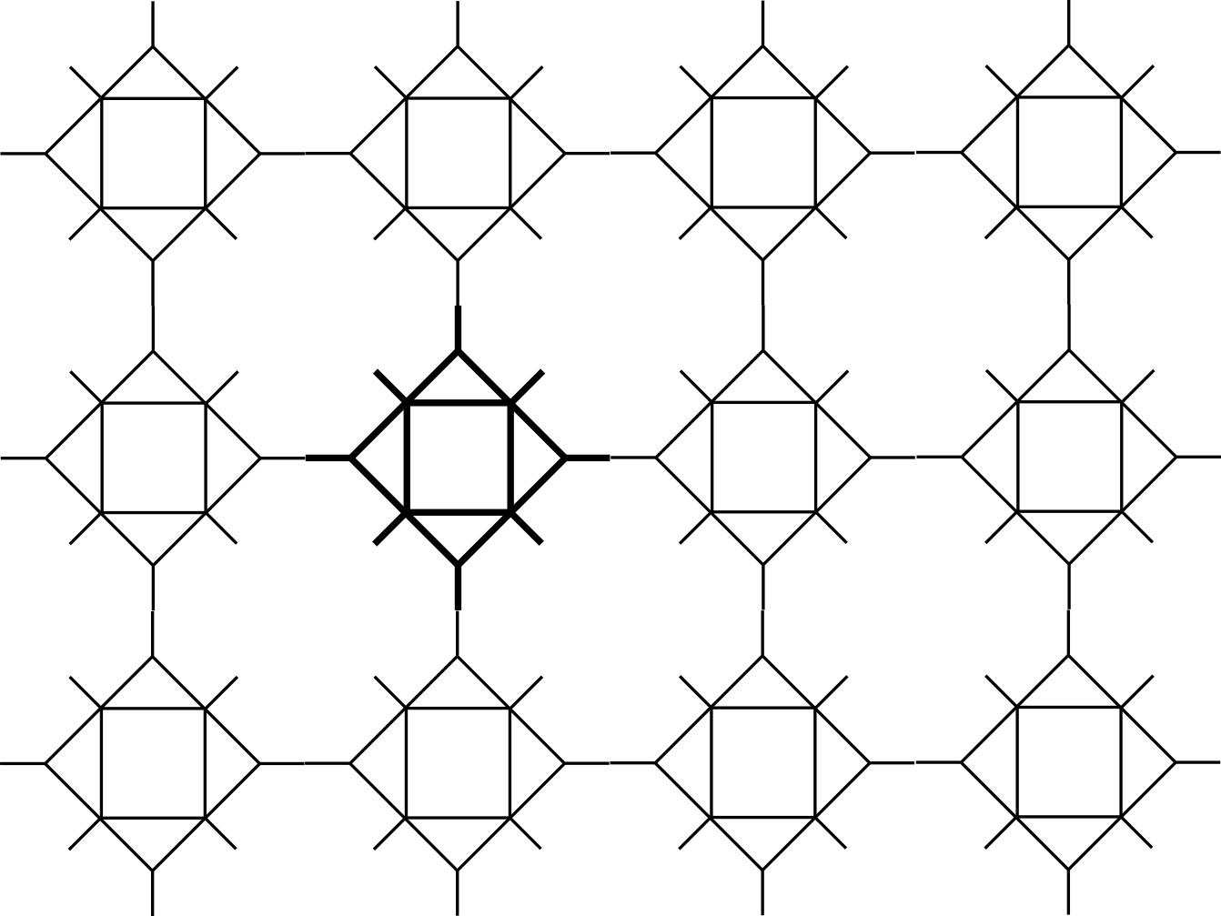
Figure 1. An example of $\mathbb{Z}^{2}$-periodic graph

The Hamiltonian $\mathcal{A}$ on a periodic metric graph $\Gamma$ is said to be periodic if it commutes with the action of $\mathbb{Z}^{n}$ on $\Gamma$. It is well-known (see, e.g., [3, Chapter 4]) that the spectrum of such operators has a band structure, i.e. it is a locally finite union of compact intervals called bands. In general the neighbouring bands may overlap. The bounded open interval $(\alpha,\beta)\subset\mathbb{R}$ is called a gap if it has an empty intersection with the spectrum, but its ends belong to it. In general the presence of gaps in the spectrum is not guaranteed – for example if $\Gamma$ is a rectangular lattice and $\mathcal{A}$ is defined by the operation $-{\mathrm{d}^{2}/\mathrm{d}x^{2}}$ on its edges and the Kirchhoff conditions at the vertices then the spectrum $\sigma(\mathcal{A})$ of the operator $\mathcal{A}$ has no gaps, namely $\sigma(\mathcal{A})=[0,\infty)$. Existence of spectral gaps is important because of various applications, for example in physics of photonic crystals.

There are several ways how to create quantum waveguides with spectral gaps. One of them is to use decorating graphs. Namely, given a fixed graph $\Gamma_{0}$ we “decorate” it attaching to each vertex of $\Gamma_{0}$ a copy of certain fixed graph $\Gamma_{1}$, the obtained graph we denote by $\Gamma$. Spectral properties of such graphs were studied in [21], where operators defined on functions on vertices were considered (“discrete graphs”). The case of quantum graphs was studied in [16] and it was proved that gaps open up in the spectrum of the operator defined by the operation $-{\mathrm{d}^{2}/\mathrm{d}x^{2}}$ on the edges of $\Gamma$ and the Kirchhoff conditions at the vertices (other conditions are also allowed); these gaps are located around eigenvalues of a certain Hamiltonian on $\Gamma_{1}$.

Also one can use “spider decoration” procedure: in each vertex we disconnect the edges emerging from it and then connect their loose endpoints by a certain additional graph (“spider”). Such decorating procedure was probably used for the first time in [2, 6], more results on gap opening one can find in [19].

Another way to create gaps, instead of to perturb a graph geometry, is to substitute the Kirchhoff conditions at the vertices by more “advanced” ones. For example, let $\Gamma$ be a rectangular lattice and $\mathcal{A}$ be defined by the operation $-{\mathrm{d}^{2}/\mathrm{d}x^{2}}$ on its edges and $\delta$ conditions at the vertices, i.e. the functions from $\mathrm{dom}(\mathcal{A})$ are continuous at all vertices and the sum of their derivatives is proportional to the value of a function at the vertex with a coupling constant $\alpha\in\mathbb{R}$ (the case $\alpha=0$ corresponds to the Kirchhoff conditions). Then (cf. [6, 7]) the spectrum $\sigma(\mathcal{A})$ has infinitely many gaps provided $\alpha\not=0$ and the lattice-spacing ratio satisfies some additional mild assumptions.

The goal of the current paper is to study spectral properties of some specific class of periodic quantum graphs. The main peculiarity of these graphs is that their spectral gaps can be nicely controlled via a suitable choice of the graph geometry and of coupling constants involved in interface conditions at its vertices.

Figure 2. The example of the graph $\Gamma$. Here $m=2$.

In particular, for a given $m\in\mathbb{N}$ we construct a family $\left\{(\Gamma,\mathcal{A}_{\varepsilon})\right\}_{{\varepsilon}>0}$ of periodic quantum graphs having at least $m$ gaps as ${\varepsilon}$ is small enough and moreover the first $m$ gaps converge to predefined intervals as ${\varepsilon}\to 0$. The graph $\Gamma$ is constructed as follows. We take an arbitrary $\mathbb{Z}^{n}$-periodic graph $\Gamma_{0}$ with vectors $e_{1},\dots,e_{n}$ producing an action of $\mathbb{Z}^{n}$ on it and attach to $\Gamma_{0}$ a family of compact graphs $Y_{ij}$, $i=(i_{1},\dots,i_{n})\in\mathbb{Z}^{n}$, $j=1,\dots,m$ satisfying $Y_{0j}+\sum\limits_{k=1}^{n}i_{k}e_{k}=Y_{ij}$. We denote by $\Gamma$ the obtained graph (an example is presented on Figure 2) and consider on it the Hamiltonian $\mathcal{A}_{\varepsilon}$ defined by the operation

$$-\displaystyle{{\varepsilon}^{-1}}{\mathrm{d}^{2}\over\mathrm{d}x^{2}}$$

on its edges and the Kirchhoff conditions in all its vertices except the points of attachment of $Y_{ij}$ to $\Gamma_{0}$ – in these points we pose $\delta^{\prime}$-type conditions (in the case of vertex with two outgoing edges they coincide with the usual $\delta^{\prime}$ conditions at a point on the line – cf. [1, Sec. I.4]). The required structure for the spectrum of $\mathcal{A}_{\varepsilon}$ is achieved via a suitable choice of coupling constants involved in $\delta^{\prime}$-type conditions and of ”sizes” of attached graphs.

2. Setting of the problem and main result

2.1. Graph $\Gamma$

Let

$$\Gamma=(\mathcal{V},\mathcal{E},\gamma,l)$$

be a connected $\mathbb{Z}^{n}$-periodic metric graph. Here

• by $\mathcal{V}$ we denote the set of its vertices,

• by $\mathcal{E}$ we denote the set of its edges,

• the map $\gamma:\mathcal{E}\to\mathcal{V}\times\mathcal{V}$ assigns to each edge $e$ its initial and terminal points (we denote them $\gamma^{-}(e)$ and $\gamma^{+}(e)$, correspondingly),

• the function $l:\mathcal{E}\to(0,\infty)$ assigns to the edge $e$ its length $l(e)$.

We suppose that the degree of each vertex (i.e., the number of edges emanating from it) is finite. In order to simplify the presentation we assume that $\Gamma$ is embedded into $\mathbb{R}^{d}$, where $d=3$ as $n=1,2$ and $d=n$ as $n\geq 3$.

On each edge $e\in\mathcal{E}$ we introduce the local coordinate $x_{e}\in[0,l(e)]$ in such a way that $x_{e}=0$ corresponds to $\gamma^{-}(e)$ and $x_{e}=l(e)$ corresponds to $\gamma^{+}(e)$. One can assume that $\Gamma$ has no loops (i.e. there is no edge $e$ with $\gamma^{+}(e)=\gamma^{-}(e)$), otherwise one can break them into pieces by introducing a new intermediate vertex. For $v\in\mathcal{V}$ we denote

$$\mathcal{E}(v)=\left\{\text{the set of edges outgoing from }v\right\}.$$

In a natural way the function $l$ gives rise to a metric on $\Gamma$. In what follows by $\overset{\circ}{Z}$ (or $\mathrm{int}Z$), $\overline{Z}$, $\partial Z$ we denote, correspondingly, the interior, the closure, the boundary of a subset $Z\subset\Gamma$ with respect to this metric. In particular, $\partial\Gamma$ consists of the vertices of $\Gamma$ of degree $1$.

The $\mathbb{Z}^{n}$-periodicity of $\Gamma$ means that there are linearly independent vectors $e_{1},\dots,e_{n}$ satisfying (1). By $Y$ we denote a period cell of $\Gamma$, that is a compact subset of $\Gamma$ satisfying

$$\overset{\circ}{Y}\cap\left(\overset{\circ}{Y}+\sum\limits_{k=1}^{n}i_{k}e_{k}\right)=\varnothing\text{ for an arbitrary }i=(i_{1},\dots,i_{n})\in\mathbb{Z}^{n}\setminus\{0\},$$

$$\Gamma=\bigcup\limits_{i\in\mathbb{Z}^{n}}\left(Y+\sum\limits_{k=1}^{n}i_{k}e_{k}\right).$$

We notice that period cell is not uniquely defined.

The period cell $Y$ can be always chosen in such a way that $\partial Y$ does not contain any vertex $v\in\mathcal{V}\setminus\partial\Gamma$ (see Figure 1). Under such a choice of the period cell the boundary $\partial Y$ of $Y$ consists of two disjoint parts $\partial_{\mathrm{int}}Y$ and $\partial_{\mathrm{ext}}Y$, where

• $\partial_{\mathrm{int}}Y$ consists of vertices of $\Gamma$ of degree $1$ belonging to $Y$,

• $\partial_{\mathrm{ext}}Y$ consists of vertices of $Y$ of degree $1$ lying in the interiors of certain edges of $\Gamma$.

An example of $\mathbb{Z}^{2}$-periodic graph is presented on Figure 1. Its period cell $Y$ is presented in more details on Figure 3 and one has

$$\partial_{\mathrm{int}}Y=\left\{v_{13},v_{14},v_{15},v_{16},\right\},\quad\partial_{\mathrm{ext}}Y=\left\{v_{1},v_{5},v_{8},v_{11}\right\}.$$

Figure 3. Period cell of the graph from Figure 1

Additionally, we suppose that $Y$ can be expressed as a union of $m+1$ compact subsets,

$$Y=\bigcup\limits_{j=0}^{m}Y_{j},\ m\in\mathbb{N},$$ (2)

satisfying the following conditions:

$$\begin{array}[]{ll}\text{(i)\quad}&\overset{\circ}{Y_{j}}\not=\varnothing,\\ \vspace{1pt}\text{(ii)\quad}&Y_{j}\text{ are connected,}\\ \vspace{1pt}\text{(iii)\quad}&\textrm{int}(Y_{j}\cap Y_{k})=\varnothing\text{ provided }j\not=k,\\ &\text{i.e. $Y_{j}$ and $Y_{k}$ may have only common vertices, not edges},\\ \vspace{1pt}\text{(iv)\quad}&\partial_{\mathrm{ext}}Y\subset\partial Y_{0},\\ \vspace{1pt}\text{(v)\quad}&\text{the sets }\mathcal{V}_{j}:=\partial Y_{0}\cap\partial Y_{j},\ j=1,\dots,m\text{ are nonempty},\\ \vspace{1pt}\text{(vi)\quad}&\text{if }j,k\not=0\text{ and }j\not=k\text{ then either }\partial Y_{j}\cap\partial Y_{k}=\varnothing\text{ or }\partial Y_{j}\cap\partial Y_{k}\subset\partial Y_{0}.\end{array}$$ (10)

Remark 2.1.

In fact, decomposition (2) satisfying (10) is always possible for an arbitrary graph $\Gamma\ncong\mathbb{R}$ under a suitable choice of a period cell. Let us formulate this statement more accurately. At first we notice that for an arbitrary $s\in\mathbb{N}$ condition (1) holds with $e^{s}_{j}:=se_{j}$ instead of $e_{j}$, $j=1,\dots,n$ (i.e., $\Gamma$ is periodic with respect to the period cell $Y^{s}:=sY$). It is easy to see that if $\Gamma\ncong\mathbb{R}$ then $Y^{s}$ contains $m$ edges $\tilde{e}_{1},\dots,\tilde{e}_{m}$ satisfying

$$\tilde{e}_{i}\cap\tilde{e}_{j}=\varnothing\text{ as }i\not=j,\quad Y_{0}:=\overline{Y^{s}\setminus\bigcup\limits_{j=1}^{n}{\tilde{e}_{j}}}\text{ is a connected set},\quad\overset{\circ}{Y_{0}}\not=\varnothing,\quad\partial_{\mathrm{ext}}Y^{s}\subset\partial Y_{0}$$

provided $s$ is large enough. We set $Y_{j}:=\tilde{e}_{j}$, $j=1,\dots,m$. Obviously, $Y^{s}=\bigcup\limits_{j=0}^{m}Y_{j}$ and conditions (10) hold true.

It is easy to see that $\bigcup\limits_{j=1}^{m}\mathcal{V}_{j}\subset\overset{\circ}{Y}$. One can assume that the set $\bigcup\limits_{j=1}^{m}\mathcal{V}_{j}$ belongs to $\mathcal{V}$, otherwise if some of its points belongs to the interior of an edge then we can add it to $\mathcal{V}$ (as a vertex with two outgoing edges). Finally, for $i=(i_{1},\dots,i_{n})\in\mathbb{Z}^{n}$, $j\in\{1,\dots,m\}$ we set

$$\mathcal{V}_{ij}=\mathcal{V}_{j}+\sum\limits_{k=1}^{n}i_{k}e_{k}.$$

The points belonging to $\mathcal{V}_{ij}$ will support our $\delta^{\prime}$-type conditions.

Also we will use the notation

$$Y_{ij}:=Y_{j}+\sum\limits_{k=1}^{n}i_{k}e_{k},\quad i=(i_{1},\dots,i_{n})\in\mathbb{Z}^{n},\ j\in\{1,\dots,m\}.$$

Let us come back to the example depicted on Figure 3. There are several possibilities to decompose the period cell in a way described above. For example, one has $Y=Y_{0}\cup Y_{1}$,

• $Y_{0}$ consists of the edges $e_{1},e_{2},e_{4},e_{5},e_{6},e_{8},e_{9},e_{10},e_{12},e_{13},e_{14},e_{16}$ (solid lines),

• $Y_{1}$ consists of the edges $e_{3},e_{7},e_{11},e_{15},e_{17},e_{18},e_{19},e_{20}$ (dash-dotted lines).

The set $\mathcal{V}_{1}$ consists of the vertices $v_{3},v_{6},v_{9},v_{12}$.

One can also decompose $Y$ in a more “advanced” way, for example as a union of six sets:

• $Y_{0}$ consists of the edges $e_{1},e_{2},e_{4},e_{5},e_{6},e_{8},e_{9},e_{10},e_{12},e_{13},e_{14},e_{16}$,

• $Y_{1}$ consists of the edges $e_{17},e_{18},e_{19},e_{20}$,

• $Y_{2}$ consists of the edge $e_{3}$,

• $Y_{3}$ consists of the edge $e_{7}$,

• $Y_{4}$ consists of the edge $e_{11}$,

• $Y_{5}$ consists of the edge $e_{15}$.

Then $\mathcal{V}_{1}=\{v_{3},v_{6},v_{9},v_{12}\}$, $\mathcal{V}_{2}=\{v_{3}\},\ \mathcal{V}_{3}=\{v_{6}\},\ \mathcal{V}_{4}=\{v_{9}\},\ \mathcal{V}_{5}=\{v_{12}\}.$

2.2. Hamiltonian $\mathcal{A}_{\varepsilon}$

In what follows if $u:\Gamma\to\mathbb{C}$ and $e\in\mathcal{E}$ then by $u_{e}$ we denote the restriction of $u$ onto $\overset{\circ}{e}$. Via a local coordinate $x_{e}$ we identify $u_{e}$ with a function on $(0,l(e))$.

We introduce several functional spaces on $\Gamma$. The space $L_{2}(\Gamma)$ consists of functions that are measurable and square integrable on each edge and such that

$$\|u\|^{2}_{L_{2}(\Gamma)}:=\sum\limits_{e\in\mathcal{E}}\|u_{e}\|^{2}_{L_{2}\left(0,l(e)\right)}=\sum\limits_{e\in\mathcal{E}}\int\limits_{0}^{l(e)}|u_{e}(x_{e})|^{2}\mathrm{d}x_{e}<\infty.$$

The space $\widetilde{H}^{k}(\Gamma)$, $k\in\mathbb{N}$ consists of functions on $\Gamma$ belonging to the Sobolev space $H^{k}(e)$ on each edge $e\in\mathcal{E}$ and satisfying

$$\|u\|^{2}_{\widetilde{H}^{k}(\Gamma)}:=\sum\limits_{e\in\mathcal{E}}\|u_{e}\|^{2}_{H^{k}\left(0,l(e)\right)}=\sum\limits_{e\in\mathcal{E}}\sum\limits_{l=0}^{k}\int\limits_{0}^{l(e)}\left|\mathrm{d}^{l}u_{e}(x_{e})\over\mathrm{d}x_{e}^{l}\right|^{2}\mathrm{d}x_{e}<\infty.$$

Finally, the set $\mathcal{H}(\Gamma)$ consists of functions $u\in\widetilde{H}^{1}(\Gamma)$ satisfying the following conditions at vertices of $\Gamma$:

• if $v\in\mathcal{V}\setminus\left(\bigcup\limits_{i\in\mathbb{Z}^{n}}\bigcup\limits_{j=1}^{m}\mathcal{V}_{ij}\right)$ then $u$ is continuous at $v$, i.e. the limiting value of $u(x)$ when $x$ approaches $v$ along $e\in\mathcal{E}(v)$ is independent of $e$. We denote this value by $u(v)$;

• if $v\in\mathcal{V}_{ij}$ for some $i=(i_{1},\dots,i_{n})\in\mathbb{Z}^{n}$, $j\in\{1,\dots,m\}$ then

  • the limiting value of $u(x)$ when $x$ approaches $v$ along $e\in\mathcal{E}(v)\cap Y_{i0}$ is independent of $e$. We denote this value by $u_{0}(v)$;

  • the limiting value of $u(x)$ when $x$ approaches $v$ along $e\in\mathcal{E}(v)\cap Y_{ij}$ is independent of $e$. We denote this value by $u_{j}(v)$.

Now, we describe the family of operators $\mathcal{A}_{\varepsilon}$, which will the main object of our interest in this paper. In $L_{2}(\Gamma)$ we introduce the sesquilinear form $a_{\varepsilon}$,

$$\mathrm{dom}(a_{\varepsilon})=\mathcal{H}(\Gamma),$$

$$a_{\varepsilon}[u,w]={{\varepsilon}^{-1}}\sum\limits_{e\in\mathcal{E}}\int\limits_{0}^{l(e)}{\mathrm{d}u_{e}\over\mathrm{d}x_{e}}\overline{\mathrm{d}w_{e}\over\mathrm{d}x_{e}}\mathrm{d}x_{e}+\sum\limits_{i\in\mathbb{Z}^{n}}\sum\limits_{j=1}^{m}\sum\limits_{v\in\mathcal{V}_{ij}}q_{j}\left(u_{0}(v)-u_{j}(v)\right)\overline{\left(w_{0}(v)-w_{j}(v)\right)},$$ (11)

where $q_{j}$ are positive constants. The definition of $a_{\varepsilon}[u,w]$ makes sense: the second term in the right-hand-side of (11) (we denote it $\tilde{a}[u,w]$) is finite, namely one has the estimate

$$|\tilde{a}[u,w]|^{2}\leq C\|u\|^{2}_{\widetilde{H}^{1}(\Gamma)}\|w\|^{2}_{\widetilde{H}^{1}(\Gamma)}$$

following from the standard trace inequality

$$|u(l)|^{2}\leq 2\left({l}^{-1}\|u\|^{2}_{L_{2}(0,l)}+l\|u^{\prime}\|^{2}_{L_{2}(0,l)}\right),\ \forall u\in H^{1}(0,l).$$

Furthermore, it is straightforward to check that the form $a_{\varepsilon}[u,v]$ is symmetric, densely defined, closed and positive. Then (see, e.g., [20, Theorem VIII.15]) there exists the unique self-adjoint and positive operator $\mathcal{A}_{\varepsilon}$ associated with the form $a_{\varepsilon}$, i.e.

$$(\mathcal{A}_{\varepsilon}u,v)_{L_{2}(\Gamma)}=a_{\varepsilon}[u,v],\quad\forall u\in\mathrm{dom}(\mathcal{A}_{\varepsilon}),\ \forall v\in\mathrm{dom}(a_{\varepsilon}).$$

The definitional domain of the operator $\mathcal{A}_{\varepsilon}$ consists of functions $u\in\mathcal{H}(\Gamma)$ belonging to $\widetilde{H}^{2}(\Gamma)$ and satisfying the following conditions at the vertices (additionally to the conditions needed to be in $\mathcal{H}(\Gamma)$):

• if $v\in\mathcal{V}\setminus\bigcup\limits_{i\in\mathbb{Z}^{n}}\bigcup\limits_{j=1}^{m}\{v_{ij}\}$ then

  $$\sum\limits_{e\in\mathcal{E}(v)}\left.{\mathrm{d}u_{e}\over\mathrm{d}\mathbf{x}_{e}}\right|_{\mathbf{x}_{e}=0}=0\qquad(\text{Kirchhoff conditions}),$$

  where

  $$\mathbf{x}_{e}=\begin{cases}x_{e},&\text{if }v=\gamma^{-}(e),\\ \mathbf{x}_{e}=l(e)-x_{e},&\text{if }v=\gamma^{+}(e)\end{cases}$$

  (i.e. $\mathbf{x}_{e}$ is a natural coordinate on $e\in\mathcal{E}(v)$ such that $\mathbf{x}_{e}=0$ at $v$);

• if $v\in\mathcal{V}_{ij}$, $i\in\mathbb{Z}^{n}$, $j\in\{1,\dots,m\}$ one has the following conditions at $v$:

  $$\begin{array}[]{c}\displaystyle-{\varepsilon}^{-1}\sum\limits_{e\in\mathcal{E}(v)\cap Y_{i0}}\left.{\mathrm{d}u_{e}\over\mathrm{d}\mathbf{x}_{e}}\right|_{\mathbf{x}_{e}=0}+q_{j}(u_{0}(v)-u_{j}(v))=0,\\ \displaystyle-{\varepsilon}^{-1}\sum\limits_{e\in\mathcal{E}(v)\cap Y_{ij}}\left.{\mathrm{d}u_{e}\over\mathrm{d}\mathbf{x}_{e}}\right|_{\mathbf{x}_{e}=0}+q_{j}(u_{j}(v)-u_{0}(v))=0.\end{array}\qquad\text{($\delta^{\prime}$-type conditions)}$$ (14)

The operator $\mathcal{A}_{\varepsilon}$ acts as follows:

$$\left(\mathcal{A}_{\varepsilon}u\right)_{e}=-{\varepsilon}^{-1}{\mathrm{d}^{2}u_{\varepsilon}\over\mathrm{d}x^{2}_{e}},\ e\in\mathcal{E}.$$

Remark 2.2.

Suppose that $v\in\mathcal{V}_{ij}$ (for some $i\in\mathbb{Z}^{n}$, $j\in\{1,\dots,m\}$) has two outgoing edges, $e\in\mathcal{E}(v)\cap Y_{ij}$ and $\tilde{e}\in\mathcal{E}(v)\cap Y_{i0}$. Then, evidently, conditions (14) are equivalent to

$$\left.{\mathrm{d}u_{e}\over\mathrm{d}\mathbf{x}_{e}}\right|_{\mathbf{x}_{e}=0}+\left.{\mathrm{d}u_{\tilde{e}}\over\mathrm{d}\mathbf{x}_{\tilde{e}}}\right|_{\mathbf{x}_{\tilde{e}}=0}=0,\quad\kappa\displaystyle\left.{\mathrm{d}u_{e}\over\mathrm{d}\mathbf{x}_{e}}\right|_{\mathbf{x}_{e}=0}=\left(\left.u_{e}\right|_{\mathbf{x}_{e}=0}-\left.u_{\tilde{e}}\right|_{\mathbf{x}_{\tilde{e}}=0}\right),\ \kappa=(q_{j}{\varepsilon})^{-1},$$

(recall that $\mathbf{x}_{e}\in[0,l(e)]$ and $\mathbf{x}_{\tilde{e}}\in[0,l(\tilde{e})]$ are the natural coordinates on $e$ and $\tilde{e}$, correspondingly, such that $\mathbf{x}_{e}=\mathbf{x}_{\tilde{e}}=0$ at $v$). Thus we obtain the usual $\delta^{\prime}$ conditions at a point on the line [1, Sec. I.4] that explains why we use the term “$\delta^{\prime}$-type conditions” for (14). Various analogues of $\delta^{\prime}$ conditions for graphs are discussed in [7].

Remark 2.3.

The name “$\delta^{\prime}$-conditions” is misleading because such Hamiltonians cannot be obtained using families of scaled zero-mean potentials (cf. [22]). However one can approximate them by a triple of $\delta$ potentials and then by regular $\delta$-like ones following an idea put forward in [4] and then made mathematically rigorous in [9]. The problem of approximating all singular vertex couplings (in particular, $\delta^{\prime}$-type ones) in a quantum graph is solved in [5].

2.3. The main result

Before to formulate the result let us introduce several notations.

We denote

• by $l_{j}$, $j=0,\dots,m$ the total length of all edges belonging to $Y_{j}$,

• by $N_{j}$, $j=1,\dots,m$ we denote the number of points belonging to the set $\mathcal{V}_{j}$.

Then for $j=1,\dots,m$ we set:

$$a_{j}:={N_{j}q_{j}\over l_{j}}.$$ (15)

It is assumed that the numbers $a_{j}$ are pairwise non-equivalent. We renumber them in the ascending order, that is

$$a_{j}<a_{j+1},\ \forall j=1,\dots,m-1.$$ (16)

Finally, we consider the following equation (with unknown $\lambda\in\mathbb{C}$):

$$\mathcal{F}(\lambda):=1+\sum\limits_{i=1}^{m}{a_{i}l_{i}\over l_{0}(a_{i}-\lambda)}=0.$$ (17)

It is straightforward to show that if (16) holds then equation (17) has exactly $m$ roots, they are real and interlace with $a_{j}$. We denote them by $b_{j}$, $j=1,\dots,m$ supposing that they are renumbered in the ascending order, i.e.

$$a_{j}<b_{j}<a_{j+1},\ j={1,\dots,m-1},\quad a_{m}<b_{m}<\infty.$$ (18)

We are now in position to formulate the first main result of this work.

Theorem 2.1.

Let $L>0$ be an arbitrary number. Then the spectrum of the operator $\mathcal{A}_{\varepsilon}$ in $[0,L]$ has the following structure for ${\varepsilon}$ small enough:

$$\sigma(\mathcal{A}_{\varepsilon})\cap[0,L]=[0,L]\setminus\bigcup\limits_{j=1}^{m}\big{(}a_{j}({\varepsilon}),b_{j}({\varepsilon})\big{)},$$ (19)

where the endpoints of the intervals $\big{(}a_{j}({\varepsilon}),b_{j}({\varepsilon})\big{)}$ satisfy the relations

$$\lim\limits_{{\varepsilon}\to 0}a_{j}({\varepsilon})=a_{j},\quad\lim\limits_{{\varepsilon}\to 0}b_{j}({\varepsilon})=b_{j},\ j=1,\dots,m.$$ (20)

In the last section we will present our second result (Theorem 4.1): we will show that under a suitable choice of the graph $\Gamma$ and the coupling constants $q_{j}$ the limit intervals $(a_{j},b_{j})$ coincide with predefined ones.

Theorem 2.1 will be proven in the next section. We postpone the outline of the proof to the end of Subsection 3.1 because we need to introduce first some more notations.

3. Proof of Theorem 2.1

3.1. Preliminaries

The Floquet-Bloch theory establishes a relationship between the spectrum of $\mathcal{A}_{\varepsilon}$ and the spectra of appropriate operators on $Y$. Namely, let

$$\theta\in\mathbb{T}^{n}=\{\theta=(\theta_{1},\dots,\theta_{n})\in\mathbb{C}^{n},\ |\theta_{k}|=1\text{ for all }k=1,\dots,n\}.$$

We denote by $\mathcal{H}^{\theta}(\Gamma)$ the set of functions $u:\Gamma\to\mathbb{C}$ satisfying

• $\forall e\in\mathcal{E}$: $u_{e}\in H^{1}(e)$,

• $u$ is continuous at all vertices belonging to $\mathcal{V}\setminus\left(\bigcup\limits_{i\in\mathbb{Z}^{n}}\bigcup\limits_{j=1}^{m}\mathcal{V}_{ij}\right)$,

• at the vertices belonging to $\bigcup\limits_{i\in\mathbb{Z}^{n}}\bigcup\limits_{j=1}^{m}\mathcal{V}_{ij}$ $u$ satisfies the same conditions as functions from $\mathcal{H}(\Gamma)$,

• $u$ is $\theta$-periodic, that is

  $$\forall x\in\Gamma:u(x+e_{k})=\theta_{k}u(x),\ k=1,\dots,n$$

  (if $\theta=(1,1,\dots,1)$ (respectively, $\theta=-(1,1,\dots,1)$) one has periodic (respectively, antiperiodic) conditions).

Then we introduce the sesquilinear form $a_{\varepsilon}^{\theta}$ defined as follows (below the notation $\mathcal{E}(Y)$ stays for the set of edges of $Y$):

$$\mathrm{dom}(a_{\varepsilon}^{\theta})=\left\{u=v|_{Y},\ v\in\mathcal{H}^{\theta}(\Gamma)\right\},$$

$$a^{\theta}_{\varepsilon}[u,w]={\varepsilon}^{-1}\sum\limits_{e\in\mathcal{E}(Y)}\int\limits_{0}^{l(e)}{\mathrm{d}u_{e}\over\mathrm{d}x_{e}}\overline{\mathrm{d}w_{e}\over\mathrm{d}x_{e}}\mathrm{d}x_{e}+\sum\limits_{j=1}^{m}\sum\limits_{v\in\mathcal{V}_{j}}q_{j}\left(u_{0}(v)-u_{j}(v)\right)\overline{\left(w_{0}(v)-w_{j}(v)\right)}.$$

We define $\mathcal{A}^{\theta}_{{\varepsilon}}$ as the operator acting in $L_{2}(Y)$ being associated with the form $a^{\theta}_{{\varepsilon}}$. Since $Y$ is compact, $\mathcal{A}^{\theta}_{{\varepsilon}}$ has a purely discrete spectrum. We denote by $\left\{\lambda^{\theta}_{k}({\varepsilon})\right\}_{k\in\mathbb{N}}$ the sequence of eigenvalues of $\mathcal{A}^{\theta}_{{\varepsilon}}$ arranged in the ascending order and repeated according to their multiplicity.

One has the following representation (see [3, Chapter 4]):

$$\sigma(\mathcal{A}_{\varepsilon})=\bigcup\limits_{k=1}^{\infty}\bigcup\limits_{\theta\in\mathbb{T}^{n}}\left\{\lambda^{\theta}_{k}({\varepsilon})\right\}.$$ (21)

Moreover, for any fixed $k\in\mathbb{N}$ the set

$$L_{k}({\varepsilon}):=\bigcup\limits_{\theta\in\mathbb{T}^{n}}\left\{\lambda^{\theta}_{k}({\varepsilon})\right\}$$ (22)

is a compact interval ($k$-th spectral band).

By $\mathcal{H}(Y)$ we denote the set of functions $u:Y\to\mathbb{C}$ satisfying

• $\forall e\in\mathcal{E}(Y)$: $u_{e}\in H^{1}(e)$,

• $u$ is continuous at all vertices of $Y$ except those ones belonging to $\bigcup\limits_{j=1}^{m}\mathcal{V}_{j}$,

• at the vertices from $\bigcup\limits_{j=1}^{m}\mathcal{V}_{j}$   $u$ satisfies the same conditions as functions from $\mathcal{H}(\Gamma)$.

Then we introduce the operator $\mathcal{A}_{\varepsilon}^{N}$ (respectively, $\mathcal{A}_{\varepsilon}^{D}$) as the operator acting in $L_{2}(Y)$ and associated with the sesquilinear form $a_{\varepsilon}^{N}$ (respectively, $a_{\varepsilon}^{D}$) defined as follows:

$$\mathrm{dom}(a_{\varepsilon}^{N})=\mathcal{H}(Y),\ a_{\varepsilon}^{N}[u,w]=a_{\varepsilon}^{\theta}[u,w],$$

$$\text{(respectively, }\mathrm{dom}(a_{\varepsilon}^{D})=\{u\in\mathcal{H}(Y):\ u=0\text{ on }\partial_{\mathrm{ext}}Y\},\ a_{\varepsilon}^{D}[u,w]=a_{\varepsilon}^{\theta}[u,w]\text{).}$$

The subscript $N$ (respectively, $D$) indicates that functions from $\mathrm{dom}(\mathcal{A}_{\varepsilon}^{N})$ (respectively, $\mathrm{dom}(\mathcal{A}_{\varepsilon}^{D})$) satisfy the Neumann (respectively, Dirichlet) boundary conditions on $\partial_{\mathrm{ext}}Y$.

The spectra of the operators $\mathcal{A}_{\varepsilon}^{N}$ and $\mathcal{A}^{D}_{{\varepsilon}}$ are purely discrete. We denote by $\left\{\lambda_{k}^{N}({\varepsilon})\right\}_{k\in\mathbb{N}}$ (respectively, $\left\{\lambda_{k}^{D}({\varepsilon})\right\}_{k\in\mathbb{N}}$) the sequence of eigenvalues of $\mathcal{A}^{N}_{{\varepsilon}}$ (respectively, of $\mathcal{A}^{D}_{{\varepsilon}}$) arranged in the ascending order and repeated according to their multiplicity.

Using the min-max principle and the enclosures

$$\mathrm{dom}(a_{\varepsilon}^{N})\supset\mathrm{dom}(a_{\varepsilon}^{\theta})\supset\mathrm{dom}(a_{\varepsilon}^{D})$$

we obtain that

$$\forall k\in\mathbb{N},\ \forall\theta\in\mathbb{T}^{n}:\quad\lambda_{k}^{N}({\varepsilon})\leq\lambda_{k}^{\theta}({\varepsilon})\leq\lambda_{k}^{D}({\varepsilon}).$$ (23)

Finally, we present the result of B. Simon [23, Theorem 4.1], which will be widely used during the proof. In order to simplify its presentation we introduce an auxiliary definition.

Definition 3.1.

Let $a$ be a symmetric, closed and positive sesquilinear form in a Hilbert space $H$ with a domain $\mathrm{dom}(a)$, which is not necessary dense in $H$. Let $\mathcal{A}$ be a positive self-adjoint operator acting in the subspace $\overline{\mathrm{dom}(a)}$ of ${H}$ and associated with the form $a$. Then the operator $R$ defined by the formula

$$R=\begin{cases}(\mathcal{A}+I)^{-1}&\text{on }\overline{\mathrm{dom}(a)},\ I\text{ is the identity operator},\\ 0&\text{on }{H}\ominus\overline{\mathrm{dom}(a)}\end{cases}$$

is said to be the generalized resolvent corresponding to the form $a$.

Theorem 3.1 (B. Simon [23]).

Let $\{a_{\varepsilon}\}_{{\varepsilon}>0}$ be a family of closed positive symmetric sesquilinear forms in a Hilbert space ${H}$, by $\{R_{\varepsilon}\}_{{\varepsilon}>0}$ we denote the corresponding family of generalized resolvents. Suppose that $a_{\varepsilon}$ increases monotonically as ${\varepsilon}$ decreases, i.e.

$$\text{if }{\varepsilon}_{1}\geq{\varepsilon}_{2}\text{\quad then\quad}\mathrm{dom}(a_{{\varepsilon}_{1}})\supset\mathrm{dom}(a_{{\varepsilon}_{2}})\text{ and }{a}_{{\varepsilon}_{1}}[u,u]\leq{a}_{{\varepsilon}_{2}}[u,u],\ \forall u\in\mathrm{dom}(a_{{\varepsilon}_{2}}).$$

Then the positive symmetric sesquilinear form ${a}_{0}$ defined by

$$\mathrm{dom}(a_{0}):=\left\{u\in\bigcap\limits_{{\varepsilon}>0}\mathrm{dom}(a_{\varepsilon}):\ \sup\limits_{{\varepsilon}>0}a_{\varepsilon}[u,u]<\infty\right\},\quad a_{0}[u,v]=\lim\limits_{{\varepsilon}\to 0}a_{\varepsilon}[u,v]$$

is closed, and moreover

$$\forall u\in{H}:R_{\varepsilon}u\to R_{0}u\text{ as }{\varepsilon}\to 0,$$

where $R_{0}$ is the generalized resolvent corresponding to the form $a_{0}$.

With these preliminaries we are able to give a short scheme of the proof of Theorem 2.1. In view of (21)-(23) the left end (respectively, the right end) of the $k$-th spectral band $L_{k}({\varepsilon})$ is situated between the $k$-th Neumann eigenvalue $\lambda_{k}^{N}({\varepsilon})$ and the $k$-th periodic eigenvalue $\lambda_{k}^{\theta}({\varepsilon})$, $\theta=(1,\dots,1)$ (respectively, between the $k$-th antiperiodic eigenvalue $\lambda_{k}^{\theta}({\varepsilon})$, $\theta=-(1,\dots,1)$ and the $k$-th Dirichlet eigenvalue $\lambda_{k}^{D}({\varepsilon})$). Our main task is to prove that they both converge to $b_{k-1}$ as $k=2,\dots,m+1$ and converge to infinity as $k>m+1$ (respectively, converge to $a_{k}$ as $k=1,\dots,m$ and converge to infinity as $k>m$). These results taken together constitute the claim of Theorem 2.1. Our analysis will be based on Simon’s theorem formulated above.

We notice that the band ends need not in general coincide with the corresponding periodic/antiperiodic eigenvalues, even in case $n=1$ (cf. [10, 8]). What matters is that we can enclose them between two values which converge to the same limit as ${\varepsilon}\to 0$.

3.2. Asymptotic behaviour of Neumann and periodic eigenvalues

In this subsection we study the behaviour as ${\varepsilon}\to 0$ of the eigenvalues of the operators $\mathcal{A}^{N}_{\varepsilon}$ and $\mathcal{A}^{\theta}_{\varepsilon}$, $\theta=(1,1,\dots,1)$.

Obviously, $\lambda_{1}^{N}({\varepsilon})=0$. For the subsequent eigenvalues we will prove the following lemma.

Lemma 3.1.

One has

$$\begin{array}[]{ll}\lim\limits_{{\varepsilon}\to 0}\lambda_{k}^{N}({\varepsilon})=b_{k-1},&k=2,\dots,m+1,\\ \lim\limits_{{\varepsilon}\to 0}\lambda_{k}^{N}({\varepsilon})=\infty,&k\geq m+2.\end{array}$$

Proof.

The family of forms $\left\{a_{\varepsilon}^{N}\right\}_{{\varepsilon}}$ increases monotonically as ${\varepsilon}\to 0$ and we may apply Theorem 3.1. Namely, let us introduce the limit form $a_{0}^{N}$,

$$\mathrm{dom}(a_{0}^{N}):=\left\{u\in\mathcal{H}(Y):\ \sup\limits_{{\varepsilon}>0}a^{N}_{\varepsilon}[u,u]<\infty\right\},\quad a_{0}^{N}[u,v]=\lim\limits_{{\varepsilon}\to 0}a^{N}_{\varepsilon}[u,v].$$

Evidently $\mathrm{dom}(a_{0}^{N})$ consists of piecewise constant functions, which are continuous in $\overset{\circ}{Y_{j}}$ for each $j=0,\dots,m$ (this last one follows from (2)-(10) and the definition of $\mathcal{H}(\Gamma)$). Thus $\mathrm{dom}(a_{0}^{N})$ is an $(m+1)$-dimensional subspace of $L_{2}(Y)$ consisting of functions $u$ of the form

$$u(x)=\sum\limits_{j=0}^{m}\mathbf{u}_{j}\chi_{j}(x),\text{ where }\mathbf{u}_{j}\text{ are constants, }\chi_{j}\text{ are the indicator functions of }Y_{j}$$ (24)

and, clearly,

$$a_{0}^{N}[u,v]=\sum\limits_{j=1}^{m}q_{j}N_{j}\left(\mathbf{u}_{0}-\mathbf{u}_{j}\right)\overline{\left(\mathbf{v}_{0}-\mathbf{v}_{j}\right)}.$$

We denote by $\mathcal{A}^{N}_{0}$ a self-adjoint operator acting in $\overline{\mathrm{dom}(a_{0}^{N})}=\mathrm{dom}(a_{0}^{N})$ and associated with the form $a_{0}^{N}$. It is straightforward to check that it acts as follows:

$$\mathcal{A}^{N}_{0}u=\left(\sum\limits_{k=1}^{m}q_{k}N_{k}l_{0}^{-1}(\mathbf{u}_{0}-\mathbf{u}_{k})\right)\chi_{0}(x)+\sum\limits_{j=1}^{m}q_{j}N_{j}l_{j}^{-1}(\mathbf{u}_{j}-\mathbf{u}_{0})\chi_{j}(x).$$ (25)

The operator $\mathcal{A}^{N}_{0}$ can be regarded as a Hermitian operator in $\mathbb{C}^{m+1}$ equipped with the scalar product $(x,y)_{\mathbb{C}^{m+1}}=\sum\limits_{j=0}^{m}l_{j}x_{j}\overline{y_{j}}$. We denote by

$$0\leq\lambda^{N}_{1}(0)\leq\lambda^{N}_{2}(0)\leq\dots\leq\lambda^{N}_{m+1}(0)$$

its eigenvalues arranged in the ascending order and repeated according to their multiplicity. It is easy to see that

$$\lambda^{N}_{1}(0)=0.$$ (26)

Later we will prove

$$\lambda_{k}^{N}(0)=b_{k-1},\ k=2,\dots,m+1.$$ (27)

We denote by $R^{N}_{0}:L_{2}(Y)\to L_{2}(Y)$ the generalized resolvent corresponding to the form $a^{N}_{0}$. Its spectrum is a union of eigenvalues

$$\mu^{N}_{k}(0)=(\lambda^{N}_{k}(0)+1)^{-1},\ k=1,\dots,m+1$$ (28)

and the point $\mu=0$, which is an eigenvalue of infinity multiplicity.

Now, applying Theorem 3.1 we conclude that

$$\forall u\in L_{2}(Y):\ (\mathcal{A}^{N}_{\varepsilon}+I)^{-1}u\to R^{N}_{0}u\text{ as }{\varepsilon}\to 0.$$ (29)

Moreover, since the operators $(\mathcal{A}^{N}_{\varepsilon}+I)^{-1}$ and $R^{N}_{0}$ are compact and $(\mathcal{A}^{N}_{{\varepsilon}_{1}}+I)^{-1}\geq(\mathcal{A}^{N}_{{\varepsilon}_{2}}+I)^{-1}\geq 0$ as ${\varepsilon}_{1}\geq{\varepsilon}_{2}$ then by virtue of the result of T. Kato [11, Theorem VIII-3.5] (29) can be improved to the norm convergence

$$\|(\mathcal{A}^{N}_{\varepsilon}+I)^{-1}-R^{N}_{0}\|\to 0\text{ as }{\varepsilon}\to 0,$$

whence, using the classical perturbation theory, we obtain the convergence of spectra, namely

$$\lim\limits_{{\varepsilon}\to 0}(\lambda^{N}_{k}({\varepsilon})+1)^{-1}=\mu^{N}_{k}(0)\text{ as }k=1,\dots,m+1,\quad\lim\limits_{{\varepsilon}\to 0}(\lambda^{N}_{k}({\varepsilon})+1)^{-1}=0\text{ as }k\geq m+2.$$ (30)

Taking into account (28) we obtain from (30):

$$\lim\limits_{{\varepsilon}\to 0}\lambda_{k}^{N}({\varepsilon})=\lambda_{k}^{N}(0)\text{ as }k=1,\dots,m+1,\quad\lim\limits_{{\varepsilon}\to 0}\lambda_{k}^{N}({\varepsilon})=\infty\text{ as }k\geq m+2.$$

Thus, to complete the proof of Lemma 3.1 it remains to prove (27).

In view of (25) $\lambda_{k}^{N}(0)$, $k=1,\dots,m+1$ are the eigenvalues of the $(m+1)\times(m+1)$ matrix

$$A=\left(\begin{matrix}\sum\limits_{j=1}^{m}q_{j}N_{j}l_{0}^{-1}&-q_{1}N_{1}l_{0}^{-1}&-q_{2}N_{2}l_{0}^{-1}&\dots&-q_{m}l_{0}^{-1}\\ -q_{1}N_{1}l_{1}^{-1}&q_{1}N_{1}l_{1}^{-1}&0&\dots&0\\ -q_{2}N_{2}l_{2}^{-1}&0&q_{2}N_{2}l_{2}^{-1}&\dots&0\\ \vdots&\vdots&\vdots&\ddots&\vdots\\ -q_{m}N_{m}l_{m}^{-1}&0&0&\dots&q_{m}N_{m}l_{m}^{-1}\end{matrix}\right)$$

They are the roots of the characteristic equation

$$\mathrm{det}(A-\lambda I)=0.$$

We denote by $M(i_{1},i_{2},\dots,i_{k})$ the minor of the matrix $A$ staying on the intersection of $i_{1}$-th, $i_{2}$-th,$\dots,i_{k}$-th rows and the columns with the same numbers. One has the following formula (see, e.g., [18, §2.13.2]):

$$\mathrm{det}(A-\lambda I)=\sum\limits_{k=0}^{m+1}\lambda^{m+1-k}(-1)^{m+1-k}E_{k},$$ (31)

where

$$E_{0}=1,\quad E_{k}=\sum_{1\leq i_{1}<i_{2}<\dots<i_{k}\leq m+1}M(i_{1},i_{2},\dots,i_{k})\text{ as }k\geq 1.$$ (32)

It is clear that $E_{m+1}=\mathrm{det}(A)=0$ since the sum of all columns of $A$ is zero. For $2\leq k\leq m$ we represent $E_{k}$ as a sum of two terms:

$$E_{k}=\sum_{1\leq i_{1}<i_{2}<\dots<i_{k}\leq m}M(i_{1}+1,i_{2}+1,\dots,i_{k}+1)+\sum_{1\leq i_{2}<\dots<i_{k}\leq m}M(1,i_{2}+1,\dots,i_{k}+1).$$ (33)

One has (below ${1\leq i_{1}<i_{2}<\dots<i_{k}\leq m}$):

$$M(i_{1}+1,i_{2}+1,\dots,i_{k}+1)=\mathrm{det}\left(\begin{matrix}q_{i_{1}}N_{i_{1}}l_{i_{1}}^{-1}&0&\dots&0\\ 0&q_{i_{2}}N_{i_{2}}l_{i_{2}}^{-1}&\dots&0\\ \vdots&\vdots&\ddots&\vdots\\ 0&0&\dots&q_{i_{k}}N_{i_{k}}l_{i_{k}}^{-1}\end{matrix}\right)=\prod_{\alpha=1}^{k}{q_{i_{\alpha}}N_{i_{\alpha}}l^{-1}_{i_{\alpha}}}.$$ (34)

and (below ${1\leq i_{2}<\dots<i_{k}\leq m}$)

$$M(1,i_{2}+1,\dots,i_{k}+1)=\mathrm{det}\left(\begin{matrix}\sum\limits_{j=1}^{m}q_{j}N_{j}l_{0}^{-1}&-q_{i_{2}}N_{i_{2}}l_{0}^{-1}&-q_{i_{3}}N_{i_{3}}l_{0}^{-1}&\dots&-q_{i_{k}}N_{i_{k}}l_{0}^{-1}\\ -q_{i_{2}}N_{i_{2}}l_{i_{2}}^{-1}&q_{i_{2}}N_{i_{2}}l_{i_{2}}^{-1}&0&\dots&0\\ -q_{i_{3}}N_{i_{3}}l_{i_{3}}^{-1}&0&q_{i_{3}}N_{i_{3}}l_{i_{3}}^{-1}&\dots&0\\ \vdots&\vdots&\vdots&\ddots&\vdots\\ -q_{i_{k}}N_{i_{k}}l_{i_{k}}^{-1}&0&0&\dots&q_{i_{k}}N_{i_{k}}l_{i_{k}}^{-1}\end{matrix}\right)\\ =\mathrm{det}\left(\begin{matrix}\sum\limits_{\alpha=2}^{k}q_{i_{\alpha}}N_{i_{\alpha}}l_{0}^{-1}&-q_{i_{2}}N_{i_{\alpha}}l_{0}^{-1}&-q_{i_{3}}N_{i_{\alpha}}l_{0}^{-1}&\dots&-q_{i_{k}}N_{i_{k}}l_{0}^{-1}\\ -q_{i_{2}}N_{i_{2}}l_{i_{2}}^{-1}&q_{i_{2}}N_{i_{2}}l_{i_{2}}^{-1}&0&\dots&0\\ -q_{i_{3}}N_{i_{3}}l_{i_{3}}^{-1}&0&q_{i_{3}}N_{i_{3}}l_{i_{3}}^{-1}&\dots&0\\ \vdots&\vdots&\vdots&\ddots&\vdots\\ -q_{i_{k}}N_{i_{k}}l_{i_{k}}^{-1}&0&0&\dots&q_{i_{k}}N_{i_{k}}l_{i_{k}}^{-1}\end{matrix}\right)\\ +\mathrm{det}\left(\begin{matrix}\sum\limits_{j\notin\{i_{2},\dots,i_{k}\}}q_{j}N_{j}l_{0}^{-1}&0&0&\dots&0\\ -q_{i_{2}}N_{i_{2}}l_{i_{2}}^{-1}&q_{i_{2}}N_{i_{2}}l_{i_{2}}^{-1}&0&\dots&0\\ -q_{i_{3}}N_{i_{3}}l_{i_{3}}^{-1}&0&q_{i_{3}}N_{i_{3}}l_{i_{3}}^{-1}&\dots&0\\ \vdots&\vdots&\vdots&\ddots&\vdots\\ -q_{i_{k}}N_{i_{k}}l_{i_{k}}^{-1}&0&0&\dots&q_{i_{k}}N_{i_{k}}l_{i_{k}}^{-1}\end{matrix}\right).$$ (35)

The first determinant in the right-hand-side of (35) is equal to zero since the sum all columns of the corresponding matrix is equal to zero. As a result we obtain:

$$M(1,i_{2}+1,\dots,i_{k}+1)=\left(\sum\limits_{j\notin\{i_{2},\dots,i_{k}\}}q_{j}N_{j}l_{0}^{-1}\right)\left(\prod_{\alpha=2}^{k}{q_{i_{\alpha}}N_{i_{\alpha}}l^{-1}_{i_{\alpha}}}\right).$$ (36)

Via a simple algebraic calculations it is not hard to get from (36) that

$$\sum\limits_{1\leq i_{2}<\dots<i_{k}\leq m}M(1,i_{2}+1,\dots,i_{k}+1)=l_{0}^{-1}\sum_{1\leq i_{1}<i_{2}<\dots<i_{k}\leq m}\left(\left(\prod_{\alpha=1}^{k}q_{i_{\alpha}}N_{i_{\alpha}}l^{-1}_{i_{\alpha}}\right)\left(\sum\limits_{\alpha=1}^{k}l_{i_{\alpha}}\right)\right).$$ (37)

Combining (33), (34), (37) and taking into account the definition of $a_{j}$ one arrives at

$$E_{k}=\sum_{1\leq i_{1}<i_{2}<\dots<i_{k}\leq m}\left(\left(\prod_{\alpha=1}^{k}a_{i_{\alpha}}\right)\left(1+l_{0}^{-1}\sum\limits_{\alpha=1}^{k}l_{i_{\alpha}}\right)\right).$$ (38)

We have proved (38) for $2\leq k\leq m$. For $k=1$ it holds as well:

$$E_{1}\overset{\eqref{EEE}}{=}\mathrm{tr}A=\sum\limits_{i=1}^{m}q_{i}N_{i}l_{0}^{-1}+\sum\limits_{i=1}^{m}q_{i}N_{i}l_{i}^{-1}=\sum\limits_{i=1}^{m}a_{i}\left(1+l_{0}^{-1}l_{i}\right).$$

Now let us study the function $\mathcal{F}(\lambda)$ staying in the right-hand-side of equation (17). One has

$$\mathcal{F}(\lambda)={1\over\prod\limits_{j=1}^{m}(a_{j}-\lambda)}\left(\prod\limits_{j=1}^{m}(a_{j}-\lambda)+l_{0}^{-1}\sum\limits_{i=1}^{m}\left(a_{i}l_{i}\prod\limits_{j\not=i}(a_{j}-\lambda)\right)\right).$$ (39)

Grouping the terms with the same exponents of $\lambda$ one can easily obtain:

$$\mathcal{F}(\lambda)={1\over\prod\limits_{j=1}^{m}(a_{j}-\lambda)}\sum\limits_{k=0}^{m}\lambda^{m-k}\left((-1)^{m-k}\sum_{1\leq i_{1}<i_{2}<\dots<i_{k}\leq m}\left(\left(\prod_{\alpha=1}^{k}a_{i_{\alpha}}\right)\left(1+l_{0}^{-1}\sum\limits_{\alpha=1}^{k}l_{i_{\alpha}}\right)\right)\right)$$ (40)

or, using (31), (38) and taking into account that $E_{m+1}=0$, we obtain:

$$\mathcal{F}(\lambda)={1\over\prod\limits_{j=1}^{m}(a_{j}-\lambda)}\sum\limits_{k=0}^{m}\lambda^{m-k}(-1)^{m-k}E_{k}={1\over-\lambda\prod\limits_{j=1}^{m}(a_{j}-\lambda)}\sum\limits_{k=0}^{m}\lambda^{m+1-k}(-1)^{m+1-k}E_{k}\\ ={1\over-\lambda\prod\limits_{j=1}^{m}(a_{j}-\lambda)}\sum\limits_{k=0}^{m+1}\lambda^{m+1-k}(-1)^{m+1-k}E_{k}={1\over-\lambda\prod\limits_{j=1}^{m}(a_{j}-\lambda)}\mathrm{det}(A-\lambda I),$$ (41)

whence, taking into account (18) and (26), we easily obtain (27). The lemma is proved. ∎

The same asymptotics are valid for the eigenvalues of the operator $\mathcal{A}_{\varepsilon}^{\theta}$ as $\theta=(1,1,\dots,1)$.

Lemma 3.2.

One has

$$\begin{array}[]{ll}\lim\limits_{{\varepsilon}\to 0}\lambda_{k}^{\theta}({\varepsilon})=b_{k-1},&k=2,\dots,m+1,\\ \lim\limits_{{\varepsilon}\to 0}\lambda_{k}^{\theta}({\varepsilon})=\infty,&k\geq m+2\end{array}$$

provided $\theta=(1,1,\dots,1)$.

Proof.

It is easy to see that functions $u$ of the form (24) belong to $\mathrm{dom}(a_{\varepsilon}^{\theta})$ provided $\theta=(1,1,\dots,1)$, whence, evidently, the limit form $a_{0}^{\theta}$ coincides with the form $a_{0}^{N}$. In the rest the proof repeats word-by-word the proof of Lemma 3.1. ∎

3.3. Asymptotic behaviour of Dirichlet and $\theta$-periodic eigenvalues ($\theta\not=(1,1,\dots,1)$)

In this subsection we study the behaviour as ${\varepsilon}\to 0$ of the eigenvalues of the operators $\mathcal{A}^{D}_{\varepsilon}$ and $\mathcal{A}^{\theta}_{\varepsilon}$, $\theta\not=(1,1,\dots,1)$.

Lemma 3.3.

One has

$$\begin{array}[]{ll}\lim\limits_{{\varepsilon}\to 0}\lambda_{k}^{D}({\varepsilon})=a_{k},&k=1,\dots,m,\\ \lim\limits_{{\varepsilon}\to 0}\lambda_{k}^{D}({\varepsilon})=\infty,&k\geq m+1.\end{array}$$

Proof.

For the proof we employ the same method as in the proof of Lemma 3.1. Namely, we again introduce the limit form $a_{\varepsilon}^{D}[u,u]$ by

$$\mathrm{dom}(a_{0}^{D}):=\left\{u\in\mathcal{H}(Y),\ u|_{\partial_{\mathrm{ext}}Y}=0:\ \sup\limits_{{\varepsilon}>0}a^{D}_{\varepsilon}[u,u]<\infty\right\},\quad a_{0}^{D}[u,v]=\lim\limits_{{\varepsilon}\to 0}a^{D}_{\varepsilon}[u,v].$$

It is clear that $\mathrm{dom}(a_{0}^{D})$ consists of piecewise constant functions, which are continuous in $\overset{\circ}{Y_{j}}$ for each $j=1,\dots,m$ and equal to zero in $\overset{\circ}{Y_{0}}$. Thus $\mathrm{dom}(a_{0}^{D})$ is an $m$-dimensional subspace of $L_{2}(Y)$ consisting of functions $u$ of the form

$$u(x)=\sum\limits_{j=1}^{m}\mathbf{u}_{j}\chi_{j}(x),\text{ where }\mathbf{u}_{j}\text{ are constants, }\ \chi_{j}\text{ is an indicator function of }Y_{j}$$

and

$$a_{0}^{D}[u,v]=\sum\limits_{j=1}^{m}q_{j}N_{j}\mathbf{u}_{j}\overline{\mathbf{v}_{j}}.$$

We denote by $\mathcal{A}^{D}_{0}$ a bounded and self-adjoint operator acting in $\overline{\mathrm{dom}(a_{0}^{D})}=\mathrm{dom}(a_{0}^{D})$ and associated with the form $a_{0}^{D}$. It acts as follows:

$$\mathcal{A}^{D}_{0}u=\sum\limits_{j=1}^{m}q_{j}N_{j}l_{j}^{-1}\mathbf{u}_{j}\chi_{j}(x).$$ (42)

Repeating word-by-word the arguments of the proof of Lemma 3.1 we conclude that

$$\begin{array}[]{ll}\lim\limits_{{\varepsilon}\to 0}\lambda_{k}^{D}({\varepsilon})=\lambda_{k}^{D}(0),&k=1,\dots,m,\\ \lim\limits_{{\varepsilon}\to 0}\lambda_{k}^{D}({\varepsilon})=\infty,&k\geq m+1,\end{array}$$

where $\lambda_{k}^{D}(0)$ is the $k$-th eigenvalue of the operator $\mathcal{A}_{0}^{D}$. It follows from (42) that

$$\lambda_{k}^{D}(0)={q_{k}N_{k}l_{k}^{-1}}=a_{k}.$$

The lemma is proved. ∎

The same asymptotics are valid for the eigenvalues of the operator $\mathcal{A}_{\varepsilon}^{\theta}$ as $\theta\not=(1,1,\dots,1)$.

Lemma 3.4.

One has

$$\begin{array}[]{ll}\lim\limits_{{\varepsilon}\to 0}\lambda_{k}^{\theta}({\varepsilon})=a_{k},&k=1,\dots,m,\\ \lim\limits_{{\varepsilon}\to 0}\lambda_{k}^{\theta}({\varepsilon})=\infty,&k\geq m+1.\end{array}$$

provided $\theta\not=(1,1,\dots,1)$.

Proof.

The definitional domain of the form $a_{\varepsilon}^{\theta}$ consists of functions $u$ having the form (24) and belonging to $\mathrm{dom}(a_{\varepsilon}^{\theta})$. It is easy to see that if $\theta\not=(1,1,\dots,1)$ then $\mathbf{u}_{0}=0$ (otherwise $u\notin\mathrm{dom}(a_{\varepsilon}^{\theta})$). Thus the limit form $a_{0}^{\theta}$ coincides with the form $a_{0}^{D}$ provided $\theta\not=(1,1,\dots,1)$. In the rest the proof repeats word-by-word the proof of Lemma 3.3. ∎

3.4. End of the proof of Theorem 2.1

Due to (21)-(22) one has

$$\sigma(\mathcal{A}_{\varepsilon})=\bigcup\limits_{k=1}^{\infty}[\lambda_{k}^{-}({\varepsilon}),\lambda_{k}^{+}({\varepsilon})]$$ (43)

with the compact intervals are $[\lambda_{k}^{-}({\varepsilon}),\lambda_{k}^{+}({\varepsilon})]$ defined as follows:

$$[\lambda_{k}^{-}({\varepsilon}),\lambda_{k}^{+}({\varepsilon})]=\bigcup\limits_{\theta\in\mathbb{T}^{n}}\left\{\lambda_{k}^{\theta}({\varepsilon})\right\}.$$ (44)

We denote $\theta_{1}:=(1,1,\dots,1)$, $\theta_{-1}:=-\theta_{1}$. Using (23) and (44) we conclude that

$$\lambda_{k}^{N}({\varepsilon})\leq\lambda_{k}^{-}({\varepsilon})\leq\lambda_{k}^{\theta_{1}}({\varepsilon}),$$ (45)

$$\lambda_{k}^{\theta_{-1}}({\varepsilon})\leq\lambda_{k}^{+}({\varepsilon})\leq\lambda_{k}^{D}({\varepsilon}).$$ (46)

The left and right-hand-sides of (45) are equal to zero as $k=1$. In view of Lemmata 3.1, 3.2 if $k=2,\dots,m+1$ they both converge to $b_{k-1}$ as ${\varepsilon}\to 0$, while if $k\geq m+2$ they converge to infinity. Hence

$$\lambda_{1}^{-}({\varepsilon})=0,\quad\lim\limits_{{\varepsilon}\to 0}\lambda_{k}^{-}({\varepsilon})=b_{k-1}\text{ if }2\leq k\leq m+1,\quad\lim\limits_{{\varepsilon}\to 0}\lambda_{k}^{-}({\varepsilon})=\infty\text{ if }k\geq m+2.$$ (47)

Similarly in view Lemmata 3.3, 3.4 we obtain

$$\lim\limits_{{\varepsilon}\to 0}\lambda_{k}^{+}({\varepsilon})=a_{k}\text{ if }1\leq k\leq m,\quad\lim\limits_{{\varepsilon}\to 0}\lambda_{k}^{+}({\varepsilon})=\infty\text{ if }k\geq m+1.$$ (48)

Then (19)-(20) follow directly from (43), (47), (48). Theorem 2.1 is proved.

4. Periodic quantum graphs with asymptotically predefined spectral gaps

In this section we will show that under a suitable choice of the graph $\Gamma$ and the coupling constants $q_{j}$ the limit intervals $(a_{j},b_{j})$ coincide with predefined ones.

Let $\Gamma$ be a $\mathbb{Z}^{n}$-periodic graph with a periodic cell $Y$ admitting decomposition (2)-(10). Recall that the notation $l_{j}$ stays for the total length of all edges belonging to the set $Y_{j}$ ($j=0,\dots,m$), by $N_{j}$ we denote the number of points belonging to the set $\mathcal{V}_{j}$ ($j=1,\dots,m$) – see Section 2, where these notations are introduced. Also in the same way as before we introduce the numbers $a_{j}$ and $b_{j}$ ($j=1,\dots,m$).

Theorem 4.1.

Let $L>0$ be an arbitrarily large number and let $(\alpha_{j},\beta_{j})$ ($j={1,\dots,m},\ m\in\mathbb{N}$) be arbitrary intervals satisfying

$$0<\alpha_{1},\quad\alpha_{j}<\beta_{j}<\alpha_{j+1},\ j=\overline{1,m-1},\quad\alpha_{m}<\beta_{m}<L.$$ (49)

Suppose that the numbers $l_{j}$, $j=0,\dots,m$, satisfy

$$l_{j}=l_{0}\displaystyle{{\beta_{j}-\alpha_{j}\over\alpha_{j}}\prod\limits_{i=\overline{1,m}|i\not=j}\displaystyle\left({\beta_{i}-\alpha_{j}\over\alpha_{i}-\alpha_{j}}\right)}.$$ (50)

Then one has

$$a_{j}=\alpha_{j},\ b_{j}=\beta_{j},\quad j=1,\dots,m$$ (51)

provided

$$q_{j}={\alpha_{j}{l}_{j}\over N_{j}},\ j=1,\dots,m.$$ (52)

Remark 4.1.

Since the intervals $(\alpha_{j},\beta_{j})$ satisfy (49) then

$$\forall j:\ \beta_{j}>\alpha_{j},\quad\forall i\not=j:\ \mathrm{sign}(\beta_{i}-\alpha_{j})=\mathrm{sign}(\alpha_{i}-\alpha_{j})\not=0$$

and therefore the quantity staying in the right-hand-side of (50) is positive.

Remark 4.2.

Results, similar to Theorem 4.1 (i.e., construction of periodic operators with gaps that are close to given intervals), were obtained by one of the authors in [12] for Laplace-Beltrami operators on periodic Riemannian manifolds, in [13] for periodic elliptic divergence type operators in $\mathbb{R}^{n}$, and in [14] for Neumann Laplacians in periodic domains in $\mathbb{R}^{n}$.

Proof.

Plugging (52) into (15) we obtain the first equality of (51).

Recall that the numbers $b_{j}$ are the roots of the equation (17) written in the ascending order. Therefore, in order to prove the second equality in (51) one has to show that

$$\forall i=1,\dots,m:\quad 1+\sum\limits_{j=1}^{m}{\alpha_{j}l_{j}\over l_{0}(\alpha_{j}-\beta_{i})}=0.$$ (53)

Let us consider (53) as the linear algebraic system of $m$ equations with unknowns $l_{j}$, $j=1,\dots,m$. It was proved in [12, Lemma 4.1] that this system has the unique solution defined by formula (50). This implies the second equality in (51). Theorem 4.1 is proved. ∎

It is easy to construct the graph $\Gamma\subset\mathbb{R}^{d}$ satisfying (2)-(10) and (50). For example, one can proceed as follows. Let $\Gamma_{0}$ be an arbitrary $\mathbb{Z}^{n}$-periodic metric graph, $e_{1},\dots,e_{n}$ be vectors producing an action of $\mathbb{Z}^{n}$ on $\Gamma_{0}$ (i.e., (1) holds). We denote by $Y_{0}$ its period cell. Let $v_{1},\dots,v_{m}$ be arbitrary points belonging to $\overset{\circ}{Y_{0}}$. Let $Y_{j}$, $j=1,\dots,m$ be arbitrary compact graphs satisfying $Y_{i}\cap Y_{j}=\varnothing$ as $i\not=j$ and $Y_{j}\cap\Gamma_{0}=\{v_{j}\}$. We denote

$$Y_{ij}=Y_{j}+\sum\limits_{k=1}^{n}i_{k}e_{k},\ i=(i_{1},\dots,i_{n})\in\mathbb{Z}^{n}$$

and, finally,

$$\Gamma=\Gamma_{0}\bigcup\limits\left(\bigcup\limits_{i\in\mathbb{Z}^{n}}\bigcup\limits_{j=1}^{m}Y_{ij}\right).$$

The graph $\Gamma$ is presented on Figure 2 (here the graph in $\mathbb{Z}$-periodic, $m=2$). The set

$$Y:=\bigcup\limits_{j=0}^{m}Y_{j}$$

is a period cell of $\Gamma$. It is easy to see that the sets $Y_{j}$ satisfy conditions (10). Obviously, they can be chosen in such a way that (50) holds – the simplest way is to take

$$Y_{j}=\left\{\text{single edge of the length }l_{j}\text{ defined by formula \eqref{exact_formula}}\right\}.$$

References

• [1] S. Albeverio, F. Gesztesy, R. Høegh-Krohn, H. Holden, Solvable Models in Quantum Mechanics. 2nd edition, with an appendix by P. Exner, AMS Chelsea, New York, 2005.
• [2] J.E. Avron, P. Exner, Y. Last, Periodic Schrödinger operators with large gaps and Wannier-Stark ladders, Phys. Rev. Lett. 72 (1994), 896-899.
• [3] G. Berkolaiko, P. Kuchment, Introduction to quantum graphs, American Mathematical Society, Providence, RI, 2013.
• [4] T. Cheon, T. Shigehara, Realizing discontinuous wave functions with renormalized short-range potentials, Phys. Lett. A 243 (1998), 111–116.
• [5] T. Cheon, P. Exner, O. Turek, Approximation of a general singular vertex coupling in quantum graphs, Ann. Physics 325 (2010), 548–578.
• [6] P. Exner, Lattice Kronig-Penney models, Phys. Rev. Lett. 74 (1995), 3503–3506.
• [7] P. Exner, Contact interactions on graph superlattices, J. Phys. A, Math. Gen. 29 (1996), 87–102.
• [8] P. Exner, P. Kuchment, B. Winn, On the location of spectral edges in $\mathbb{Z}$-periodic media, J. Phys. A: Math. Theor. 43 (2010), 474022.
• [9] P. Exner, H. Neidhardt, V. Zagrebnov, Potential approximations to $\delta^{\prime}$: an inverse Klauder phenomenon with norm-resolvent convergence, Comm. Math. Phys. 224 (2001), 593–612.
• [10] J. Harrison, P. Kuchment, A. Sobolev, B. Winn, On occurrence of spectral edges for periodic operators inside the Brillouin zone, J. Phys. A: Math. Theor. 40 (2007), 7597–7618.
• [11] T. Kato, Perturbation theory for linear operators, Springer Verlag, New-York, 1966.
• [12] A. Khrabustovskyi, Periodic Riemannian manifold with preassigned gaps in the spectrum of Laplace-Beltrami operator, J. Differential Equations 252 (2012), 2339–2369.
• [13] A. Khrabustovskyi, Periodic elliptic operators with asymptotically preassigned spectrum, Asymptotic Anal. 82 (2013), 1–37.
• [14] A. Khrabustovskyi, Opening up and control of spectral gaps of the Laplacian in periodic domains, J. Math. Phys. 55 (2014), 121502.
• [15] E. Korotyaev, I. Lobanov, Schrödinger operators on zigzag nanotubes, Ann. Henri Poincaré 8 (2007), 1151–1176.
• [16] P. Kuchment, Quantum graphs. II. Some spectral properties of quantum and combinatorial graphs, J. Phys. A: Math. Gen. 38 (2005), 4887–4900.
• [17] P. Kuchment, O. Post, On the spectra of carbon nano-structures, Comm. Math. Phys. 275 (2007), 805–826.
• [18] M. Marcus, H. Minc, A survey of matrix theory and matrix inequalities, Allyn and Bacon, Boston, 1964.
• [19] B.-S. Ong, Spectral Problems of Optical Waveguides and Quantum Graphs, PhD thesis, Texas A&M University, 2006.
• [20] M. Reed, B. Simon, Methods of Modern Mathematical Physics. I. Funtional analysis, Academic Press, New York - San Francisco - London, 1972.
• [21] J.H. Schenker, M. Aizenman, The creation of spectral gaps by graph decoration, Lett. Math. Phys. 53 (2000), 253–262.
• [22] P. S̆eba, Some remarks on the $\delta^{\prime}$-interaction in one dimension, Rep. Math. Phys. 24 (1986), 111–120.
• [23] B. Simon, A canonical decomposition for quadratic forms with applications to monotone convergence theorems, J. Funct. Anal. 28 (1978), 377–385.