Geometric Construction of Quantum Hall Clustering Hamiltonians

Abstract

Many fractional quantum Hall wave functions are known to be unique highest-density zero modes of certain “pseudopotential” Hamiltonians. While a systematic method to construct such parent Hamiltonians has been available for the infinite plane and sphere geometries, the generalization to manifolds where relative angular momentum is not an exact quantum number, i.e. the cylinder or torus, has remained an open problem. This is particularly true for non-Abelian states, such as the Read-Rezayi series (in particular, the Moore-Read and Read-Rezayi $\mathbb{Z}_{3}$ states) and more exotic non-unitary (Haldane-Rezayi, Gaffnian) or irrational (Haffnian) states, whose parent Hamiltonians involve complicated many-body interactions. Here we develop a universal geometric approach for constructing pseudopotential Hamiltonians that is applicable to all geometries. Our method straightforwardly generalizes to the multicomponent SU($n$) cases with a combination of spin or pseudospin (layer, subband, valley) degrees of freedom. We demonstrate the utility of our approach through several examples, some of which involve non-Abelian multicomponent states whose parent Hamiltonians were previously unknown, and verify the results by numerically computing their entanglement properties.

I Introduction

Among the most striking emergent phenomena in condensed matter are the incompressible quantum fluids in the regime of the fractional quantum Hall effect Tsui et al. (1982). A key theoretical insight to understanding the many-body nature of such phases of matter was provided by Laughlin’s wave function Laughlin (1983). Shortly thereafter, Haldane Haldane (1983) realized that the $\nu=1/3$ Laughlin state also occurs as an exact zero-energy ground state of a certain positive semi-definite short-range parent Hamiltonian which annihilates any electron pair in a relative angular momentum $l>1$ state, but which assigns an energy penalty for each state with $l=1$.

Haldane’s construction of the parent Hamiltonian for $\nu=1/3$ is just one aspect of a more general “pseudopotential” formalism that applies to quantum Hall systems in the infinite plane or on the surface of a sphere Haldane (1983). In those cases, the system is invariant under rotations around at least a single axis, and by virtue of the Wigner-Eckart theorem, any long range interaction (such as Coulomb interactions projected to Landau level) decomposes into a discrete sum of components $V_{l}$. The different components are quantized according to the relative angular momentum $l$, which is odd for spin-polarized fermions and even for spin-polarized bosons. The unique zero mode of the $V_{1}$ pseudopotential at $\nu=1/3$ is precisely the Laughlin state. Furthermore, it is the densest such mode because all the other states, at $\nu=1/3$ or any filling $\nu^{\prime}>\nu$, are separated by a finite excitation gap as indicated by overwhelming numerical evidence. In numerical simulations, it is furthermore possible to selectively turn on the magnitude of longer range pseudopotentials ($V_{3}$,$V_{5}$, etc.), and verify that the Laughlin state adiabatically evolves to the exact ground state of the Coulomb interaction Haldane (1990). The corrections induced to the Laughlin state in this way are notably small (below 1% in finite systems containing about 10 particles), and the gap is maintained during the process Fano et al. (1986). These findings constitute an important support of Laughlin’s theory.

Remarkably, the existence of pseudopotential Hamiltonians is not limited to the Laughlin states. Generically, more complicated parent Hamiltonians arise in the case of quantum trial states with non-Abelian quasiparticles, which are one important route towards topological quantum computation Nayak et al. (2008); Pachos (2012). For example, the celebrated Moore-Read “Pfaffian” state Moore and Read (1991), believed to describe the quantum Hall plateau at $\nu=5/2$ filling fraction Greiter et al. (1991), was shown to possess a parent Hamiltonian which is the shortest-range repulsive potential acting on 3 particles at a time Greiter et al. (1991, 1992); Read and Rezayi (1996); Read (2001). This state is a member of a family of states – the parafermion Read-Rezayi (RR) sequence – where the parent Hamiltonian of the $k$th member is the shortest-range $k$-body pseudopotential Read and Rezayi (1999). Similar parent Hamiltonians have been formulated for non-Abelian $S=k/2$ chiral spin liquid states Greiter and Thomale (2009). More recent analysis has allowed to resolve the structure of quantum Hall trial states interpreted as null spaces of pseudopotential Hamiltonians Jackson et al. (2013); Ortiz et al. (2013); Chen and Seidel (2015); Mazaheri et al. (2015).

The knowledge of the parent Hamiltonian class is crucial for the complete characterization of a quantum Hall state. In certain cases, when the state can be represented as a correlator of a conformal field theory (CFT), the charged (quasihole) excitations can be constructed using the tools of the CFT Moore and Read (1991). (Note that such approaches become rather cumbersome for quasielectron excitations Hansson et al. (2009), and even more so in the torus geometry Greiter et al. .) The tools of CFT relating wave functions to conformal blocks certainly become less useful when information about neutral excitations is needed. The knowledge of the parent Hamiltonian is thus indispensible, e.g. for estimating the neutral excitation gap of the system. In some cases, the neutral gap can be computed by the single-mode approximation Girvin et al. (1985, 1986), which is microscopically accurate for Abelian states Repellin et al. (2014), but requires non-trivial generalizations for the non-Abelian states Repellin et al. (2015). Similarly, entanglement spectra may help to characterize the elementary excitations solely deduced from the ground state wave function Li and Haldane (2008); Thomale et al. (2010); Sterdyniak et al. (2011), but only unfold their full strength as a complementary tool to the spectral analysis of the associated parent Hamiltonian. While a CFT underlies the structure of entanglement, conformal blocks, and clustering properties within most quantum Hall states of interest Jackson et al. (2013), it is desirable to have a general framework that complements it with a pseudopotential parent Hamiltonian.

An appealing “added value” of pseudopotentials as building blocks of parent Hamiltonians is the possibility of discovering new states by varying the considered pseudopotential terms and searching for new zero-mode ground states. This strategy is exemplified by the spin-singlet Haldane-Rezayi state Haldane and Rezayi (1988), initially discovered as a zero mode of the “hollow core” interaction between spinful fermions at half filling. Another example is the 3-body interaction of a slightly longer range than the one that gives rise to the Moore-Read state. It was found Greiter (1993) that such an interaction has the densest zero-energy ground state at filling factor $\nu=2/5$, subsequently named the “Gaffnian” Simon et al. (2007a). These examples illustrate that a systematic description of an operator space of parent Hamiltonians holds the promise of the discovery of previously unknown quantum Hall trial states.

All appreciable aspects of parent Hamiltonians discussed so far are independent of the geometry of the manifold in which the quantum Hall state is embedded. For several purposes, however, knowing the parent Hamiltonian on geometries without rotation symmetry, such as the torus or cylinder, is particularly desirable. For example, quantum Hall states only exhibit topological ground state degeneracy on higher genus manifolds such as the torus Wen and Niu (1990). Accessing the set of topologically degenerate ground states further allows to extract the modular $\mathcal{S},\mathcal{T}$ matrices which encode all topological information about the quasiparticles Wen (1990); Zhang et al. (2012). Furthermore, parent Hamiltonians on a cylinder or torus can be used to derive solvable models for quantum Hall states when one of the spatial dimensions becomes comparable to the magnetic length Lee and Leinaas (2004); Seidel et al. (2005); Jansen (2012); Wang and Nakamura (2013); Soulé and Jolicoeur (2012); Papić (2014). It has been shown that such models can be used to construct “matrix-product state” representations for quantum Hall states, and in some cases can be used to study the physics of “non-unitary” states and classify their gapless excitations Seidel and Yang (2011); Papić (2014); Weerasinghe and Seidel (2014).

A systematic construction of many-body parent Hamiltonians for quantum Hall states was first undertaken by Simon et al. for the infinite plane or sphere geometry Simon et al. (2007b); Davenport and Simon (2012). This approach relies on the relative angular momentum which in this case is an exact quantum number. As such, it cannot be applied to the cylinder, torus, or any quantum Hall lattice model such as fractional Chern insulators, for which the analogue of pseudopotentials has been developed recently Lee et al. (2013); Wu et al. (2013); Lee and Qi (2014); Claassen et al. (2015).

Ref. Lee et al., 2013 has introduced the closed-form expressions for all two-body Haldane pseudopotentials on the torus and cylinder. In this work, inspired by Refs. Simon et al., 2007b; Davenport and Simon, 2012; Lee et al., 2013 as the starting point of our analysis, we provide a complete framework for constructing general quantum Hall parent Hamiltonians involving $N$-body pseudopotentials, for fermions as well as bosons, in cylindric and toroidal geometries. This advance proves particularly important for the non-Abelian states, most of which necessitate many-body pseudopotentials in their parent Hamiltonian class. From the construction scheme laid out in this work, all topological properties of the non-Abelian states such as their modular matrices and topological ground state degeneracy can now be conveniently studied from their associated toroidal parent Hamiltonian. Complementing previous results for the sphere and infinite plane, our formalism furthermore directly generalizes to multicomponent systems with an arbitrary number of “spin types” or “colors”. Therefore, our construction of many-body clustered Hamiltonians not only applies to arbitrary geometries, but also crucially simplifies previous approaches. We illustrate this by numerical examples, including non-Abelian multicomponent states whose parent Hamiltonians were previously unknown.

The article is organized as follows. In Sec. II, we start with a brief overview of Haldane’s pseudopotential formalism from the viewpoint of clustering conditions, and define our notation of generalized many-body multicomponent pseudopotentials. The clustering conditions, as well as the polynomial constraints following from them, form the core of our systematic geometric construction of many-body parent Hamiltonians described in Sec. III. The main result of that section is the appropriately chosen integral measure which allows us to generate all pseudopotentials through a direct Gram-Schmidt orthogonalization. The extension to many-body parent Hamiltonians for spinful states is described in Sec. IV. Technical details of the construction are delegated to the appendices. In Section V, explicit examples of parent Hamiltonian studies are worked out in detail. We discuss spin polarized states such as the Gaffnian, the $1/q$ Pfaffian and the Haffnian states, as well as spinful states such as the spin-singlet Gaffnian, the NASS and the Halperin-permanent states. Apart from deriving the second-quantized parent Hamiltonians, we also provide extensive numerical checks of our construction using exact diagonalization and analysis of entanglement spectra. In Sec. VI, we conclude that our geometric construction of parent Hamiltonians promises ubiquitous use in the analysis of fractional quantum Hall states and outline a few immediate future directions.

II Haldane pseudopotentials

Within a given Landau level, the kinetic energy term in the quantum Hall (QH) Hamiltonian is “quenched”, i.e. is effectively a constant. Hence the remaining effective Hamiltonian only depends on the interaction between particles (e.g., the Coulomb potential) projected to the given Landau level Haldane (1990). In the infinite plane, the lowest Landau level (LLL) projection amounts to evaluating the matrix elements of the Coulomb interaction between the single-particle states of the form

$$\phi_{m}(z)=z^{m}\exp(-|z|^{2}/4\ell_{B}^{2}),$$ (1)

where $z$ is a complex parametrization of 2D electron coordinates and $\ell_{B}=\sqrt{\hbar/eB}$ the magnetic length (Fig. 1a). For simplicity, we consider a QH system in the background of a fixed (isotropic) metric Haldane (2011), which allows us to write $z=x+iy$. The states in Eq. 1 are mutually orthonormal, and span the basis of the LLL. There are $N_{\phi}$ of these states, which is also the number of magnetic flux quanta through the system. The above will be assumed throughout this paper, which is appropriate in strong magnetic fields when the particle-hole excitations to other Landau levels are suppressed by the large cyclotron energy gap $\hbar\omega_{c}$.

Figure 1: (Color online) (a) Landau levels and the single-particle states on the disk. The lowest LL is separated from the next lowest level by the cyclotron gap $\hbar\omega_{c}$. The wave functions of the LLL states are $\phi_{m}$, labelled by an integer $m=0,1,2\ldots$, and Gaussian-localized along the ring of radius $\sim\sqrt{m}\ell_{B}$. (b) Any two-particle state separates into a product of two wave functions, one depending on the center-of-mass and the other depending on the relative coordinate $z=z_{1}-z_{2}$. The relative wave function $\psi_{m}$ has identical form to the single-particle wave function, with two important differences: its effective magnetic length is rescaled ($\ell_{B}\to\ell_{B}\sqrt{2}$), and the integer value of $m$ is constrained by particle statistics (assuming the spin is fully polarized): for fermions, the $m$’s entering the relative wave function are odd (red dashed lines).

Restricting to a single LL, a large class of QH states can be classified by their clustering properties. (See Refs. Bernevig and Haldane, 2008; Wen and Wang, 2008 for classification schemes based on clustering.) These are a set of rules which describe how the wave function vanishes as particles are brought together in space. To define the clustering rules, it is essential to first consider the problem of two particles restricted to the LLL (Fig. 1b). As usual, the solution of the two-body problem proceeds by transforming from coordinates $z_{1},z_{2}$ into the center of mass (COM) $Z=(z_{1}+z_{2})/2$ and the relative coordinate $z\equiv z_{1}-z_{2}$ frame. In the new coordinates, the two-particle wave function decouples. As we are interested in translationally-invariant problems, only the relative wave function (which depends on $z$) will play a fundamental role in the following analysis. For any two particles, the relative wave function turns out to have an identical form to the single-particle wave function (1)

$$\psi_{m}(z\equiv z_{1}-z_{2})\propto z^{m}\exp(-|z|^{2}/8\ell_{B}^{2}),$$ (2)

up to the rescaling of the magnetic length $\ell_{B}$. An important difference between Eqs. (2) and (1) is the new meaning of $m$: since $z$ now represents the relative separation between two particles, $m$ in Eq. (2) is related to particle statistics, and therefore encodes the clustering properties. For spinless electrons, $m$ in Eq. (2) is only allowed to take odd integer values since the wave function must be antisymmetric with respect to $z\to-z$, while for spinless bosons $m$ can be only be an even integer. Finally, $m$ is also the eigenvalue of the relative angular momentum for two particles ($\hbar=1$), as we can directly confirm from

$$L^{z}=\sum_{i}z_{i}\frac{\partial}{\partial z_{i}}.$$ (3)

After this two-particle analysis (summarized in Fig. 1), we are in position to introduce the notion of clustering properties for $N$-particle states. Let us pick a pair of coordinates $z_{i}$ and $z_{j}$ of indistiguishable particles in a many-particle wave function. We say that these particles are in a state $\psi^{ij}_{m}$ which obeys the clustering property with the power $m$ if $\psi^{ij}_{m}$ vanishes as a polynomial of total power $m$ as the coordinates of the two particles approach each other:

$$\psi_{m}^{ij}(z_{i}\to z_{j})\sim(z_{i}-z_{j})^{m}.$$ (4)

Similarly as before, we can relate the exponent $m$ to the angular momentum $L^{z}$ if the latter is a conserved quantity. Clustering conditions like this directly generalize to cases where more than $2$ particles approach each other, with the polynomial decay also specified by a power. For example, we say that an $N$-tuple of particles $z_{1},z_{2},\dots z_{N}$ is in a state $\psi^{N}_{m}$ with total relative angular momentum $m$ if $\psi_{m}^{N}$ vanishes as a polynomial of total degree $m$ as the coordinates of $N$ particles approach each other. Fixing an arbitrarily chosen reference particle of the $N$-tuple, i.e. $z_{1}=:z_{r}$, we have:

$$\psi_{m}^{N}(z_{2},\dots,z_{N}\to z_{r})\sim\prod_{j=2}^{N}(z_{r}-z_{j})^{m_{j}},$$ (5)

with $\sum_{j=2}^{N}m_{j}=m$ as all remaining $N-1$ particles approach the reference particle $z_{r}$. If the system is rotationally invariant about at least a single axis (such as for a disk or a sphere) it directly follows that the state in Eq. 5 is also an eigenstate of the corresponding $L_{z}$ relative angular momentum operator with eigenvalue $m$.

The simplest illustration of the clustering condition is the fully filled Landau level. The wave function for such a state is the single Slater determinant of states $\phi_{m}(z_{i})$ in Eq. 1. Due to the Vandermonde identity, this wave function can be expressed as

$$\psi_{\nu=1}=\prod_{i<j}(z_{i}-z_{j})\exp(-\sum_{k}|z_{k}|^{2}/4\ell_{B}^{2}).$$ (6)

We see that when any pair of particles $z_{i}$ and $z_{j}$ is isolated, the relevant part of the wave function is $(z_{i}-z_{j})$. Therefore, the wave function of the filled Landau level vanishes with the exponent $m=1$ as particles are brought together. This is the minimal clustering constraint that any spinless fermionic wave function must satisfy. (As we will see below, interesting many-body physics results from stronger clustering conditions on the wave function.)

When properly orthogonalized, the states $\{\psi_{m}^{N}\}$ form an orthonormal basis in the space of magnetic translation invariant QH states. They allow to define the $N$-body Haldane pseudopotentialsHaldane (1983) (PPs)

$$U^{N}_{m}=\left|\psi^{N}_{m}\right\rangle\left\langle\psi^{N}_{m}\right|,$$ (7)

which obey the null space condition $U^{N}_{m^{\prime}}\psi_{m}^{N}=0$ for $m^{\prime}\neq m$. Since they are positive-definite, the PPs $U^{N}_{m}$ give energy penalties to $N$-body states with total relative angular momentum $m$. With a given many-body wave function, the Hamiltonian representation of $U^{N}_{m}$ will involve the sum over all $N$-tuple subsets of particles. Concrete examples of this will be given in Secs. III and V.

For a given filling fraction, it can occur that a certain QH state is the unique and densest ground state lying in the null space of a certain linear combination of PPs, i.e. it is annihilated by a certain number of PPs. (The requirement of being the densest state is necessary to render the finding non-trivial, because it is simple in principle to construct additional zero modes of a given PP Hamiltonian by increasing the magnetic flux, i.e. by nucleating quasihole excitations.) The most elementary examples are the Laughlin states at $1/m$ filling, which lie in the null space of $U^{2}_{m^{\prime}}$ for all $m^{\prime}<m$. As it also represents the densest configuration that is annihilated by the PP, the Laughlin state emerges as the unique ground state of a Hamiltonian at filling $1/m$, $H=\sum_{m^{\prime}<m}c_{m^{\prime}}U^{2}_{m^{\prime}}$, where the coefficients are arbitrary as long as $c_{m^{\prime}}>0$. That is, the fermionic $1/3$ Laughlin state is the unique ground state of $U^{2}_{1}$, while the fermionic $1/5$ state is the unique groudstate of any linear combination of $U^{2}_{1}$ and $U^{2}_{3}$ with positive weights. Note that the PPs of even $m^{\prime}$ are precluded by fermionic antisymmetry. For short-ranged two-body interactions on the disk where the degree of the clustering polynomial $m$ coincide with the exact relative angular momentum $l$, the traditional notation by Haldane Haldane (1983) relates to ours via $V_{l}\equiv U^{2}_{m}$. As we elaborate below, many more exotic states can be realized as the highest density ground states of combinations of PPs involving $N\geq 2$ bodies.

In view of other geometries than disk or sphere, one question immediately arises: Is there any hope of defining PPs in the absence of continous rotation symmetry and hence no exact relative angular momentum quantum number? This question is natural because one of the popular choices for the gauge of the magnetic field – the Landau gauge – is only compatible with periodic boundary conditions along one or both directions in the plane, which breaks continuous rotational symmetry.

The answer to the above question is affirmative, which is the central message of this paper. This is mainly because the clustering conditions, i.e. the polynomial exponent $m$, are more fundamental than their interpretation as the relative angular momentum. The clustering conditions are short-distance properties: their support is the area associated with the fundamental droplet of $N$ particles $\sim N\times 2\pi\ell_{B}^{2}$. Assuming a one-to-one correspondence between a clustering power and a pseudopotential, the PPs should be independent of the specific geometry as long as they act in a manifold that is homogeneous and much larger than the fundamental $N$-particle droplet. This viewpoint has been confirmed by the explicit constructions of quantum Hall trial wave functions. For instance, the successful generalization of the Laughlin wave function to the torus, given in the classic paper by Haldane and Rezayi Haldane and Rezayi (1985), has demonstrated that its short-distance properties are identical to its original version defined on the disk. The states in both geometries are uniquely characterized by their clustering properties and are locally indistinguishable; their main difference lies in the global properties, e.g., the fact that the torus Laughlin state is $m$-fold degenerate due to its invariance under the center of mass (COM) translation. This degeneracy is of intrinsically topological origin Wen and Niu (1990). At filling $\nu=p/q$, where $p,q$ are relatively co-prime integers, the quantum Hall state on a torus is invariant under the translation that moves every particle by $q$ orbitals (see Fig. 3c below). This symmetry guarantees an exact $m$-fold degeneracy of the Laughlin $\nu=1/m$ state on the torus Haldane (1985). Additional topological degeneracies can arise for more complicated (non-Abelian) states Moore and Read (1991); Greiter et al. (1992).

In the following, we assume there exists, in general, a well-defined deformation of the null space specified by a planar QH trial wave function to the multi-dimensional null space specified by the associated set of topologically degenerate QH ground states on the torus. What we are then interested in is to find a suitable deformation of the planar Laplacian, whose bilinear form is the known planar parent Hamiltonian composed of the spherical PPs, to the toroidal Laplacian, whose bilinear form is the toroidal Hamiltonian. In the following sections, we solve this problem by what we refer to as the “geometric construction” of pseudopotentials.

III Geometric construction of pseudopotentials: spinless case

We describe the construction of generic QH pseudopotential Hamiltonians with a perpendicular magnetic field applied to the 2D electron gas. We assume the field to be sufficiently strong such that the spin is fully polarized, and that there are no further internal degrees of freedom for the particles. We first introduce a suitable single-particle basis for generic $N$-body interactions that obeys the magnetic translation symmetry and conserves the center-of-mass (COM) momentum. Next, we show how the explicit functional form of Haldane PPs in Sec. II can be easily obtained from geometric principles and symmetry. We constrain ourselves to single-component PPs in this section, and generalize our construction to multicomponent (spinful) PPs in Sec. IV.

III.1 Basis choice

A well-developed pseudopotential formalism is available in the literature Haldane (1983); Simon et al. (2007a) for the infinite plane or the sphere, where the $z$-component of angular momentum is conserved. A different approach to pseudopotential Hamiltonian construction, however, is needed when the system is no longer invariant under continuous rotations around the $z$-axis. This can occur when periodic boundary conditions are imposed [Fig.2], either along one direction (cylinder geometry) or both directions (torus).

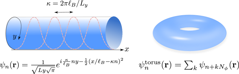
Figure 2: (Color online) Boundary conditions considered in this paper, compatible with Landau gauge: cylinder (left) and torus (right). The associated single-particle states $\psi_{n}(\mathbf{r})$ are arranged along a 1D chain, with the parameter $\kappa=2\pi\ell_{B}/L_{y}$ controlling the distance between nearest neighbor orbitals.

Under periodic boundary conditions (PBCs) in one direction (say $\hat{y}$), the single-particle Hilbert space is spanned by the Landau gauge basis wave function labelled by $n$:

$$\psi_{n}(x,y)\equiv\langle\vec{r}|c_{n}^{\dagger}\left|0\right\rangle\propto e^{i\frac{\kappa}{\ell_{B}}ny}e^{-\frac{1}{2}\left(\frac{x}{\ell_{B}}-\kappa n\right)^{2}},$$ (8)

where $\ell_{B}=\sqrt{\hbar/eB}$ is the magnetic length and $c_{n}^{\dagger}$ is the second-quantized operator that creates a particle in the state $|n\rangle$. The parameter $\kappa=2\pi\ell_{B}/L_{y}$ sets the effective separation between the one-body states in the $x$-direction, as each one-body state is a Gaussian packet approximately localized around $\kappa n$ in $x$-direction (Fig. 2).

Due to this simple one-parameter labeling of the one-body states, an $N$-body interaction matrix element is labeled by $2N$ indices. Additional constraints on its functional form arise when we consider interactions projected to a given Landau level (Fig. 3). Due to the magnetic translation invariance, the interactions projected to a Landau level only allow for scattering that conserves total momentum, or equivalently leaves the COM of the particles fixed. For example, the process in Fig. 3a is allowed, but the one in Fig. 3b is forbidden. This special structure in the interaction Hamiltonian gives rise to the symmetry under many-body translations that shifts every particle by $q$ orbitals at filling $\nu=p/q$ (Fig. 3c). This is the symmetry that underlies the topological ground state degeneracy.

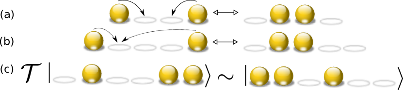
Figure 3: (Color online) Scattering schemes and symmetries in a Landau level. Preservation of COM allows a cluster of particles to scatter according to (a), but forbids the scattering according to (b). (c) The many-particle translation operator $\hat{T}$ acts on a given configuration by moving every particle $q$ orbitals to the right (in this example, $q=2$). Many-body states at filling $\nu=p/q$ are invariant under this symmetry, which gives rise to the topological degeneracy equal to $q$.

The matrix elements of any interaction $V({\mathbf{r}}_{1},...,{\mathbf{r}}_{N})$ projected to a Landau level are given by

$$V_{\{n_{j}\},\{n^{\prime}_{j}\}} = \int d{\mathbf{r}}_{1}\ldots d{\mathbf{r}}_{N}$$ (9)

$$\left(\prod_{j}\psi^{*}_{n^{\prime}_{j}}({\mathbf{r}}_{j})\psi_{n_{j}}({\mathbf{r}}_{j})\right)V({\mathbf{r}}_{1},...,{\mathbf{r}}_{N}),$$

which corresponds to the second-quantized Hamiltonian

$$H=\sum_{\alpha}\sum_{n}b^{\alpha\dagger}_{n}b^{\alpha}_{n},$$

$$b^{\alpha}_{n}\propto\sum_{\sum_{j}n_{j}=n}p_{\alpha}(\kappa\bar{n}_{1},...,\kappa\bar{n}_{N})e^{-\frac{\kappa^{2}}{2}\sum_{j=1}^{N}\bar{n}_{j}^{2}}c_{n_{1}}\ldots c_{n_{N}}.$$

(10)

Here $\bar{n}_{j}=n_{j}-n/N$ denotes the orbital of particle $j$ with respect to the COM, $n=n_{1}+...+n_{N}$, and $p_{\alpha}$ is a polynomial in $N$ variables $\kappa\bar{n}_{j}$. The index $\alpha$, as will be clear from the explicit construction of $p_{\alpha}$ below, specifies the degree of the polynomial and, for a multicomponent state discussed in Section IV, its spin sector. The polynomial $p_{\alpha}$ can be chosen to be real, as will be evident from its geometric construction to follow. From now on, $n$ will refer to the COM, and not the index of a single particle previously appearing in Eq. 8. $c_{n_{j}}^{\dagger}$ is the same operator as in Eq. 8, creating the $j$th particle in state $|n_{j}\rangle$. The Hamiltonian thus consists of a product sum over all positions of the COM $n$, as well as all polynomial degrees $\alpha$.

Eqs. 9 and 10 represent a general translationally invariant Hamiltonian projected to a Landau level. This Hamiltonian has a rather special form: it decomposes into a linear combination of positive-definite operators $b^{\alpha\dagger}_{n}b^{\alpha}_{n}$, such that the form factor $p_{\alpha}e^{-\frac{\kappa^{2}}{2}\sum_{j=1}^{N}\bar{n}_{j}^{2}}$ in each $b^{\alpha}_{n}$ depends only on the relative coordinates of particles. Any short-range Hamiltonian can be explictly expressed in this form Lee and Leinaas (2004); Seidel et al. (2005); Lee et al. (2013), which reveals its Laplacian structure.

Physically, Landau-level-projected Hamiltonians can be visualized as a long-range interacting 1D chain [Fig. 3]. The interaction terms can be interpreted as long-range (though Gaussian suppressed) hopping processes labeled by $\alpha$. For each $\alpha$, $N$ particles “hop” from sites $n_{j}$ to sites $n^{\prime}_{j}$, $j=1,...,N$ according to a COM independent amplitude given by $p_{\alpha}(\kappa\bar{n}_{1},...,\kappa\bar{n}_{N})e^{-\frac{\kappa^{2}}{2}\sum_{j=1}^{N}\bar{n}_{j}^{2}}$, such that the initial and final COM $n$ remains unchanged (Fig. 3c). Note that although we use the term “hopping”, there is no clear distinction between “hopping” and “interaction” in our case, as opposed to the Hubbard model. Rather, “hopping” is designated for any interaction term that is purely quantum (i.e., not of Hartree form). The goal of the remainder of this paper is to show how to systematically construct the polynomial amplitudes $p_{\alpha}$ that need to be inserted into Eq. (10) to obtain the parent Hamiltonian for the desired quantum Hall state.

III.2 Geometric derivation

We now specialize Eq. 9 to $N$-body interactions that are Haldane PPs $U^{N}_{m}$. One appealing feature of the second-quantized form of Eq. 9 is that we can construct the desired PPs from symmetry principles alone, without referring to the first-quantized form of the interaction $V(\mathbf{r}_{1},...,\mathbf{r}_{N})$.

The many-body PPs are, by definition, supposed to project onto orthogonal subspaces labeled by $m$, where $m$ denotes the relative angular momentum:

$$U^{N}_{m^{\prime}}U^{N}_{m}=\left|\psi^{N}_{m^{\prime}}\right\rangle\left\langle\psi^{N}_{m^{\prime}}\right|\left|\psi^{N}_{m}\right\rangle\left\langle\psi^{N}_{m}\right|=U^{N}_{m}\delta_{m^{\prime}m}.$$ (11)

This requires that

$$\left\langle 0\right|b^{m^{\prime}\dagger}_{n}b^{m}_{n}\left|0\right\rangle \propto \sum_{\bar{n}_{1}+...+\bar{n}_{N}=0}p_{m^{\prime}}(\kappa\bar{n}_{1},...,\kappa\bar{n}_{N})$$ (12)

$$\times p_{m}(\kappa\bar{n}_{1},...,\kappa\bar{n}_{N})\exp{\left(-\kappa^{2}\sum_{j=1}^{N}\bar{n}_{j}^{2}\right)}$$

$$= \delta_{m^{\prime}m}.$$

If $\psi^{N}_{m}$ is to vanish with $m$th total power as $N$ particles approach each other, the polynomial $p_{m}$ must be of degree $m$. Hence the PPs will be completely determined once we find a set of polynomials $\{p_{m}\}$ such that: (1) $p_{m}$ is of total degree $m$; (2) $p_{m}$ has the correct symmetry property under exchange of particles, i.e. is totally (anti)symmetric for bosonic (fermionic) particles; (3) the $p_{m}$’s are orthonormal under the inner product measure

$$\langle p_{m^{\prime}},p_{m}\rangle = \sum_{\bar{n}_{1}+...+\bar{n}_{N}=0}p_{m^{\prime}}(\kappa\bar{n}_{1},...,\kappa\bar{n}_{N})$$ (13)

$$\times p_{m}(\kappa\bar{n}_{1},...,\kappa\bar{n}_{N})\exp\left(-\kappa^{2}\sum_{j=1}^{N}\bar{n}_{j}^{2}\right).$$

Using the barycentric coordinates (Appendix A) to represent the tuple $(\bar{n}_{1},...,\bar{n}_{N})$

$$\langle p_{m^{\prime}},p_{m}\rangle \approx \int_{\mathbb{R}^{N-1}}dWd\Omega\;\;p_{m^{\prime}}(W,\Omega)p_{m}(W,\Omega)$$ (14)

$$\times \exp{(-\frac{N-1}{N}W^{2})}J_{N-1}(W,\Omega)$$

$$= \delta_{m^{\prime}m},$$

where $W$ and $\Omega$ are the radial and angular coordinates of the vector $\vec{x}\in\mathbb{R}^{N-1}$ representing the tuple $(\bar{n}_{1},...,\bar{n}_{N})$, and $J_{N-1}$ is the Jacobian for the spherical coordinates in $\mathbb{R}^{N-1}$. We have exploited the magnetic translation symmetry of the problem in quotienting out the COM coordinate $n$. (It is desirable to quotient out $n=\sum_{j}^{N}n_{j}$, since $n$ takes values on an infinite set when the particles lie on the 2D infinite plane, and that complicates the definition of the inner product measure.) Each quotient space is most elegantly represented as an $N-1$-simplex in barycentric coordinates, where particle permutation symmetry (or subgroups of it) is manifest. Explicitly, the set of $\bar{n}_{j}$ can be encoded in the vector

$$\vec{x}=\kappa\sum_{j=1}^{N}\bar{n}_{j}\vec{\beta}_{j},$$ (15)

where the $N$ basis vectors $\{\vec{\beta}_{j}\}$ form a set that spans $\mathbb{R}^{N-1}$. A configuration $(\bar{n}_{1},...,\bar{n}_{N})$ is uniquely represented by a point $\vec{x}\in\mathbb{R}^{N-1}$ that is independent of $n=\sum_{j}^{N}n_{j}$. Since $\vec{x}$ should not favor any particular $\bar{n}_{j}$, any pair of vectors in the basis $\{\vec{\beta}_{j}\}$ must form the same angle with each other. Specifically,

$$\vec{\beta}_{j}\cdot\vec{\beta}_{k}=\frac{N}{N-1}\delta_{jk}-\frac{1}{N-1},$$ (16)

so that each vector points at the angle of $\pi-\cos^{-1}\frac{1}{N-1}$ from another.

With this parametrization, the Gaussian factor reduces to the simple form

$$W^{2}=|\vec{x}|^{2}=\frac{N}{N-1}\kappa^{2}\sum_{j=1}^{N}\bar{n}_{j}^{2}.$$ (17)

Further mathematical details can be found in the examples that follow, as well as in Appendix A.

The integral approximation in Eq. 14 becomes exact in the infinite plane limit, and is still very accurate for values of $m$ where the characteristic inter-particle separation is smaller than the smallest of the two linear dimensions of the QH system. In the following, we will assume this to be the case; otherwise, there can be significant effects from the interaction of a particle with its periodic images. This was systematically studied in the appendix of Ref. Lee et al., 2013 for $N=2$. We note that the approximation in Eq. 14 does not affect the exact zero mode property of the trial Hamiltonians constructed below.

III.3 Orthogonalization

We are now ready to evaluate the pseudopotentials. To find a second-quantized PPs with relative angular momentum $m$, one needs to follow the rules listed in Table 1.

(1) Write down the allowed “primitive” polynomials Simon et al. (2007b, a); Davenport and Simon (2012) of degree $m^{\prime}\leq m$ consistent with the symmetry of the particles.

(2) Orthogonalize this set of primitive polynomials according to the inner product measure in Eq. 14.

Table 1: Summary of the PP construction for spinless particles. Examples of this procedure are given in Sec. V.

In the following, we shall execute this recipe explicitly for $N=2,3$, and, to some extent, $N=4$-body interactions.

III.3.1 $2$-body case

For two-body interactions, we have

$$\langle p_{m^{\prime}},p_{m}\rangle=\int_{-\infty}^{\infty}p_{m^{\prime}}(W)p_{m}(W)e^{-\frac{1}{2}W^{2}}dW,$$ (18)

where $W=-2\kappa\bar{n}_{1}=2\kappa\bar{n}_{2}$. For this $N=2$ case, we have allowed $W$ to take negative values as the angular direction spans the 1D circle, which consists of just two points. The primitive polynomials for bosons are $\{1,W^{2},W^{4},W^{6},...\}$ while those for fermions are $\{W,W^{3},W^{5},...\}$. After performing the Gram-Schmidt orthogonalization procedure, the $2$-body PPs are found to be $U^{2}_{m}\propto\kappa^{3}\sum_{n}b^{m\dagger}_{n}b^{m}_{n}$, where

$$b^{m}_{n}=\sum_{\bar{n}_{1}+\bar{n}_{2}=0}p_{m}(\kappa\bar{n}_{1},\kappa\bar{n}_{2})e^{-\frac{1}{2}\kappa^{2}(\bar{n}_{1}^{2}+\bar{n}_{2}^{2})}c_{n/2+\bar{n}_{1}}c_{n/2+\bar{n}_{2}},$$ (19)

$n/2+\bar{n}_{j}$ are integers, and $p_{m}$ is a $m$th degree Hermite polynomial given in Table 2. In particular, we recover the Laughlin $\nu=1/2$ bosonic or $\nu=1/3$ fermionic state for $m=0$ or $m=1$ respectively.

$m$	Bosonic $p_{m}(W)$	Fermionic $p_{m}(W)$
0	$1$	0
1	$0$	$W$
2	$\frac{1}{\sqrt{2!}}(-1+W^{2})$	0
3	$0$	$\frac{1}{\sqrt{3!}}(-3+W^{2})W$
4	$\frac{1}{\sqrt{4!}}(3-6W^{2}+W^{4})$	0
5	$0$	$\frac{1}{\sqrt{5!}}(15-10W^{2}+W^{4})W$
6	$\frac{1}{\sqrt{6!}}(-15+45W^{2}$	$0$
	$-15W^{4}+W^{6})$
7	$0$	$\frac{1}{\sqrt{7!}}(-105+105W^{2}-21W^{4}$
		$+W^{6})W$

Table 2: Representative polynomials $p_{m}$ for the first few $N=2$-body PPs for bosons and fermions. $p_{m}(W)e^{-W^{2}/4}$ represents the amplitude that two particles $W/\kappa$ sites apart are involved in a two-body hopping on the chain.

One can easily check that PPs become more delocalized in $W$-space as $m$ increases. Indeed,

$$\kappa^{2}\langle\sum_{j}\bar{n}_{j}^{2}\rangle = \frac{1}{2}\langle W^{2}\rangle=\frac{1}{2}\int_{-\infty}^{\infty}p_{m}(W)W^{2}e^{-\frac{1}{2}W^{2}}dW$$ (20)

$$= m+\frac{1}{2},$$

which is reminiscent of the interpretation of $m$ as the angular momentum of a pair of particles in rotationally-invariant geometries (Fig. 1). Obtaining the pseudopotentials in this second-quantized form is highly advantageous. In particular, note that this construction is free from ambiguities in the choice of $V(\mathbf{r}_{1},...,\mathbf{r}_{N})$, since several possible real-space interactions, e.g., those of the Trugman-Kivelson type Trugman and Kivelson (1985), can all be grouped into the same $m$ sector. This is discussed in more detail in Appendix B.

III.3.2 $3$-body case

For $N=3$, the inner product measure takes the form

$$\langle p_{m^{\prime}},p_{m}\rangle=\int_{0}^{\infty}\int_{0}^{2\pi}p_{m^{\prime}}(W,\theta)p_{m}(W,\theta)e^{-\frac{2}{3}W^{2}}Wd\theta dW$$ (21)

with

$$\bar{n}_{1} =\frac{2W}{3\kappa}\cos\theta$$ (22a)

$$\bar{n}_{2} =\frac{W}{3\kappa}(\sqrt{3}\sin\theta-\cos\theta)$$ (22b)

$$\bar{n}_{3} =\frac{W}{3\kappa}(-\sqrt{3}\sin\theta-\cos\theta)$$ (22c)

Each of the $\bar{n}_{j}$’s are treated on equal footing, as one can easily check graphically. The above expressions are the simplest nontrivial cases of the general expressions for barycentric coordinates found in the Appendix (Eqs. 62-64).

The bosonic primitive polynomials are made up of elementary symmetric polynomials $S_{1},S_{2},S_{3}$ in the variables $\kappa\bar{n}_{j}=\kappa(n_{j}-n/N)$. Since $S_{1}=\kappa\sum_{j}\bar{n}_{j}=0$, the only two symmetric primitive polynomials are

$$-S_{2}=-\kappa^{2}\sum_{i<j}\bar{n}_{i}\bar{n}_{j}=\frac{S_{1}^{2}-2S_{2}}{2}=\frac{\kappa^{2}}{2}\sum_{i}\bar{n}_{i}^{2}=\frac{1}{3}W^{2},$$ (23)

and

$$Y=S_{3} = \kappa^{3}\prod_{i}\bar{n}_{i}$$ (24)

$$= \frac{\kappa^{3}}{27}(2n_{1}-n_{2}-n_{3})(2n_{2}-n_{3}-n_{1})$$

$$(2n_{3}-n_{1}-n_{2})$$

$$= \frac{2}{27}W^{3}\cos 3\theta.$$

The fermionic primitive polynomials are totally antisymmetric, and can always be writtenSimon et al. (2007b); Davenport and Simon (2012) as a symmetric polynomial multiplied by the Vandermonde determinant

$$A = \kappa^{3}(n_{1}-n_{2})(n_{2}-n_{3})(n_{3}-n_{1})$$ (25)

$$= \kappa^{3}(\bar{n}_{1}-\bar{n}_{2})(\bar{n}_{2}-\bar{n}_{3})(\bar{n}_{3}-\bar{n}_{1})$$

$$= -\frac{2}{3\sqrt{3}}W^{3}\sin 3\theta.$$

Note that $W^{2}$ is of degree 2 while $A$ and $Y$ are of degree 3. All of them are independent of the COM coordinate $n$, as they should be. $N=3$ PPs were derived in Ref. Lee et al., 2013 through explicit integration, and the approach discussed here considerably simplifies those computations by exploiting symmetry.

To generate the fermionic (bosonic) PPs up to $U^{3}_{m}$, we need to orthogonalize the basis consisting of all possible (anti)symmetric primitive polynomials up to degree $m$. For instance, the first seven (up to $m=9$) 3-body fermionic PPs are generated from the primitive basis $\{A,AW^{2},AY,AW^{4},AYW^{2},AY^{2},AW^{3}\}$. Note that the last two basis elements both contribute to the $m=9$ PP sector.

The 3-body PPs are found to be $U^{3}_{m}\propto\kappa^{3}\sum_{n}b^{m\dagger}_{n}b^{m}_{n}$, where

$$b^{m}_{n}=\sum_{n_{1}+n_{2}+n_{3}=n}p_{m}(W,Y,A)e^{-\frac{1}{3}W^{2}}c_{n_{1}}c_{n_{2}}c_{n_{3}},$$ (26)

with the polynomials $p_{m}$ listed in Table 3. These results are fully compatible with those from Ref. Simon et al., 2007b. As mentioned, there can be more than one (anti)symmetric polynomial of the same degree for sufficiently large $m$. This leads to the degenerate PP subspace, a specific example of which is presented in Sec. V.1.2.

$m$	Bosonic $p_{m}(W,Y)$	Fermionic $p_{m}(W,Y,A)$
0	$1$	0
1	$0$	0
2	$1-\frac{2}{3}W^{2}$	0
3	$3\sqrt{2}Y$	$A$
4	$1-\frac{4}{3}W^{2}+\frac{2}{9}W^{4}$	0
5	$\sqrt{2}Y(6-W^{2})$	$A\left(2-\frac{1}{3}W^{2}\right)$
6	(i) $1-2W^{2}+\frac{2}{3}W^{4}-\frac{4}{81}W^{6}$ (ii) $\frac{1}{81}\sqrt{\frac{2}{5}}(2W^{6}-729Y^{2})$	$\frac{3}{\sqrt{5}}AY$
7	$\frac{2}{3\sqrt{5}}(45-15W^{2}+W^{4})Y$	$\sqrt{10}A\left(1-\frac{1}{3}W^{2}+\frac{1}{45}W^{4}\right)$
8	(i) $1+\frac{2}{243}W^{2}(W^{2}-6)(54-18W^{2}+W^{4})$	$3\sqrt{\frac{7}{5}}\left(1-\frac{2}{21}W^{2}\right)AY$
	(ii) $\frac{1}{243}\sqrt{\frac{2}{35}}(2W^{2}-21)(2W^{6}-729Y^{2})$
9	(i) $\sqrt{\frac{6}{155}}Y(-30+15W^{2}-2W^{4}+18Y^{2})$ (ii) $\frac{1}{27}\sqrt{\frac{2}{1085}}Y(-5760W^{2}+756W^{4}-31W^{6}+81(140+9Y^{2}))$	(i) $\frac{A}{\sqrt{5}}(-10+5W^{2}-\frac{2}{3}W^{4}+\frac{2}{81}W^{6})$ (ii) $\frac{A}{81\sqrt{105}}\left(W^{6}-729Y^{2}\right)$

Table 3: The polynomials $p_{m}$ for $N=3$-body PPs for bosons and fermions up to $m=9$. Note that there is more than one possible PP for larger $m$, since there are multiple ways to build a homogeneous (anti)symmetric polynomial from the primitive and elementary symmetric polynomials. For instance, with $Y$ and $A$ defined in Eqs. 24 and 25, there are two possible bosonic PPs for $m=6$, since there are two ways ($W^{6}$ and $Y^{2}$) to build a homogeneous 6-degree polynomial from elementary symmetric polynomials. For the fermionic cases, we have explicitly kept only one factor of $A$, since even powers of $A$ can be expressed in terms of $W^{2}$ and $Y$. For all cases, the mean-square spread of the PPs also increases linearly with $m$, i.e. $\kappa^{2}\langle\sum_{j}^{3}\bar{n}_{j}^{2}\rangle=m+1$ (compare with the two-body case in Eq. 20).

III.3.3 $N\geq 4$-body case

For general PPs involving $N$ bodies, the inner product measure takes the form

$$\langle p_{m^{\prime}},p_{m}\rangle = \int_{0}^{\infty}e^{-\frac{N-1}{N}W^{2}}W^{N-2}dW$$

$$\times\int_{0}^{2\pi}d\phi_{N-2}\prod_{k=1}^{N-3}\int_{0}^{\pi}\sin^{N-2-k}(\phi_{k})d\phi_{k}$$

$$\times p_{m^{\prime}}(W,\phi_{1},...,\phi_{N-2})p_{m}(W,\phi_{1},...,\phi_{N-2}),$$

where the Jacobian determinant from Eq. 14 has already been explicitly included. One transforms the tuple $\{\bar{n}_{1},...,\bar{n}_{N}\}$ into $(N-1)$-dim spherical coordinates via the barycentric coordinates detailed in Appendix A.

The bosonic primitive basis is spanned by the elementary symmetric polynomials $\{S_{2},S_{3},...,S_{N}\}=\{\sum_{ij}\bar{n}_{i}\bar{n}_{j},\sum_{ijk}\bar{n}_{i}\bar{n}_{j}\bar{n}_{k},...,\prod_{j}\bar{n}_{j}\}$ and combinations thereof. For instance, with $N=5$ particles at degree $m=6$, there are $3$ possible primitive polynomials: $S_{2}^{3},S_{3}^{2}$ and $S_{2}S_{4}$. The fermionic primitive basis is spanned by all the symmetric polynomials as above, times the degree $\binom{N}{2}$ Vandermonde determinant $\prod_{i<j}(\bar{n}_{i}-\bar{n}_{j})$ shown in Fig. 4.

From the examples above, one easily deduces the degeneracy of the PPs $U^{N}_{m}$ to be $P(m,N)-P(m-1,N)$ for bosons and $P\left(m-\binom{N}{2},N\right)-P\left(m-1-\binom{N}{2},N\right)$ for fermions, where $P(m,N)$ is the number of partitions of the integer $N$ into at most $m$ partsSimon et al. (2007b); Davenport and Simon (2012). In particular, the degeneracy is always nontrivial ($\geq 2$) whenever $N\geq 4$ and $m\geq 4$.

Figure 4: (Color online) The primitive polynomials have beautiful geometric shapes when plotted in $N-1$-dim spherical coordinates. Shown above are the constant $W$ plots of the antisymmetric polynomial $A=(\bar{n}_{1}-\bar{n}_{2})(\bar{n}_{1}-\bar{n}_{3})(\bar{n}_{1}-\bar{n}_{4})(\bar{n}_{2}-\bar{n}_{3})(\bar{n}_{2}-\bar{n}_{4})(\bar{n}_{3}-\bar{n}_{4})$ (left), and the degree $m=4$ symmetric expression in the orthonormalized space spanned by the elementary symmetric polynomials $1,S_{2},S_{3},S_{4}$ and $S^{2}_{2}$ (right). On the left, there are $24$ lobes that each maximally avoid the vertices of the tetrahedron (3-simplex). On the right, the $6$ lobes lie around the centers of the $6$ edges of the tetrahedron, where two of the $\bar{n}_{i}$’s are equal.

IV Geometric construction of pseudopotentials: spinful case

In the presence of “internal degrees of freedom” (DOFs) which we also refer to as “spins” or “components” for simplicity, there are considerably more possibilities for the diverse forms of the PPs. This is because the PPs consist of products of spatial and spin parts, and either part can have many possible symmetry types, as long as they conspire to produce an overall (anti)symmetric PP in the case of (fermions) bosons.

A generic multicomponent PP takes the form

$$U^{N}_{m}=\sum_{\lambda}\sum_{\sigma}U^{N}_{m,\lambda}\left|\sigma^{\lambda}\right\rangle\left\langle\sigma^{\lambda}\right|.$$ (28)

The notation here requires some explanation. $\lambda=[\lambda_{1},\lambda_{2},...]$ defines a partition of all particles into several subgroups $\lambda_{i}$ each of which imposing a symmetry constraint among particles of this subgroup. Associated with it is $U^{m}_{\lambda}$ which is a spatial term (in $(\bar{n}_{1},...,\bar{n}_{N})$-space) exhibiting this symmetry. $\left|\sigma^{\lambda}\right\rangle=\left|\sigma_{1}\sigma_{2}...\right\rangle$ refers to an (internal) spin basis that is consistent with the symmetry type $\lambda$. Each symmetry type corresponds to a partition of $N$, with $\sum_{j}\lambda_{j}=N$. For $N$ bosons, $\lambda$ represents the situation where there is permutation symmetry among the first $\lambda_{1}$ particles, among the next $\lambda_{2}$ particles, etc. but no additional symmetry between the $\lambda_{i}$ subsets. This is often represented by the Young Tableau with $\lambda_{i}$ boxes in the $i^{th}$ row. For fermions, we use the conjugate representation $\bar{\lambda}$, with the rows replaced by columns and symmetry conditions replaced by antisymmetry ones. For instance, the totally (anti)symmetric types are $[1,1,...,1]$ and $[N]$, respectively.

Hence the space of PPs is specified by three parameters: $N$ – the number of particles interacting with each other, $m$ – the total relative angular momentum or the total polynomial degree in $\bar{n}_{i}$, and $b$ – the number of internal DOFs (spin). While the symmetry type $\lambda$ and hence $U^{N}_{m,\lambda}$ depends only on $N$ and $m$, the set of possible $\left|\sigma^{\lambda}\right\rangle$ also depends on $b$. To further illustrate our notation, we specify $N,m,b$ parameters for the interactions relevant to some commonly known states: in the archetypical single-layer FQH states, we have $b=1$ components, and the $N=2$ PP interactions for the Laughlin state penalize pairs of particles with relative angular momentum $m$, where $\frac{1}{m+2}$ is the filling fraction. For bilayer FQH states, we have $b=2$ and $N=2$-body interactions. PPs as energy penalties in the $[2]$ sector with angular momentum $<m$ and $[1,1]$ sectors with angular momentum $<n$ give rise to the Halperin $(mmn)$ states. Here, the $[2]$ sector is also known as the triplet channel, as it is spanned by the following three basis vectors: $\{\left|\uparrow\uparrow\right\rangle,\left|\uparrow\downarrow\right\rangle+\left|\downarrow\uparrow\right\rangle,\left|\downarrow\downarrow\right\rangle\}$. By contrast, the $[1,1]$ sector only contains $\{\left|\uparrow\downarrow\right\rangle-\left|\downarrow\uparrow\right\rangle\}$ as dictated by antisymmetry.

IV.1 Multicomponent pseudopotentials for a given symmetry

The construction of multicomponent PPs here parallels that of multicomponent wave functions described in Ref. Davenport and Simon, 2012. For completeness, we first review this construction, and proceed to show how an orthonormal multicomponent PP basis, adapted to the cylinder or torus, can be explicitly found through the geometric approach. We describe how to first find the spatial part of the PP $U^{N}_{m,\lambda}$, and second the spin basis $\left|\sigma^{\lambda}\right\rangle$.

IV.1.1 Spatial part

For each symmetry type $\lambda$, we can construct the spatial part $U^{N}_{m,\lambda}$ with elementary symmetric polynomials in subsets of the particle indices $\bar{n}_{i}=n_{i}-n/N$. They are, for instance, $S_{1,12}=\bar{n}_{1}+\bar{n}_{2}$, $S_{2,234}=\bar{n}_{2}\bar{n}_{3}+\bar{n}_{3}\bar{n}_{4}+\bar{n}_{2}\bar{n}_{4}$, etc. Of course, we must have $S_{1,123...N}=\sum_{i}\bar{n}_{i}=0$.

Like in the single-component case, the spatial part $U^{N}_{m,\lambda}$ consists of a primitive polynomial which enforces the symmetry, and a totally symmetric factor that does not change the symmetry. Here, the main step in the multicomponent generalization is the replacement of primitive polynomials $1$ and $A$ by primitive polynomials consistent with the symmetry type $\lambda$. As the simplest example, the primitive polynomial in $U^{N=3}_{m=1,[2,1]}$ is $S_{1,12}=-\bar{n}_{3}$ (and cyclic permutations). It is the only possible degree $m=1$ expression symmetric in two (but not all three) of the indices.

In general, there can be more than one candidate monomial obeying a symmetry consistent with $\lambda$. For instance, for $U^{N=3}_{m=2,[2,1]}$ they are $S_{1,12}^{2}=(\bar{n}_{1}+\bar{n}_{2})^{2}$ and $S_{2,12}=\bar{n}_{1}\bar{n}_{2}$ (and cyclic permutations thereof). To find the primitive polynomials, we will have to construct one or more linear combinations of these terms which do not have any higher symmetry other than $[2,1]$ (i.e. in this case, this higher symmetry channel could be $[3]$). Elementary computation reveals that the only primitive polynomial should be $S_{1,12}^{2}+2S_{2,12}$, because it is the only linear combination that is manifestly symmetric in indices $1,2$ and disappears upon symmetrization over all three particles.

$N=4$, $m=2$, $\lambda=[2,2]$. As a more involved example, we demonstrate how to find the primitive polynomial corresponding to the symmetry type $[2,2]$. Independent monomials that satisfy this symmetry include $S_{1,12}^{2}$, $S_{2,12}$ and $S_{2,34}$. The primitive polynomial is then given by the linear combination

$$S_{1,12}^{2}+\mu_{1}S_{2,12}+\mu_{2}S_{2,34}$$ (29)

with $\mu_{1}$ and $\mu_{2}$ to be determined by demanding that the linear combination disappears upon symmetrizing over permutations under $[3,1]$ and $[4]$. The symmetrized sums are

$$2((n_{2}+n_{3})^{2}+(n_{2}+n_{4})^{2}+(n_{3}+n_{4})^{2}+$$

$$\mu_{1}(n_{1}n_{2}+n_{1}n_{3}+n_{2}n_{3})+\mu_{2}(n_{1}n_{4}+n_{2}n_{4}+n_{3}n_{4}))$$

and

$$4\left(n_{2}^{2}+n_{3}^{2}+n_{4}^{2}+n_{2}n_{3}+n_{3}n_{4}+n_{2}n_{4}\right)(4-\mu_{1}-\mu_{2}).$$

Setting them both to zero, we find $\mu_{1}=\mu_{2}=2$, so the primitive polynomial is $S_{1,12}^{2}+2S_{2,12}+2S_{2,34}$.

$N=3$, $m=2$, $\lambda=[2,1]$. The above procedure works for arbitrarily complicated cases, but quickly becomes cumbersome. This is when our geometric approach again becomes useful. We first write down the relevant monomials in barycentric coordinates given by Eq. 22 for $N=3$ bodies (or Eq. 71 for general $N$). The coefficients in the primitive polynomial can then be elegantly determined through graphical inspection. We demonstrate this explicitly by revisiting the example on $\lambda=[2,1]$. Recall that the primitive polynomial (call it $\beta_{m=2}\equiv\beta_{2}$) is a linear combination of $S_{1,12}^{2}$ and $S_{2,12}$, i.e.

$$\beta_{2} = S_{1,12}^{2}+\mu S_{2,12}$$

$$= -\frac{W^{2}}{9\kappa}\left(\mu-2+(1+\mu)(\cos 2\theta-\sqrt{3}\sin 2\theta)\right)$$

where $\theta=0,2\pi/3,4\pi/3$ points towards the vertices favoring $\bar{n}_{1},\bar{n}_{2},\bar{n}_{3}$ respectively. The correct value of $\mu$ will cause $\beta_{2}$ to disappear under symmetrization of the $3$ particles. Graphically, it means that the lobes of three copies of the plot of $\beta_{2}$, each rotated an angle $2\pi/3$ from each other, must cancel upon addition. This is illustrated in Fig. 5, where $\mu=2$ is readily identified as the correct value.

Figure 5: (Color online) Polar plots of $\beta_{2}(\theta)$ as a function of $\theta$, with $\mu=0.5$ (blue curve) and $\mu=2$ (purple curve). $\beta_{2}(\theta)+\beta_{2}(\theta+2\pi/3)+\beta_{2}(\theta+4\pi/3)$ sum to zero only when the lobes are of equal size, which is the case for $\mu=2$ only.

All in all, we have the $m=2$ primitive polynomial for $[2,1]$:

$$\beta_{2}=(\bar{n}_{3})^{2}+2\bar{n}_{1}\bar{n}_{2}=\frac{W^{2}}{3}\left(-\cos 2\theta+\sqrt{3}\sin 2\theta\right).$$ (33)

$N=3$, $m=1$, $\lambda=[2,1]$. The reader is invited to also visualize the simpler case for the $[2,1]$ sector, which takes the form

$$\beta_{1}=S_{1,12}=-\bar{n}_{3}=\frac{W}{3\kappa}\left(\cos\theta+\sqrt{3}\sin\theta\right).$$ (34)

Compared to the antisymmetric case for fermions, we have two primitive polynomials $\beta_{1},\beta_{2}$, instead of just $A$. The primitive polynomials for a wide variety of cases are also listed in Table II and III of Ref. Davenport and Simon, 2012, and can alternatively be systematically derived via the theory of Matric units explained in the appendix of the same reference.

IV.1.2 Admissible spin bases

In general, not all possible $N$-particle spin bases survive under symmetrization with respect to a given symmetry type $\lambda$. Only those that survive should be included, i.e. are admissible, in the set of basis in $\left|\sigma^{\lambda}\right\rangle$. For instance, the basis $\left|\alpha\alpha\alpha\right\rangle$ does not appear in $\left|\sigma^{[2,1]}\right\rangle$. To see this, try symmetrizing the combination $p(\bar{n}_{1},\bar{n}_{2},\bar{n}_{3})\left|\alpha\alpha\alpha\right\rangle$ subject to the condition that $p(\bar{n}_{1},\bar{n}_{2},\bar{n}_{3})$ has no higher symmetry than $\lambda=[2,1]$, i.e. the totally symmetrized sum $\mathcal{S}\left[p(\bar{n}_{1},\bar{n}_{2},\bar{n}_{3})\right]=0$. Obviously, $p(\bar{n}_{1},\bar{n}_{2},\bar{n}_{3})\left|\alpha\alpha\alpha\right\rangle$ then has to symmetrize to zero and should not be included in $[2,1]$.

There is a nice way to write down the set of admissible bases by looking at the labelings of semistandard Young Tableaux. From Ref. Davenport and Simon, 2012, the admissible bases in $\left|\sigma^{\lambda}\right\rangle$, up to permutations, are in one-to-one correspondence with the labelings of semistandard Young Tableaux with numbers $1$ to $N$. (A semistandard Young Tableau has non-decreasing entries along each row and strictly increasing entries along each column.) For instance, a symmetry type of $[3,1]$ with $b=3$ corresponds to labelings (with labels $a,b,c$ defined to be in increasing order):

$$[aaa,b],\;[aab,b],\;[aac,b],\;[abb,b],\;[abc,b],$$

$$[acc,b],\;[aaa,c],\;[aab,c],\;[aac,c],[abb,c],$$

$$[abc,c],\;[acc,c],\;[bbb,c],\;[bbc,c],\;[bcc,c]\;{\rm and}\;[ccc,c],$$

where rows are separated by commas. From these, the admissible states for $\lambda=[3,1]$ can be written down by copying the labelings verbatim:

$$\left|aaab\right\rangle,\;\left|aabb\right\rangle,\;\left|aacb\right\rangle,\;\left|abbb\right\rangle,\;\left|abcb\right\rangle,$$

$$\left|accb\right\rangle,\;\left|aaac\right\rangle,\;\left|aabc\right\rangle,\;\left|aacc\right\rangle,\;\left|abbc\right\rangle,$$

$$\left|abcc\right\rangle,\;\left|accc\right\rangle,\;\left|bbbc\right\rangle,\;\left|bbcc\right\rangle,\;\left|bccc\right\rangle\;{\rm and}\;\left|cccc\right\rangle.$$

In the Young Tableau corresponding to $\lambda$, each row represents a set of particles that are symmetric with each other in the $\lambda$ representation. The requirement that labels increase monotonically within each row defines an ordering, and prevents the repeated listing of basis states related by permutation. The requirement of strictly increasing labelings down each column also prevents that, and also avoids the listing of bases that do not survive under symmetry constraints.

With these preliminary considerations, we are now in position to formulate the general recipe for constructing PPs in the multicomponent case, which is given in Table 4. In the following section we apply this recipe to the case of SU(2) spins with 3-body interactions.

(1) Given $N$,$m$ and $b$, specify which symmetry type the PP is associated with. For example, we specify the $[2]$ or the $[1,1]$ channel when computing PPs realizing the fermionic Halperin states in bilayer QH systems ($b=2,N=2$).
(2) Next, determine the appropriate primitive polynomials by finding the coefficients multiplying the allowed monomials. Then multiply the primitive polynomial by symmetric polynomials, and orthogonalize to obtain the spatial parts $U^{N}_{m,\lambda}$.
(3) Finally, choose the desired admissible spin channels, and (anti)symmetrize the resultant product of the spatial and spin parts depending on whether we want a bosonic (fermionic) PP.

Table 4: Summary of the PP construction procedure for the multicomponent case. Examples of this procedure are given in Section V.

IV.2 Example: $N=3$-body case for SU(2) spins

Here we explicitly work out the multi-component case $b=2$ which is also the most common multi-component scenario. We focus on $N=3$-body interactions to illustrate the nontrivial aspects of our approach.

The symmetry type is given by $[\lambda_{1},\lambda_{2}]=[N/2+S,N/2-S]$, where $S$ is the total spin of the particles. Let us denote the spins by $\uparrow,\downarrow$. There are only $N=3$ boxes in the Young Tableaux, with the following possible symmetry types: $[3]$, $[2,1]$, $[1,1,1]$.

For type $\lambda=[3]$, the possible spin bases are $\left|\uparrow\uparrow\uparrow\right\rangle$, $\left|\uparrow\uparrow\downarrow\right\rangle$, $\left|\uparrow\downarrow\downarrow\right\rangle$ and $\left|\downarrow\downarrow\downarrow\right\rangle$. For $\lambda=[2,1]$, the possible spin bases are $\left|\uparrow\downarrow\downarrow\right\rangle$, $\left|\uparrow\uparrow\downarrow\right\rangle$, corresponding to Tableau labellings $[\uparrow\downarrow,\downarrow]$ and $[\uparrow\uparrow,\downarrow]$ respectively. For $\lambda=[1,1,1]$, there is actually no admissible spin basis: total (internal DOF) antisymmetry is impossible for 3 particles, if there are only 2 different spin states to choose from.

Consider bosonic particles in the following. The symmetry type $[3]$ case corresponds to the primitive polynomial $1$, so the resultant PP takes the same form as in the single-component case. After symmetrizing the spin part, we have the following available sets of spin channels for $[3]$:

$$\{\left|\uparrow\uparrow\uparrow\right\rangle\},$$

$$\{\left|\uparrow\uparrow\downarrow\right\rangle,\left|\uparrow\downarrow\uparrow\right\rangle,\left|\downarrow\uparrow\uparrow\right\rangle\},$$

$$\{\left|\downarrow\downarrow\uparrow\right\rangle,\left|\downarrow\uparrow\downarrow\right\rangle,\left|\uparrow\downarrow\downarrow\right\rangle\},$$

$$\{\left|\downarrow\downarrow\downarrow\right\rangle\}.$$

For the PP $U^{3}_{m,[3]}\propto\kappa^{3}\sum_{n}b^{m\dagger}_{n}b^{m}_{n}$, we have

$$b^{m\dagger}_{n}\left|0\right\rangle=\sum_{\sum_{j}n_{j}=n}p_{m}e^{-\frac{1}{3}W^{2}}\left|\uparrow\uparrow\uparrow\right\rangle\$$ (35)

for $S=3/2$, and

$$b^{\dagger m}_{n}\left|0\right\rangle=\mathcal{S}\left[\sum_{\sum_{j}n_{j}=n}p_{m}e^{-\frac{1}{3}W^{2}}\left|\uparrow\uparrow\downarrow\right\rangle\right]$$ (36)

for $S=1/2$. Other contributions with $S\rightarrow-S$ can be obtained via the identification $\left|\uparrow\right\rangle\leftrightarrow\left|\downarrow\right\rangle$. Here $\left|\uparrow\uparrow\downarrow\right\rangle$ is the shorthand for $c^{\dagger}_{n_{1}\uparrow}c^{\dagger}_{n_{2}\uparrow}c^{\dagger}_{n_{3}\downarrow}\left|0\right\rangle$, etc, and $p_{m}\equiv p_{m,[3]}$ refers to the same polynomial as in the single-component case.

To construct the orthonormal PP basis for the first few $m$, we orthogonalize the set $\{\beta_{1},\beta_{2},\beta_{1}W^{2},\beta_{2}W^{2},\beta_{1}Y,\beta_{2}Y,\beta_{1}W^{4},...\}$. The results are shown in Table 5. Notice that the first PP for symmetry type $[2,1]$ occurs at $m=1$, whereas that of single-component bosons/fermions occur at $m=0$ and $m=3$ respectively. Indeed, there are more ways of constructing PP polynomials when only a subgroup of the full symmetric/alternating group is involved. The onset of PPs degenerate in $m$ also occurs earlier, at $m=4$.

$m$	$p_{m,[2,1]}(\beta_{1},\beta_{2},W,Y)$
1	$\beta_{1}$
2	$\frac{1}{\sqrt{3}}\beta_{2}$
3	$\frac{1}{3}\sqrt{2}\beta_{1}\left(-3+W^{2}\right)$
4(i)	$\frac{1}{\sqrt{5}}\left(\beta_{2}+6\beta_{1}Y\right)$
4(ii)	$\frac{1}{27\sqrt{5}}\left(-54\beta_{2}+12\beta_{2}W^{2}+W^{4}\left(\cos[4\theta]+\sqrt{3}\sin[4\theta]\right)\right)$
5(i)	$\frac{1}{\sqrt{33}}\left(\beta_{1}\left(-3+2W^{2}\right)+6\beta_{2}Y\right)$
5(ii)	$\frac{1}{81}\sqrt{\frac{2}{55}}(-\sqrt{3}W^{5}\cos[5\theta]+3(5\sqrt{3}\beta_{1}(27-18W^{2}$
	$+2W^{4})+W^{5}\sin[5\theta]))$

Table 5: The polynomials $p_{m}$ for the first few $N=3$-body PPs for bosons in the total spin $|S|=\frac{1}{2}$, i.e. $\lambda=[2,1]$ channel. The primitive polynomials $\beta_{1}$ and $\beta_{2}$ are given by Eqs. 33 and 34. $\cos 4\theta,\sin 4\theta,\cos 5\theta,\sin 5\theta$ can all be decomposed into the elementary symmetric polynomials and primitive polynomials $W,Y,\beta_{1}$, and $\beta_{2}$.

To illustrate the full procedure for PP construction with internal DOFs, we detail the case of $S=-1/2$ below. For $m=1$,

$$b^{1\dagger}_{n}\left|0\right\rangle = \mathcal{S}\left[\sum_{\sum_{j}n_{j}=n}(-\bar{n}_{3})e^{-\frac{1}{3}W^{2}}\left|\uparrow\downarrow\downarrow\right\rangle\right]$$

$$= -e^{-\frac{1}{3}W^{2}}[(\bar{n}_{2}+\bar{n}_{3})\left|\uparrow\downarrow\downarrow\right\rangle$$

$$+ (\bar{n}_{1}+\bar{n}_{3})\left|\downarrow\uparrow\downarrow\right\rangle+(\bar{n}_{1}+\bar{n}_{2})\left|\downarrow\downarrow\uparrow\right\rangle]$$

$$= e^{-\frac{1}{3}W^{2}}[\bar{n}_{1}\left|\uparrow\downarrow\downarrow\right\rangle+\bar{n}_{2}\left|\downarrow\uparrow\downarrow\right\rangle+\bar{n}_{3}\left|\downarrow\downarrow\uparrow\right\rangle],$$

while for $m=2$ we have

$$b^{2\dagger}_{n}|0\rangle = \mathcal{S}\left[\sum_{\sum_{j}n_{j}=n}((\bar{n}_{3})^{2}+2\bar{n}_{1}\bar{n}_{2})e^{-\frac{1}{3}W^{2}}\left|\uparrow\downarrow\downarrow\right\rangle\right]$$

$$= e^{-\frac{1}{3}W^{2}}[((\bar{n}_{2})^{2}+(\bar{n}_{3})^{2}+2\bar{n}_{1}(\bar{n}_{2}+\bar{n}_{3}))\left|\uparrow\downarrow\downarrow\right\rangle$$

$$+((\bar{n}_{1})^{2}+(\bar{n}_{2})^{2}+2\bar{n}_{3}(\bar{n}_{1}+\bar{n}_{2}))\left|\downarrow\downarrow\uparrow\right\rangle$$

$$+((\bar{n}_{1})^{2}+(\bar{n}_{3})^{2}+2\bar{n}_{2}(\bar{n}_{1}+\bar{n}_{3}))\left|\downarrow\uparrow\downarrow\right\rangle],$$

Expressions for $S=1/2$ are obtained via $\left|\uparrow\right\rangle\leftrightarrow\left|\downarrow\right\rangle$.

For the present case of SU$(2)$ spins, i.e. $b=2$, there exists a nice closed-form generating function for the dimension of the spatial basis for each $m$. Define the generating function $Z_{[\lambda_{1},\lambda_{2}]}(q)=\sum_{m}d({[\lambda_{1},\lambda_{2}]};m)q^{m}$ where $d({[\lambda_{1},\lambda_{2}]};m)$ is the number of different polynomials with degree $m$ and symmetry type $[\lambda_{1},\lambda_{2}]$. It can be shown that for bosons,

$$Z_{[\lambda_{1},\lambda_{2}]}(q) = \frac{1-q}{\prod_{m=1}^{\lambda_{1}}(1-q^{m})\prod_{n=1}^{\lambda_{2}}(1-q^{n})}$$ (39)

$$- \frac{1-q}{\prod_{m=1}^{\lambda_{1}+1}(1-q^{m})\prod_{n=1}^{\lambda_{2}-1}(1-q^{n})}.$$

This is obtainedDavenport and Simon (2012) by considering the dimensionality from two symmetry subsets, and then subtracting overlaps from the higher symmetry case $[\lambda_{1}+1,\lambda_{2}-1]$. The dimension is related to the q-binomial coefficient. For $b>2$, however, the situation is much more complicated, involving Kostka coefficients which count the number of semisimple labelings of $\lambda$ with a given alphabet.

V Pseudopotential Hamiltonians: case studies

In this Section we provide several applications of the general pseudopotential construction developed in the previous sections, with examples arranged in the order of increasing complexity. We start with spin-polarized states (Sec. V.1), whose Hamiltonians have been obtained via alternative methods and are well-known in the literature. As an illustration of the method, we provide a detailed derivation of the fermionic Gaffnian parent Hamiltonian. Note that the resulting second-quantized form of the Hamiltonian applies (with minimal modifications) to both cylinder and torus geometries. In addition to pedagogical examples which illustrate our approach, we construct pseudopotential Hamiltonians for some non-Abelian states that have not been available in the literature for any geometry.

The main sequence of steps is stated as follows:

1. Assuming that the ground-state wave function is known in the first-quantized form, find its thin torus pattern (this step has been frequently discussed in the literature; for completeness, we provide a brief summary in Appendix C).

2. Using the formalism developed in the previous sections, write down the parent Hamiltonian corresponding to the root pattern in the second-quantized form.

3. Use numerics (exact diagonalization) to verify that the ground state of the proposed Hamiltonian is indeed given by the initial wave function. The verification criteria include testing for the unique zero-energy ground state at the given filling factor, the correct thin-cylinder root patterns as the circumference of the cylinder is taken to zero, and the level counting of entanglement spectra. For the purpose of numerical calculations, we place a finite total number of particles $N$ on the surface of a torus or an open cylinder. The two linear dimensions of the Hall surface ($L$ and $H$) satisfy the relation $LH=2\pi l_{B}^{2}N_{\text{orb}}$, where $N_{\text{orb}}$ is the number of available orbitals (it is equal to $N_{\phi}$ on the torus, and equal to $N_{\phi}+1$ on the cylinder). Unless stated otherwise, we also assume $L=H$.

V.1 Spin-polarized states

The construction of two-body as well as the shortest-range three-body pseudopotential Hamiltonians has been discussed in depth in the literature, see e.g., Refs. Haldane, 1990; Greiter et al., 1991, 1992; Read and Rezayi, 1996. Starting from there, as our most elementary example for spin-polarized particles, we consider ground states of longer ranged 3-body potentials: the fermionic Gaffnian state at filling $\nu=2/5$ as well as the Haffnian and the generalized Moore-Read Pfaffian state at filling $\nu=1/q$, for which the $q=4$ case will be discussed in detail.

V.1.1 Fermionic Gaffnian

The derivation of the fermionic Gaffnian parent Hamiltonian is summarized in Fig. 6. The wave-function of the Gaffnian state on the infinite plane is given by Simon et al. (2007c)

$$\Psi_{\rm Gaf}=\mathcal{A}\Big{\{}\Psi_{332}(\{z_{\uparrow}\},\{z_{\downarrow}\}){\rm Per}\left(\frac{1}{z_{\uparrow}-z_{\downarrow}}\right)\Big{\}},$$ (40)

where we have suppressed the usual Gaussian factors. Although physically a one-component (spin-polarized) state, the above wave-function reflects the underlying “two-component” nature of the Gaffnian state: in order to write down the wave function, we have divided electrons into two groups $\uparrow$ and $\downarrow$ (not to be confused with physical spin) that are correlated through the Jastrow factors within the 332 Halperin state, which is defined as

$$\Psi_{332}(\{z_{\uparrow},z_{\downarrow}\}) = \prod_{i<j}(z_{\uparrow,i}-z_{\uparrow,j})^{3}\prod_{i<j}(z_{\downarrow,i}-z_{\downarrow,j})^{3}$$ (41)

$$\prod_{i,j}(z_{\uparrow,i}-z_{\downarrow,j})^{2},$$

as well as the “permanent”,

$${\rm Per}\left(\frac{1}{z_{\uparrow}-z_{\downarrow}}\right)=\sum_{\sigma}\frac{1}{\prod_{j}(z_{\uparrow j}-z_{\downarrow\sigma(j)})}.$$ (42)

Ultimately, the distinction between $\uparrow$ and $\downarrow$ particles is erased by the overall antisymmetrization $\mathcal{A}$, producing a well-defined single-component wave function.

Having obtained the first quantized wave function for the Gaffnian, the second step is to determine its thin cylinder root patterns. (Note that a similar, but different analysis can also be executed on the sphere by analyzing the root partitions of the parent Hamiltonian null space Flavin et al. (2012)). The detailed procedure for finding the root patterns of Halperin bilayer states was given in Ref. Seidel and Yang, 2008, of which a brief summary is outlined in Appendix C. The Gaffnian wave function vanishes as power $6$ as three particles are brought together, hence its thin torus root patterns are $1100011000...$ and $1010010100...$, accordingly.

From the form of the root patterns, we conclude that we need $U^{N=3}_{m=3}$ and $U^{N=3}_{m=5}$ terms in order to build the parent Hamiltonian. The polynomial amplitudes for these terms can be found in Eq. 26 and Table 3. The Gaffnian parent Hamiltonian therefore reads

$$H=\sum_{n}b_{n}^{\dagger}b_{n}+\gamma\sum_{n}d_{n}^{\dagger}d_{n},$$ (43)

$$b_{n}=\sum_{\bar{n}_{1}+\bar{n}_{2}+\bar{n}_{3}=0}A({\bar{n}}_{1},{\bar{n}}_{2},{\bar{n}}_{3})e^{-\frac{\kappa^{2}}{2}\sum_{j=1}^{3}\bar{n}_{j}^{2}}c_{n_{1}}c_{n_{2}}c_{n_{3}},$$ (44)

$$d_{n}=\sum_{\bar{n}_{1}+\bar{n}_{2}+\bar{n}_{3}=0}A({\bar{n}}_{1},{\bar{n}}_{2},{\bar{n}}_{3})\left[2-\frac{1}{3}W^{2}({\bar{n}}_{1},{\bar{n}}_{2},{\bar{n}}_{3})\right]$$

$$\hskip 20.0pt\times e^{-\frac{\kappa^{2}}{2}\sum_{j=1}^{3}\bar{n}_{j}^{2}}c_{n_{1}}c_{n_{2}}c_{n_{3}},$$ (45)

where as before $\bar{n}_{j}=n_{j}-n/3$. The Hamiltonian (43) assigns positive energies to $m=3,5$ in a cluster of 3 particles in an infinite system, while all the other energies are exactly zero. The constant $\gamma$ tunes the ratio of the two non-zero energies and can be set to any positive number. The precise value of $\gamma$ does not affect the ground state wave function or its energy, but it does have an effect on the energetics of the low-lying excited states. In the following, for the sake of brevity, we refer to the Hamiltonian in Eq. (43) simply by $A+\gamma A(2-\frac{1}{3}W^{2})$.

Finally, having obtained the parent Hamiltonian, we can verify that it yields the correct ground state we started from (Eq. 40). As we see in Fig. 6, exact diagonalization on the torus for $N=6,8,10$ electrons consistently finds a zero-energy ground state that is 10-fold degenerate and has zero momentum (i.e., does not break translation symmetry). One can further verify that we have obtained the correct ground state by computing its entanglement properties, as we discuss below. Another non-trivial check is to perform diagonalization on a torus stretched along one axis, and directly identify the root patterns in the thin-torus limit. In doing so we find, as expected, the ground states to evolve to the single Fock states $1100011000...$ and $1010010100...$ (and those obtained from these by COM translation), in agreement with the fermionic Gaffnian state.

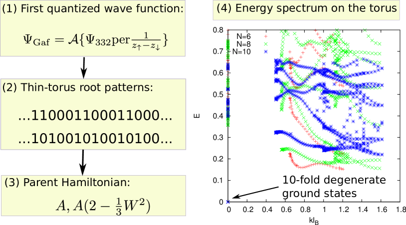
Figure 6: (Color online) Main steps in constructing the fermionic Gaffnian parent Hamiltonian. (i) Assume the first quantized wave function, in this example given by Eq. 40. (ii) Find the corresponding thin torus root patterns (here $1100011000...$ and $1010010100...$). (iii) Construct the parent Hamiltonian by consulting Eq. (26) and Table 3. (iv) Verify the construction and compute properties by exact diagonalization. Here, this is performed on a hexagonal torus with $N=6,8,10$ particles, finding a 10-fold ground state with exactly zero energy. The energy scale is set by $\gamma=1$ in Eq. 43. As the torus is stretched along one direction, the ground states evolve to the expected patterns $1100011000...$ and $1010010100...$. In addition, we obtain the entire low-lying neutral excitation spectrum, allowing one, in principle, to extract many other properties of the system.

V.1.2 Pfaffians and Haffnians

We next consider the generalized non-Abelian Pfaffian state at $1/q$ filling Moore and Read (1991); Read and Rezayi (1996). The wave function in the disk geometry reads

$$\text{Pf}\left(\frac{1}{z_{i}-z_{j}}\right)\prod_{i<j}(z_{i}-z_{j})^{q},$$ (46)

where even (odd) $q$ corresponds to a fermionic (bosonic) state. The Pfaffian is defined as

$${\rm Pf}(A)=\frac{1}{2^{n/2}(n/2)!}\sum_{\sigma\in S_{n}}\operatorname{sgn}(\sigma)\prod_{i=1}^{n/2}A_{\sigma(2i-1),\sigma(2i)},$$

where $A$ is the $n\times n$ skew-symmetric matrix $A_{ij}=1/(z_{i}-z_{j})$ for $n$ even. The case $q=2$ reduces to the familiar Moore-Read state, which is the ground state of purely 3-body interaction $U_{3}^{3}$. One would naively expect that $q>2$ states can be obtained by adding 2-body terms to $U_{3}^{3}$, but as one can explicitly verify, this is not the case.

By a power counting procedure Read and Rezayi (1996) (further elaborated on in Appendix C), the root configuration of the $1/q$-Pfaffian state is given by

$$10^{q-2}10^{q}10^{q-2}10^{q}......10^{q-2}10^{q}...$$ (47)

where $0^{q}$ represents a string of $q$ zeros. It follows that its parent Hamiltonian is given by the 3-body PP

$$U^{3}_{m=3(q-1)},$$ (48)

as well as all nonzero spinless 2-body PPs

$$U^{2}_{m<q-2}.$$ (49)

For the more interesting $q=4$ case which we have studied numerically, we require the two-body $U^{2}_{1}$ PP and three-body $U^{3}_{9,(i)}$ and $U^{3}_{9,(ii)}$ PPs given by Eq. 26 and Table 3. (Again, we emphasize that $U$’s promoted to how they appear in the Hamiltonian should be understood as polynomial amplitudes that enter the definition of operators $b_{n}^{\dagger},b_{n}$ in Eq. 10.)

Note that labels $(i),(ii)$ stand for two linearly independent 3-body PPs that occur for $m=9$. Thus, the 1/4 Pfaffian state is an example whose parent Hamiltonian contains a degenerate subspace of PPs. The state can alternatively be obtained numerically through Jack polynomials Bernevig and Regnault (2009) and the root configuration given above. We have confirmed that the overlap between the ground state of the parent Hamiltonian and the Jack polynomial wave function is equal to one (within machine precision) for $q=4$ and $N=6,8$ electrons. Note that experiments Luhman et al. (2008) find some evidence for an incompressible, potentially non-Abelian, $\nu=1/4$ state. This may be attributed to the Pfaffian $1/4$ state, although theoretical calculations suggest that the Halperin 553 state is also a candidate Papić et al. (2009).

For our final spin-polarized example we consider the fermionic Haffnian state Green (2001), whose bosonic counterpart was recently considered in Ref. Papić, 2014. The fermionic Haffnian occurs at the filling fraction $\nu=1/3$, and, up to COM translation, has the following root patterns Hermanns et al. (2011) on the torus: $110000110000...$ and $100100100100...$. The latter pattern is identical to that of the Laughlin state. The fermionic Haffnian vanishes as power $7$ as three particles are brought together, hence we need to impose an energy penalty for $m=6$ too, and the parent Hamiltonian consists of

$$U^{3}_{3},\;U^{3}_{5},\;{\rm and}\;U^{3}_{6},$$ (50)

which are given by Eq. 26 and Table 3.

V.2 Spinful states

We have previously mentioned that if we allow the spin degree of freedom to enter, the number of possible states obviously becomes much richer with interactions involving three or more particles. A systematic investigation of these states is left for future work. Here we content ourselves with illustrating our method by formulating parent Hamiltonians for several states that have been the subject of recent attention: the Spinful Gaffnian Davenport et al. (2013) and the non-Abelian Spin Singlet (NASS) states Ardonne et al. (2001). The Hamiltonians for these states have previously been written down for the sphere (or disk) geometry, which we now extend to the cylinder and torus. Furthermore, we propose the parent Hamiltonian for a certain type of state involving the permanent (“221 times permanent” state Ardonne and Regnault (2011)), for which the Hamiltonian was previously unknown.

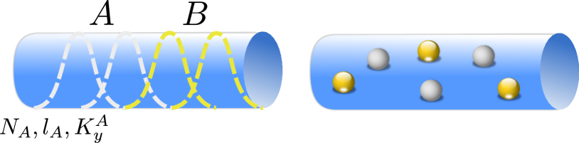
Figure 7: (Color online) Two choices of partitioning the system for computing the entanglement spectrum. Orbital cut (left) amounts to partitioning the system into two groups of orbitals $A$ and $B$, and tracing out the orbitals in $B$ (marked yellow). The Schmidt levels of $A$ can be classified by the number of particles $N_{A}$, the number of orbitals $l_{A}$, and the total momentum $K_{y}^{A}$. An alternative choice is particle partitioning (right), where some particles (marked in yellow) are traced out, regardless of their position.

In addition to formulating the parent Hamiltonians, we also computed the orbital (OES) and particle entanglement spectra (PES) for the respective states. Fig. 7 illustrates the two types of partitioning in the case of an open cylinder. After performing the cut, the entanglement spectrum can still have some remaining symmetry which can be used to classify the Schmidt levels. For example, for the OES, the total number of particles $N_{A}$ and the total number of orbitals $l_{A}$ in the left subsystem remain good quantum numbers. On the other hand, for the PES, the translation or rotation symmetry of the full system is preserved. For an open cylinder, as in Fig. 7, this means that the total momentum $K_{y}^{A}$ of the left subsystem is also a good quantum number:

$$K_{y}^{A}=\sum_{m\in A}m\hat{n}_{m},$$ (51)

with $\hat{n}_{m}$ the density operator acting on the momentum orbital $m$. This linear momentum on the cylinder corresponds to the $L_{z}$ projection of angular momentum on the sphere. The PES on the sphere, however, is also invariant under full SU(2) rotation, i.e. it forms multiplets of $L^{2}$. This symmetry is absent on a cylinder, where we can only use $K_{y}^{A}$ to classify the levels of the entanglement spectrum. This is discussed in more detail in the example in Sec. V.2.1. As we perform an orbital partition, the symmetry of the subsystem is reduced, and even on the sphere, the only remaining quantum number is $L_{z}$. Thus, the OES on the sphere can be directly compared with the OES on the open cylinder. Finally, for spinful states, the spin quantum number commutes with the reduced density operator of the OES, and thus allows for additional resolution of the ES level counting Thomale et al. (2011).

V.2.1 Spin-singlet Gaffnian state

Figure 8: (Color online) PES of the spin-singlet Gaffnian state for $N=12$ particles and $N_{\phi}=12$ flux quanta on an open cylinder with aspect ratio equal to 1. The spectrum is obtained by tracing out $N_{B}=N_{A}=6$ particles and plotted as a function of momentum $K_{y}^{A}$ in part A. Different values of $S_{z}^{A}$, the total $z$ component of spin in part $A$, are indicated in the inset.

The spin-singlet Gaffnian state is a nontrivial spinful generalization of the bosonic spin-polarized Gaffnian state by Davenport et al.Davenport et al. (2013). In addition to the two spin polarized 3-body terms with $S=3/2$, its parent Hamiltonian also contains the shortest range ($m=1$) term with $S=1/2$. In total, this encompasses the PPs

$$U^{3}_{0,S=3/2},\;U^{3}_{2,S=3/2}\;{\rm and}\;U^{3}_{1,S=1/2}.$$ (52)

As such, the spin-singlet Gaffnian wave function vanishes as the third power in the $S=3/2$ channel, and the second power in $S=1/2$. These projectors are given by Eqs. 26, 35 and Table 3 for $U^{3}_{0,3/2}$ and $U^{3}_{2,3/2}$, and Eq. LABEL:b1S12 for $U^{3}_{1,S=1/2}$ (with both spin orientations $\left|\uparrow\right\rangle\leftrightarrow\left|\downarrow\right\rangle$). In addition to these, we also add the total spin operator $S^{2}$ to our Hamiltonian, to ensure that the ground state is a spin-singlet.

By diagonalizing the Hamiltonian (52) numerically, we find a zero-energy ground state at filling factor $\nu=4/5$ and shift of $-3$ on a finite cylinder for $N=4,8,$ and $12$ particles. We have furthermore computed the PES Sterdyniak et al. (2011) for $N=12$ particles and $N_{\phi}=12$ flux quanta, shown in Fig. 8. As illustrated in Fig. 7 (right), to perform a PES “partition”, we divide the system into parts $A$ and $B$, which both contain $N_{\phi}$ orbitals, but $N_{A}$ and $N_{B}$ particles, respectively, such that $N_{A}+N_{B}=N$. To obtain Fig. 8, we have traced out $N_{B}=6$ particles from the system. The PES obtained in this way provides information about the counting of quasihole excitations of the given state, as shown in Ref. Sterdyniak et al., 2011.

We compare the counting in Fig. 8 with the corresponding PES obtained on the sphere in Davenport et al. Davenport et al. (2013). Note that our result in Fig. 8 superficially looks different from the result in Ref. Davenport et al., 2013. This is because the PES partition preserves the symmetry of the ground state, causing the PES on the sphere to have exact rotational symmetry which is absent for our open cylinder. In other words, on an open cylinder, the good quantum number after partitioning is only the linear momentum $K_{y}^{A}$. This quantum number, in turn, corresponds to the $L_{z}$ projection of angular momentum on the sphere. This, however, does not exhaust all symmtries of the PES on the sphere, where the full angular momentum $L^{2}$ is a good quantum number. This additional degeneracy of the PES is factored out in Ref. Davenport et al., 2013. Furthermore, on both the sphere and cylinder, due to the singlet property of the wave function, we expect the PES levels to be multiplets of the $S^{2}$ operator Thomale et al. (2011), as can be verified in Fig. 8. The most important universal information is the counting of PES levels per momentum sector, which we find to be in agreement with Ref. Davenport et al., 2013. As we restore the $L^{2}$ degeneracy in the PES given in Ref. Davenport et al., 2013, the counting for the first three sectors is a single level with $S=1$ and $L^{z}=22$, 4 levels at $L_{z}=21$ (two with $S=1$ and two with $S=0$), and 10 levels at $L_{z}=20$ (one of them with $S=2$, 6 with $S=1$ and 3 with $S=0$). While the finite-size splitting between these levels is non-universal (and differs between sphere and cylinder), we indeed obtain the identical counting per sector (Fig. 8).

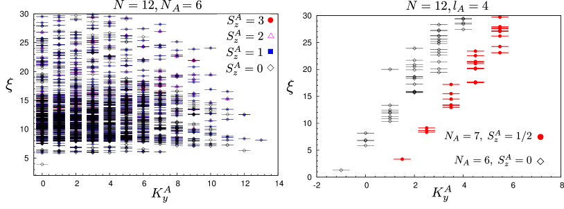
Figure 9: (Color Online) PES (left) and OES (right) for the NASS $\nu=4/3$ state. The system contains $N=12$ bosons on a finite cylinder with aspect ratio 1. For PES, the subsystem $A$ contains $N_{A}=6$ particles, and PES is plotted as a function of momentum $K_{y}^{A}$ of subsystem $A$. The states are labeled by different values of $S_{z}^{A}$, the total $z$ component of spin in part $A$, as indicated in the inset. For OES, the subsystem $A$ contains $l_{A}=4$ orbitals, where we show data for $N_{A}=6$ and $N_{A}=7$. The spectrum is resolved as a function of momentum $K_{y}^{A}$ of subsystem $A$.

V.2.2 The NASS state

Another class of non-Abelian spin-singlet states has been proposed by Ardonne et al.Ardonne et al. (2001) under the name “non-Abelian spin singlet” states (NASS). The bosonic family of such states occurs at filling factors $\nu=2k/3$. According to Ref. Ardonne and Regnault, 2011, the NASS wave function ought to vanish quadratically when we bring together $k+1$ particles of the same spin, and linearly for $k+1$ particles of different spins. For SU(2) spins, such wave functions only exist in the $[k+1]$ and $[k,1]$ representations. Its parent Hamiltonian should therefore contain the PPs $U^{k}_{m=0,S=k/2}$ and $U^{k}_{m=0,S=k/2-1}$, since the simplest nontrivial totally/partially symmetric polynomial are of degrees two and one, respectively. Explicitly, the $b_{n}^{m=0\dagger}$ operators are

$$b_{n,S=k/2}^{0\dagger}\left|0\right\rangle = e^{-\frac{\kappa^{2}}{2}\sum_{i}^{k}\bar{n}_{i}^{2}}\left|\uparrow\uparrow...\uparrow\right\rangle,$$ (53)

$$b_{n,S=k/2-1}^{0\dagger}\left|0\right\rangle = e^{-\frac{\kappa^{2}}{2}\sum_{i}^{k}\bar{n}_{i}^{2}}[\left|\uparrow\uparrow...\uparrow\downarrow\right\rangle+\left|\uparrow\uparrow...\downarrow\uparrow\right\rangle$$ (54)

$$+ \left|\uparrow\uparrow...\downarrow\uparrow\uparrow\right\rangle+...+\left|\downarrow\uparrow...\uparrow\right\rangle],$$

and similarly for the terms $S\rightarrow-S$ obtained by exchanging $\left|\uparrow\right\rangle\leftrightarrow\left|\downarrow\right\rangle$.

The simplest member $k=2$ of the NASS family has recently been studied from the “squeezing” perspective Ardonne and Regnault (2011). Below we complement these results by independently generating the NASS $k=2$ state using its parent Hamiltonian in Eqs. 53 and 54. We compute its PES and OES on a finite cylinder, Fig. 9. The PES and OES are computed for $N=12$ bosons on a cylinder with aspect ratio 1. Similar to the previous cases, the universal information in the PES spectrum – the counting of levels per momentum sector – is in agreement with the independently obtained data in Ref. Ardonne and Regnault, 2011 on the sphere. In this case, the bipartition of the system is obtained by fixing the cut such that there are $l_{A}=4$ orbitals in part A. We compute the OES for two choices of the total number of particles in A, $N_{A}=6$ and $N_{A}=7$. We see that the counting of the OES changes as a function of $N_{A}$, as it often happens for non-Abelian states where moving the cut probes different topological sectors of the theory, in this case associated with SU$(3)_{2}$ CFT.

V.2.3 Halperin-permanent states

Finally, we tackle more complex examples of non-Abelian states that involve a product of Halperin multicomponent states Halperin (1983) and the permanent. To be specific, we study states of the following form in the disk geometry:

$$\Phi_{lln} = \text{Per}\left(\frac{1}{z_{i}-w_{j}}\right)\psi_{lln}(\{z\},\{w\}),$$ (55)

where $z_{i},w_{i}$ refer to the spin up and spin down particle coordinates, respectively, and $\psi_{lln}$ is the Halperin wave function Halperin (1983), an example of which was given in Eq. 41 for $l=3$, $n=2$. We have suppressed, as usual, the spinor and Gaussian parts of the wave function. The permanent was defined in Eq. (42).

We are particularly interested in the states $\Phi_{111}$ and $\Phi_{221}$. The former was introduced by Moore and Read Moore and Read (1991), and subsequently analyzed in detail by Read and Rezayi Read and Rezayi (1996) (see also Ref. Green, 2001). As a prototypical example of a state that derives from a non-unitary CFT, it was shown to describe a critical point between the ferromagnet and paramagnet. Its thin-torus limit was recently studied in Ref. Papić, 2014. The latter state, $\Phi_{221}$, has been addressed by Ardonne and Regnault Ardonne and Regnault (2011), who computed some of its properties by identifying its root configuration on the sphere and deriving its “squeezing” properties. Here we show how to write down the parent Hamiltonian for these two states for the cylinder and torus geometry. This is of particular interest in the case of $\Phi_{221}$, where such a Hamiltonian has not been reported for any geometry before.

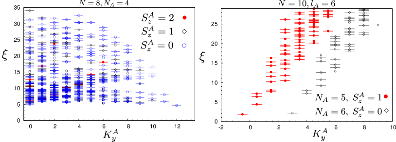
Figure 10: (Color online) PES (left) and OES (right) for the $\Psi_{221}$ state on a finite cylinder with aspect ratio equal to 1. For PES, we consider $N=8$ bosons and the subsystem $A$ contains $N_{A}=4$ particles. The PES is plotted as a function of momentum $K_{y}^{A}$ of subsystem $A$. Different values of $S_{z}^{A}$, the total $z$ component of spin in part $A$, are indicated in the inset. For OES, we consider $N=10$ bosons, the subsystem $A$ contains $l_{A}=6$ orbitals and the OES is plotted as a function of momentum $K_{y}^{A}$ of subsystem $A$, for two values of the total number of particles in subsystem $A$ ($N_{A}=5$ and $N_{A}=6$).

To begin with, we want to derive many-body projection Hamiltonians whose null space contains $\Phi_{lln}$. We first consider 2-body interactions. From Eq. 55, $\Phi_{lln}$ vanishes as the $l^{th}$ power when $z_{i}\rightarrow z_{j}$ (or $w_{i}\rightarrow w_{j}$). Hence we need 2-body terms $U^{2}_{m,S=1}$ where $m<l$ and $|S|=1$, i.e. in the $\left|\uparrow\uparrow\right\rangle$ or $\left|\downarrow\downarrow\right\rangle$ channels. In the $S=0$ (or $\left|\uparrow\downarrow\right\rangle$) channel, however, one term in the permanent will cause $\Phi_{lln}$ not to vanish for $z_{i}\rightarrow w_{k}$. Hence we do not need any $U^{2}_{m,S=0}$.

For 3-body interactions, we find that the Halperin function parts contribute a degree of $l+2n$ for $S=\frac{1}{2}$ (or the $\left|\uparrow\uparrow\downarrow\right\rangle$, $\left|\uparrow\downarrow\downarrow\right\rangle$, etc.) channels. Also, the permanent will remove one degree. Hence we need $U^{3}_{m,1/2}$ for $m<l+2n-1$. An analogous analysis for $\left|\uparrow\uparrow\uparrow\right\rangle$ or $\left|\downarrow\downarrow\downarrow\right\rangle$ reveals that we also need $U^{3}_{m,3/2}$ for $m<3l$. The matter simplifies a bit since not all of the requisite $U^{2,3}_{m,S}$ mentioned above actually exist. In Sec. IV and also Table 1 of Ref. Davenport and Simon, 2012, the PPs $U^{2}_{m,S}$ are nonzero for even $m$ when $l$ is even and $S=1$, or $l$ odd and $S=0$ (and vice versa for total anti-symmetry in spin-orbit space). For $N=3$, $U^{3}_{m,1/2}$ exists for $m\geq 1$, but $U^{3}_{m,3/2}$ does not exist for $m=0,1,2$ in the case of fermions (odd $l$). In summary, the above considerations for $n=1$ and $l=1,2$ imply that only $U^{3}_{1,1/2}$ is required to produce $\Phi_{111}$, consistent with Ref. Read and Rezayi, 1996. On the other hand, $U^{2}_{0,1}$, $U^{3}_{1,1/2}$, $U^{3}_{2,1/2}$, and $U^{3}_{m,3/2}$ for $m=0,2,3,4,5$ are all required to produce $\Phi_{221}$. Therefore, we see that formulating the parent Hamiltonian for $\Phi_{221}$ is indeed rather involved, and crucially benefits from the systematic approach we follow here.

For completeness, we quote the explicit expressions for these two Hamiltonians in the form $U^{N}_{m,S}=\sum_{n}b_{n}^{m,S\dagger}b_{n}^{m,S}+(\left|\uparrow\right\rangle\leftrightarrow\left|\downarrow\right\rangle)$. For the $\Phi_{111}$ state, we have

$$H_{111} = U^{3}_{1,1/2}\propto\sum_{n}b^{1,1/2\dagger}_{n}b^{1,1/2}_{n},$$ (56)

with the corresponding operator and polynomial amplitude

$$b^{1,1/2}_{n} = \kappa^{3/2}\sum_{\sum n_{i}=n}p_{1,1/2}(\kappa;\{n\})e^{-\frac{\kappa^{2}}{3}W^{2}}c_{n_{1}}c_{n_{2}}c_{n_{3}},$$

$$p_{1,1/2} = (\bar{n}_{1}-\bar{n}_{2})\left|\uparrow\uparrow\downarrow\right\rangle+(\bar{n}_{2}-\bar{n}_{3})\left|\downarrow\uparrow\uparrow\right\rangle$$ (58)

$$+ (\bar{n}_{3}-\bar{n}_{1})\left|\uparrow\downarrow\uparrow\right\rangle,$$

where as before $\bar{n}_{i}=n_{i}-\frac{1}{3}\sum_{j}n_{j}$. For $\Phi_{221}$, we have

$$H_{221} = U^{2}_{0,1}+\sum_{m=1,2}\gamma_{m}U^{3}_{m,1/2}$$ (59)

$$+ \sum_{m=0,2,3,4,5}\eta_{m}U^{3}_{m,3/2},$$

where again $\gamma_{m}$ and $\eta_{m}$ can be chosen to be arbitrary positive constants.

We have numerically diagonalized the Hamiltonian (59) and verified that it gives a unique zero energy ground state on finite cylinders when $N_{\phi}=3N/2-3$. By stretching the cylinder, we confirmed that the ground state reduces to the pattern $(\uparrow,\downarrow)00(\uparrow,\downarrow)00...$, which coincides with the root configuration given in Ref. Ardonne and Regnault, 2011. In Fig. 10 (left) we compute the PES for $N=8$ bosons, which can be directly compared with Fig. 7 in Ref. Ardonne and Regnault, 2011. As expected, we find an agreement in the counting of the PES levels between our results on the cylinder and the sphere data in Ref. Ardonne and Regnault, 2011. Finally, we also provide a plot of the OES in Fig. 10 (right). As shown by Li and Haldane Li and Haldane (2008), a non-Abelian state like the Moore-Read state will have different counting depending on the position of the orbital entanglement cut, which effectively probes different topological sectors of the theory. This is also the case in our example, as we see the counting changes depending on the number of particles in subsystem $A$ while the location of the cut remains fixed. Furthermore, the spectrum is fully chiral, which suggests that this state may be described by a simple CFT as conjectured in Ref. Ardonne and Regnault, 2011. The CFT can in principle be identified using the counting of the OES in Fig. 10. For this purpose, larger systems may be required in order to verify that the counting we see in Fig. 10 is saturated and indeed corresponds to the thermodynamic limit, which we defer to future work.

VI Conclusion

We have provided a general method for constructing quantum Hall parent Hamiltonians with the desired type of clustering properties on cylinder and torus geometries. The approach developed here completes the program initiated in Ref. Simon et al., 2007a which is suited for the disk and sphere geometry that have a conserved $z$-component of angular momentum. We have performed extensive analytic and numerical checks of the proposed model Hamiltonians, and generally find complete agreement with previous results if available. We have also demonstrated that it is possible to construct the parent Hamiltonians for some rather complex spinful non-Abelian states which previously have not been provided in the literature.

The method presented here opens up several future directions. One can use the Hamiltonians derived here to systematically scan for filling factors where the Hamiltonians have zero-energy ground states, in the spirit of Ref. Simon et al., 2010. Performing this kind of search is much more natural in the torus geometry which does not suffer from the known shift bias Wen and Zee (1992). Furthermore, our approach straightforwardly generalizes to 4-body interactions whose possible incompressible ground states have not been systematically investigated before. Another interesting extension to pursue is the study of multicomponent states beyond the familiar SU(2) spin, such as the SU(4) valley/spin symmetric non-Abelian states. They may have relevance in the realization of FQHE in graphene, where the open accessibility of the electron gas may allow for further tunability of the interaction profile Dean et al. (2011); Papić et al. (2011).

Appendix A Barycentric coordinates for many-body pseudopotentials

We describe how to find a manifestly $S_{N}$-symmetric embedding of the tuple $(\bar{n}_{1},...,\bar{n}_{N})$ onto the $(N-1)$-dimensional simplex in $\mathbb{R}^{N-1}$. This can be achieved in barycentric coordinates, which is also useful for diverse applications involving permutation symmetry with a linear constraint Lee and Lucas (2014). The most straightforward construction is to write

$$\vec{x}=\kappa\sum_{k=1}^{N}\bar{n}_{k}\vec{\beta}_{k},$$ (60)

where $\vec{x}\in\mathbb{R}^{N-1}$ and $\{\vec{\beta}_{k}\}$, $k=1,...,N$ forms a linearly dependent set of basis vectors, also in $\mathbb{R}^{N-1}$, normalized so that

$$\vec{\beta}_{j}\cdot\vec{\beta}_{k}=\frac{N}{N-1}\delta_{jk}-\frac{1}{N-1}.$$ (61)

Geometrically, the $\beta_{k}$’s define the vertices of a simplex, and are at angle of $\cos^{-1}(-1/(N-1))$ from one another. The vertex $k$ corresponds to the least isotropic configuration with $\bar{n}_{k}\propto\frac{N-1}{N}$ and $\bar{n}_{j}\propto-\frac{1}{N}$, $j\neq k$. A basis consistent with the above requirements is

$$\vec{\beta}_{1} =(1,0,\ldots,0),$$ (62a)

$$\vec{\beta}_{2} =(C_{1},S_{1},\ldots,0),$$ (62b)

$$\vec{\beta}_{3} =(C_{1},S_{1}C_{2},S_{1}S_{2},\ldots,0),$$ (62c)

$$\vec{\beta}_{4} =(C_{1},S_{1}C_{2},S_{1}S_{2}C_{3},S_{1}S_{2}S_{3},\ldots,0),$$ (62d)

$$\vdots$$

$$\vec{\beta}_{N-1} =(C_{1},S_{1}C_{2},S_{1}S_{2}C_{3},\ldots,S_{1}\cdots S_{N-2}),$$ (62e)

$$\vec{\beta}_{N} =(C_{1},S_{1}C_{2},S_{1}S_{2}C_{3},\ldots,-S_{1}\cdots S_{N-2}),$$ (62f)

with $S^{2}_{k}+C^{2}_{k}=1$, $1\leq k\leq N-2$. Upon enforcing the scalar product constraint in Eq. 61, we require that $S_{k+1}=1-(1+1/N)/(\prod_{j=1}^{k}S_{k})^{2})$, which also implies that $C_{k}^{2}+S_{k}^{2}C_{k+1}=C_{k}$. A simple solution fortunately exists:

$$C_{k}=-\frac{1}{N-k},$$ (63)

which implies that the $k$-th projected component of the relative angles between the position vectors of the vertices approaches $\pi$ as $k$ and $N$ increase. We proceed by substituting Eq. 63 into the explicit form of vertex positions $\vec{\beta}_{k}$, and expressing the latter in terms of the spherical coordinates. From Eq. 60, we can easily check

$$\bar{n}_{k}=\frac{N-1}{N\kappa}\vec{x}\cdot\vec{\beta}_{k},$$ (64)

and that

$$W^{2}=|\vec{x}|^{2}=\frac{N\kappa^{2}}{N-1}\sum_{k}^{N}\left(n_{k}-\frac{n}{N}\right)^{2}=\frac{N\kappa^{2}}{N-1}\sum_{k}^{N}\bar{n}_{k}^{2}.$$ (65)

For the purpose of orthogonalizing the PPs over the inner product measure in Eq. 14, we will also need to express $\vec{x}$ explicitly in terms of angles in origin-centered spherical coordinates:

$$x_{1} =W\cos\varphi_{1},$$ (66a)

$$x_{2} =W\sin\varphi_{1}\cos\varphi_{2},$$ (66b)

$$\vdots$$

$$x_{N-2} =W\cos\varphi_{k}\prod_{k=1}^{N-3}\sin\varphi_{k},$$ (66c)

$$x_{N-1} =W\prod_{k=1}^{N-2}\sin\varphi_{k}.$$ (66d)

Substituting the explicit expressions from Eqs. 62 and 66 into Eq. 64, we obtain

$$\bar{n}_{1} =\frac{N-1}{N\kappa}W\cos\varphi_{1},$$ (67)

$$\bar{n}_{2} =\frac{W}{N\kappa}\left(-\cos\varphi_{1}+\sqrt{N(N-2)}\sin\varphi_{1}\cos\varphi_{2}\right),$$ (68)

$$\bar{n}_{k} =\frac{W}{N\kappa}[-\cos\varphi_{1}-\sqrt{\frac{N}{N-2}}\sin\varphi_{1}\cos\varphi_{2}$$

$$\;\;\;\;\;-\sum_{j=2}^{k-2}\sqrt{\frac{N!}{(N-j-2)!}}\frac{\left(\prod_{i=1}^{j}\sin\varphi_{i}\right)\cos\varphi_{j+1}}{(N-j)(N-j-1)}$$

$$\;\;\;\;\;+\sqrt{\frac{N!}{(N-k-1)!}}\frac{\left(\prod_{i=1}^{k-1}\sin\varphi_{i}\right)\cos\varphi_{k}}{N-k+1}],$$ (69)

$$\vdots$$

$$\bar{n}_{N-1} =\frac{W}{N\kappa}[-\cos\varphi_{1}-\sqrt{\frac{N}{N-2}}\sin\varphi_{1}\cos\varphi_{2}$$

$$\;\;\;\;\;-\sum_{j=2}^{N-3}\sqrt{\frac{N!}{(N-j-2)!}}\frac{\left(\prod_{i=1}^{j}\sin\varphi_{i}\right)\cos\varphi_{j+1}}{(N-j)(N-j-1)}$$

$$\;\;\;\;\;+\frac{\sqrt{N!}}{2}\left(\prod_{i=1}^{N-2}\sin\varphi_{i}\right)],$$ (70)

$$\bar{n}_{N} =\frac{W}{N\kappa}[-\cos\varphi_{1}-\sqrt{\frac{N}{N-2}}\sin\varphi_{1}\cos\varphi_{2}$$

$$\;\;\;\;\;-\sum_{j=2}^{N-3}\sqrt{\frac{N!}{(N-j-2)!}}\frac{\left(\prod_{i=1}^{j}\sin\varphi_{i}\right)\cos\varphi_{j+1}}{(N-j)(N-j-1)}$$

$$\;\;\;\;\;-\frac{\sqrt{N!}}{2}\left(\prod_{i=1}^{N-2}\sin\varphi_{i}\right)].$$ (71)

These are the explicit expressions for transcribing the $\bar{n}_{j}$, $1\leq j\leq N$ indices directly into spherical coordinates. In (69), $k$ ranges from $3$ to $N-2$.

Appendix B Second-quantized pseudopotentials vs. real-space projection Hamiltonians

We provide a brief comparison between the second-quantized PPs that have been derived in this paper and real-space projection Hamiltonians elsewhere in the literature, e.g. Trugman-Kivelson type Hamiltonians on the infinite plane. We show that our geometric PP construction avoids certain ambiguities that plague the latter approaches.

Neglecting internal DOFs for simplicity, a generic real-space PP living in total relative angular momentum sectors up to $m$ takes the form

$$H(\vec{r}_{1},...,\vec{r}_{N})=\left(\prod^{N}_{j=1}\nabla_{j}^{2d_{j}}\right)\delta^{2}(\vec{r}_{1}-\vec{r}_{2})...\delta^{2}(\vec{r}_{N-1}-\vec{r}_{N})$$ (72)

such that $\sum_{j}d_{j}=m$. The various $d_{j}$’s refer to how the derivatives are distributed among the particles. In this form, there is no simple one-to-one correspondence between the $d_{j}$ values and the relative weight of $H$ in the various $m$ sectors. To find the relative weights, one has to project $H$ onto the sector spanned by a state with angular momentum $m$. It is most convenient to adopt the symmetric gauge, where such a state takes the form $\left|\Psi_{m}\right\rangle\propto p(\tilde{z}_{1},...,\tilde{z}_{N})e^{-\frac{1}{4}\sum_{j}|z_{j}|^{2}}|z_{1},...,z_{N}\rangle$ where $p$ is a symmetric or antisymmetric polynomial and $z_{j}=x_{j}+iy_{j}$ refers to the particle position ($\tilde{z}$ defined below):

$$\langle\Psi_{m}|H\left|\Psi_{m}\right\rangle=$$

$$\left(\prod_{j=1}^{N}\int d^{2}\vec{r}_{j}\right)\Psi_{m}^{*}(\vec{r}_{1},...,\vec{r}_{N})H(\vec{r}_{1},...,\vec{r}_{N})\Psi_{m}(\vec{r}_{1},...,\vec{r}_{N}).$$

Upon substituting $\Psi_{m}$ and integrating by parts, we can express $\langle\Psi_{m}|H|\Psi_{m}\rangle$ as

$$\langle\Psi_{m}|H\left|\Psi_{m}\right\rangle=$$ (74)

$$\left(\prod_{j=1}^{N}\int d^{2}\vec{r}_{j}\right)\delta^{2}(\vec{r}_{1}-\vec{r}_{2})...\delta^{2}(\vec{r}_{N-1}-\vec{r}_{N})$$

$$\times \left(\prod^{N}_{j=1}\nabla_{j}^{2d_{j}}\right)[\Psi_{m}^{*}(\vec{r}_{1},...,\vec{r}_{N})\Psi_{m}(\vec{r}_{1},...,\vec{r}_{N})],$$

which can be evaluated as

$$\langle\Psi_{m}|H\left|\Psi_{m}\right\rangle=$$

$$= 4^{m}\left(\prod_{j=1}^{N}\int dz_{j}dz^{*}_{j}\right)\delta^{2}(z_{1}-z_{2})...\delta^{2}(z_{N-1}-z_{N})$$

$$\left(\prod^{N}_{j=1}\partial_{z^{*}_{j}}^{2d_{j}}\Psi_{m}^{*}(z_{1}^{*},...,z_{N}^{*})\right)\left(\prod^{N}_{j=1}\partial_{z_{j}}^{2d_{j}}\Psi_{m}(z_{,}...,z_{N})\right),$$

where $\nabla^{2}=4\partial_{z}\partial_{\bar{z}}$ has been used. The delta functions, which enforce that all $z_{j}$ be equal, also enforce $\tilde{z}_{j}=z_{j}-\frac{1}{N}\sum_{j}z_{j}=0\;\forall\;j$. Thus we only get a nonzero contribution from constant integrands. Specific examples were worked out in the appendices of Ref. Simon et al., 2007b; in general, an operator $H$ has an overlap with various $m$ sectors, and a PP that lies purely in one $m$ sector must be a complicated linear combination of the Trugman-Kivelson terms with various sets of $d_{j}$’s. Some progress was made in Ref. Lee et al., 2013, where operators containing $L_{m}\left(\frac{N\kappa^{2}}{2(N-1)\nabla_{1}^{2}}\right)$ were shown to be contained purely in one $m$ sector. That, however, does not always work for fermions as will be explained below.

The mathematical complications above are further aggravated when the space of PPs in the sector $m$ is degenerate. In particular, the matrix $\langle\Psi_{ma}|H\left|\Psi_{mb}\right\rangle$ is not of full rank and some combinations of bona-fide PPs of degree $m$ will still not give a positive energy penalty to states in the $m$ sector Simon et al. (2007b). In particular, it is possible for certain Trugman-Kivelson Hamiltonians with $2m$ derivatives to evaluate to zero upon taking into account the fermionic antisymmetry. Consider for instance the $N=3$ fermionic state $\left|\Psi_{3}\right\rangle\propto(\tilde{z}_{1}-\tilde{z}_{2})(\tilde{z}_{2}-\tilde{z}_{3})(\tilde{z}_{3}-\tilde{z}_{1})|z_{1},z_{2},z_{3}\rangle$. The following operators have a zero projection on it:

$$\langle\Psi_{3}|\nabla^{6}_{j}\delta^{2}(r_{1}-r_{2})\delta^{2}(r_{2}-r_{3})|\Psi_{3}\rangle=0$$

and

$$\langle\Psi_{3}|\nabla^{2}_{1}\nabla^{2}_{2}\nabla^{2}_{3}\delta^{2}(r_{1}-r_{2})\delta^{2}(r_{2}-r_{3})|\Psi_{3}\rangle=0.$$

Indeed, the only nonvanishing Trugman-Kivelson type fermionic PP in the $U^{N=3}_{m=3}$ sector is $H=\nabla^{4}_{i}\nabla^{2}_{j}\delta^{2}(r_{1}-r_{2})\delta^{2}(r_{2}-r_{3})$. As $|\Psi_{3}\rangle$ is of degree $\leq 2$ in each variable, $H$ must contain a derivative of degrees $2d_{j}\leq 4$ in each variable for a nonzero projection. Since only constant terms in the integrand of Eq. LABEL:realproject contribute, we also need derivatives in all three particle coordinates.

By contrast, our PP construction appeals to the orthogonality structure of the PPs from the outset, and avoids all of the above problems that generically arise when one attempts to use the Trugman-Kivelson approach in more complicated many-body cases.

Appendix C Pseudopotential parent Hamiltonian from a given wave function

We briefly summarize the heuristic procedure how to determine the PPs whose null spaces contain a given QH state. These are the PPs that should be included in its parent Hamiltonian, since they penalize denser or “simpler” states that will otherwise be realized at the same filling fraction. The method consists of two steps: (i) identify the thin-torus root pattern from the first-quantized wave function (Sec. C.1), and (ii) use the root pattern and power counting to obtain the PPs (Sec. C.2).

C.1 Wave function to root pattern

Suppose we are given a QH wave function with the polynomial part $\psi(z_{1},z_{2},...)$, where the $z_{i}$’s denote the positions of particles. In the infinite plane, $z_{j}$ is the usual complex coordinate $z_{j}=x_{j}+iy_{j}$. Since we will work on a cylinder geometry, however, we need to perform a stereographic mapping: $z_{j}\to e^{\kappa z_{j}}$, where $\kappa=2\pi/L_{y}$ is shown in Fig. 11. For simplicity, assume there are no internal degrees of freedom.

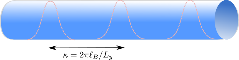
Figure 11: (Color online) In the limit of thin cylinder ($\kappa\to\infty$), the single-particle orbitals become well-separated from one another. As a consequence, the dominant configurations (“root patterns”) in the expansion of a many-body state $\Psi$ are those Fock states where particles minimize their classical electrostatic energy.

To each wave function defined on a cylinder, we can assign one or several thin-cylinder root patterns. Those are the Fock states with non-zero weight as the circumference of the cylinder is taken to zero ($\kappa\to\infty$). Typically, any given FQH state $\left|\psi\right\rangle$ in the thermodynamic limit decomposes onto many Fock states, as $\left|\psi\right\rangle$ represents a strongly correlated state. However, when the cylinder is stretched, the weights of most of the Fock states in the decomposition vanish. The only Fock states surviving in the limit $\kappa\to\infty$ are called “root patterns” and are useful for finding the parent Hamiltonian (Laplacian) for $\left|\psi\right\rangle$ as its kernel.

In order to find the root pattern, we must examine the dominant terms in the decomposition of $\psi$ as $\kappa\to\infty$. Usually, this amounts to solving a classical electrostatic problem. Here, we consider the case of an open cylinder, where the root pattern will typically be unique. To get the remaining root patterns, that arise due to topological degeneracy or non-Abelian statistics, one must consider the system on a torus. Due to the complicated form of torus wave functions, it is more convenient to work on a cylinder but perform a flux insertion which allows one to access other topological sectors. Details of this are given e.g. in Ref. Seidel and Yang, 2008.

Fixing the total number of particles, we study the dominating term in $\psi$. It is $z_{1}^{m_{1}}z_{2}^{m_{2}}z_{3}^{m_{3}}...$ such that no other term (denoted by ^′) has $m^{\prime}_{1}>m_{1}$ or, $m^{\prime}_{2}>m_{2}$ if $m^{\prime}_{1}=m_{1}$ or, $m^{\prime}_{3}>m_{3}$ if $m^{\prime}_{1}=m_{1}$ and $m^{\prime}_{2}=m_{2}$, etc. The root pattern can then be written down as the partition defined by $m_{1},m_{2},...$:

$$(m_{1},m_{2},m_{3},...)\rightarrow 10...010...01...$$ (76)

where the $1$’s are at position $m_{1},m_{2},...$. If two $m_{i}$’s coincide, as can occur for bosons or multicomponent fermions, we shall label that position by ’$2$’ and so forth. For instance, consider the $1/m$ Laughlin state with $2$ particles. We have $\psi(z_{1},z_{2})=(z_{1}-z_{2})^{m}$ which, when expanded out, contains monomials

$$\{z_{1}^{m},z_{1}^{m-1}z_{2},z_{1}^{m-2}z_{2}^{2},...\}$$ (77)

Evidently, the term $z_{1}^{m}z_{2}^{0}$ is in the root pattern. Had we considered a droplet of $N$ particles, this term would have become $z_{1}^{m(N-1)}z_{2}^{m(N-2)}...z_{N-1}^{m}z_{N}^{0}$, with total degree $\frac{mN(n-1)}{2}$ and the root

$$10^{m-1}10^{m-1}1...,$$ (78)

where $0^{m-1}$ represents a string of $m-1$ consecutive zeroes. For this simplest case, a droplet of $N=2$ particles is sufficient to determine the root configuration. Because we deal with translationally invariant states, a root configuration for larger $N$ is obtained by repeating the minimal pattern.

Let us now consider a more complicated example such as the generalized Pfaffian state introduced in Eq. (46) in Sec. V. By using the identity $[Pf(A)]^{2}=Det(A)$, one can show by induction starting from $n=4$, the most compact particle droplet, that the dominating term is $z_{1}^{3q-1}z_{2}^{2q}z_{3}^{q-1}$. This defines the root configuration in Eq. (47), $10^{q-2}10^{q}10^{q-2}10^{q}...$. It is also easy to read off the filling fraction from the above: we have $2$ particles per period, and each period has length $2q$. Hence the filling fraction is $\frac{2}{2q}=1/q$.

C.2 Root pattern to parent Hamiltonian

Given a root pattern, we can easily infer what relative angular momentum states should be penalized to construct a projector onto the state. For instance, if the closest pair of particles are $...10^{l}1...$, no two particles have relative angular momentum less than $l+1$. Hence the state should lie in the null space of any two-body PPs with $U^{2}_{m}$, $m\leq l$. Consequently, the parent Hamiltonian should be a linear combination of these PPs, so that it penalizes all states denser than the given one. This is discussed at length in Ref. Simon et al., 2007a.

To figure out the required many-body PPs, we apply the above procedure analogously to clusters of particles with minimal relative angular momentum. Note that some many-body PPs need not be included if the interaction is already precluded by particle (anti)symmetry: Consider the $1/q$ Pfaffian state described above, with a root given by Eq. 47. Obviously, no two particles have relative angular momentum less than $q-1$. Naively, we will then need to include all $U^{2}_{m}$ with $m\leq q-2$. The $1/q$ Pfaffian state, however, is fermionic (bosonic) when $q$ is even(odd), and $U^{2}_{q-2}$ exactly vanishes in both cases. Hence the parent Hamiltonian only contains $U^{2}_{m<q-2}$.

Let us finally analyze 3-body interactions. From the root pattern, the minimal total relative angular momentum is $l=(q-1)+2q=3q-1$. However, configurations with $l=3q-2=2(q-1)+q$ automatically vanish since they require pairs of particles with relative angular momenta $q$ and $q-1$ simultaneously, which are forbidden by either fermionic or bosonic statistics. With lower 3-body relative angular momentum already excluded by the 2-body PPs, the only 3-body PP we need to include in the parent Hamiltonian is $U^{3}_{3q-3}$. As the root pattern repeats from the third particle, there is no need to consider interactions with $4$ or more bodies.

References

- Tsui et al. (1982) D. C. Tsui, H. L. Stormer, and A. C. Gossard, “Two-dimensional magnetotransport in the extreme quantum limit,” Phys. Rev. Lett. 48, 1559–1562 (1982).
- Laughlin (1983) R. B. Laughlin, “Anomalous quantum hall effect: An incompressible quantum fluid with fractionally charged excitations,” Phys. Rev. Lett. 50, 1395–1398 (1983).
- Haldane (1983) F Duncan M Haldane, “Fractional quantization of the hall effect-a hierarchy of incompressible quantum fluid states,” Physical Review Letters 51, 605–608 (1983).
- Haldane (1990) F. D. M. Haldane, The Quantum Hall Effect, edited by R. E. Prange and S. M. Girvin (Springer, New York, 1990).
- Fano et al. (1986) G. Fano, F. Ortolani, and E. Colombo, “Configuration-interaction calculations on the fractional quantum hall effect,” Phys. Rev. B 34, 2670–2680 (1986).
- Nayak et al. (2008) Chetan Nayak, Steven H. Simon, Ady Stern, Michael Freedman, and Sankar Das Sarma, “Non-abelian anyons and topological quantum computation,” Rev. Mod. Phys. 80, 1083–1159 (2008).
- Pachos (2012) J.K. Pachos, Introduction to Topological Quantum Computation, Introduction to Topological Quantum Computation (Cambridge University Press, 2012).
- Moore and Read (1991) Gregory Moore and Nicholas Read, “Nonabelions in the fractional quantum hall effect,” Nuclear Physics B 360, 362 – 396 (1991).
- Greiter et al. (1991) Martin Greiter, Xiao-Gang Wen, and Frank Wilczek, “Paired hall state at half filling,” Physical review letters 66, 3205 (1991).
- Greiter et al. (1992) Martin Greiter, XG Wen, and Frank Wilczek, “Paired hall states,” Nuclear Physics B 374, 567–614 (1992).
- Read and Rezayi (1996) N. Read and E. Rezayi, “Quasiholes and fermionic zero modes of paired fractional quantum hall states: The mechanism for non-abelian statistics,” Phys. Rev. B 54, 16864–16887 (1996).
- Read (2001) N Read, “Paired fractional quantum hall states and the = 5/2 puzzle,” Physica B: Condensed Matter 298, 121–128 (2001).
- Read and Rezayi (1999) N. Read and E. Rezayi, “Beyond paired quantum hall states: Parafermions and incompressible states in the first excited landau level,” Phys. Rev. B 59, 8084–8092 (1999).
- Greiter and Thomale (2009) Martin Greiter and Ronny Thomale, “Non-abelian statistics in a quantum antiferromagnet,” Phys. Rev. Lett. 102, 207203 (2009).
- Jackson et al. (2013) T. S. Jackson, N. Read, and S. H. Simon, “Entanglement subspaces, trial wave functions, and special hamiltonians in the fractional quantum hall effect,” Phys. Rev. B 88, 075313 (2013).
- Ortiz et al. (2013) G. Ortiz, Z. Nussinov, J. Dukelsky, and A. Seidel, “Repulsive interactions in quantum hall systems as a pairing problem,” Phys. Rev. B 88, 165303 (2013).
- Chen and Seidel (2015) Li Chen and Alexander Seidel, “Algebraic approach to the study of zero modes of haldane pseudopotentials,” Phys. Rev. B 91, 085103 (2015).
- Mazaheri et al. (2015) Tahereh Mazaheri, Gerardo Ortiz, Zohar Nussinov, and Alexander Seidel, “Zero modes, bosonization, and topological quantum order: The laughlin state in second quantization,” Phys. Rev. B 91, 085115 (2015).
- Hansson et al. (2009) T. H. Hansson, M. Hermanns, and S. Viefers, “Quantum hall quasielectron operators in conformal field theory,” Phys. Rev. B 80, 165330 (2009).
- (20) M. Greiter, V. Schnells, and R. Thomale, “Laughlin states and their quasi-particle excitations on the torus,” ArXiv:1405.0742.
- Girvin et al. (1985) SM Girvin, AH MacDonald, and PM Platzman, “Collective-excitation gap in the fractional quantum hall effect,” Physical review letters 54, 581 (1985).
- Girvin et al. (1986) SM Girvin, AH MacDonald, and PM Platzman, “Magneto-roton theory of collective excitations in the fractional quantum hall effect,” Physical Review B 33, 2481 (1986).
- Repellin et al. (2014) Cécile Repellin, Titus Neupert, Zlatko Papić, and Nicolas Regnault, “Single-mode approximation for fractional chern insulators and the fractional quantum hall effect on the torus,” Physical Review B 90, 045114 (2014).
- Repellin et al. (2015) Cécile Repellin, Titus Neupert, B Andrei Bernevig, and Nicolas Regnault, “Projective construction of the read-rezayi fractional quantum hall states and their excitations on the torus geometry,” (2015).
- Li and Haldane (2008) Hui Li and F. D. M. Haldane, “Entanglement spectrum as a generalization of entanglement entropy: Identification of topological order in non-abelian fractional quantum hall effect states,” Phys. Rev. Lett. 101, 010504 (2008).
- Thomale et al. (2010) R. Thomale, A. Sterdyniak, N. Regnault, and B. Andrei Bernevig, “Entanglement gap and a new principle of adiabatic continuity,” Phys. Rev. Lett. 104, 180502 (2010).
- Sterdyniak et al. (2011) A Sterdyniak, N Regnault, and BA Bernevig, “Extracting excitations from model state entanglement,” Physical review letters 106, 100405 (2011).
- Haldane and Rezayi (1988) F. D. M. Haldane and E. H. Rezayi, “Spin-singlet wave function for the half-integral quantum hall effect,” Phys. Rev. Lett. 60, 956–959 (1988).
- Greiter (1993) M. Greiter, Bull. Am. Phys. Soc. 38, 137 (1993).
- Simon et al. (2007a) Steven H. Simon, E. H. Rezayi, and Nigel R. Cooper, “Generalized quantum hall projection hamiltonians,” Phys. Rev. B 75, 075318 (2007a).
- Wen and Niu (1990) X. G. Wen and Q. Niu, “Ground-state degeneracy of the fractional quantum hall states in the presence of a random potential and on high-genus riemann surfaces,” Phys. Rev. B 41, 9377–9396 (1990).
- Wen (1990) Xiao-Gang Wen, “Topological orders in rigid states,” International Journal of Modern Physics B 4, 239–271 (1990).
- Zhang et al. (2012) Yi Zhang, Tarun Grover, Ari Turner, Masaki Oshikawa, and Ashvin Vishwanath, “Quasiparticle statistics and braiding from ground-state entanglement,” Phys. Rev. B 85, 235151 (2012).
- Lee and Leinaas (2004) Dung-Hai Lee and Jon Magne Leinaas, “Mott insulators without symmetry breaking,” Phys. Rev. Lett. 92, 096401 (2004).
- Seidel et al. (2005) Alexander Seidel, Henry Fu, Dung-Hai Lee, Jon Magne Leinaas, and Joel Moore, “Incompressible quantum liquids and new conservation laws,” Physical review letters 95, 266405 (2005).
- Jansen (2012) Sabine Jansen, “Fermionic and bosonic laughlin state on thick cylinders,” Journal of Mathematical Physics 53, 123306 (2012).
- Wang and Nakamura (2013) Zheng-Yuan Wang and Masaaki Nakamura, “One-dimensional lattice model with an exact matrix-product ground state describing the laughlin wave function,” Phys. Rev. B 87, 245119 (2013).
- Soulé and Jolicoeur (2012) Paul Soulé and Thierry Jolicoeur, “Exact wave functions for excitations of the fractional quantum hall state from a model hamiltonian,” Phys. Rev. B 85, 155116 (2012).
- Papić (2014) Z Papić, “Solvable models for unitary and nonunitary topological phases,” Physical Review B 90, 075304 (2014).
- Seidel and Yang (2011) Alexander Seidel and Kun Yang, “Gapless excitations in the haldane-rezayi state: The thin-torus limit,” Phys. Rev. B 84, 085122 (2011).
- Weerasinghe and Seidel (2014) Amila Weerasinghe and Alexander Seidel, “Thin torus perturbative analysis of elementary excitations in the gaffnian and haldane-rezayi quantum hall states,” Physical Review B 90, 125146 (2014).
- Simon et al. (2007b) Steven H Simon, EH Rezayi, and Nigel R Cooper, “Pseudopotentials for multiparticle interactions in the quantum hall regime,” Physical Review B 75, 195306 (2007b).
- Davenport and Simon (2012) Simon C Davenport and Steven H Simon, “Multiparticle pseudopotentials for multicomponent quantum hall systems,” Physical Review B 85, 075430 (2012).
- Lee et al. (2013) Ching Hua Lee, Ronny Thomale, and Xiao-Liang Qi, “Pseudopotential formalism for fractional chern insulators,” Physical Review B 88, 035101 (2013).
- Wu et al. (2013) Yang-Le Wu, Nicolas Regnault, and B Andrei Bernevig, “Bloch model wave functions and pseudopotentials for all fractional chern insulators,” Physical review letters 110, 106802 (2013).
- Lee and Qi (2014) Ching Hua Lee and Xiao-Liang Qi, “Lattice construction of pseudopotential hamiltonians for fractional chern insulators,” Physical Review B 90, 085103 (2014).
- Claassen et al. (2015) Martin Claassen, Ching Hua Lee, Ronny Thomale, Xiao-Liang Qi, and Thomas P. Devereaux, “Position-momentum duality and fractional quantum hall effect in chern insulators,” (2015).
- Haldane (2011) F. D. M. Haldane, “Geometrical description of the fractional quantum hall effect,” Phys. Rev. Lett. 107, 116801 (2011).
- Bernevig and Haldane (2008) B Andrei Bernevig and FDM Haldane, “Model fractional quantum hall states and jack polynomials,” Physical review letters 100, 246802 (2008).
- Wen and Wang (2008) Xiao-Gang Wen and Zhenghan Wang, “Classification of symmetric polynomials of infinite variables: Construction of abelian and non-abelian quantum hall states,” Phys. Rev. B 77, 235108 (2008).
- Haldane and Rezayi (1985) F. D. M. Haldane and E. H. Rezayi, “Periodic laughlin-jastrow wave functions for the fractional quantized hall effect,” Phys. Rev. B 31, 2529–2531 (1985).
- Haldane (1985) F. D. M. Haldane, “Many-particle translational symmetries of two-dimensional electrons at rational landau-level filling,” Phys. Rev. Lett. 55, 2095–2098 (1985).
- Trugman and Kivelson (1985) SA Trugman and S Kivelson, “Exact results for the fractional quantum hall effect with general interactions,” Physical Review B 31, 5280 (1985).
- Simon et al. (2007c) Steven H. Simon, E. H. Rezayi, N. R. Cooper, and I. Berdnikov, “Construction of a paired wave function for spinless electrons at filling fraction ,” Phys. Rev. B 75, 075317 (2007c).
- Flavin et al. (2012) John Flavin, Ronny Thomale, and Alexander Seidel, “Gaffnian holonomy through the coherent state method,” Phys. Rev. B 86, 125316 (2012).
- Seidel and Yang (2008) Alexander Seidel and Kun Yang, “Halperin bilayer quantum hall states on thin cylinders,” Phys. Rev. Lett. 101, 036804 (2008).
- Bernevig and Regnault (2009) B Andrei Bernevig and N Regnault, “Anatomy of abelian and non-abelian fractional quantum hall states,” Physical review letters 103, 206801 (2009).
- Luhman et al. (2008) DR Luhman, W Pan, DC Tsui, LN Pfeiffer, KW Baldwin, and KW West, “Observation of a fractional quantum hall state at = 1/4 in a wide gaas quantum well,” Physical review letters 101, 266804 (2008).
- Papić et al. (2009) Z Papić, G Möller, MV Milovanović, N Regnault, and MO Goerbig, “Fractional quantum hall state at in a wide quantum well,” Physical Review B 79, 245325 (2009).
- Green (2001) D. Green, Ph.D. thesis, Yale University, New Haven (2001), arXiv:cond-mat/0202455.
- Hermanns et al. (2011) M. Hermanns, N. Regnault, B. A. Bernevig, and E. Ardonne, “From irrational to nonunitary: Haffnian and haldane-rezayi wave functions,” Phys. Rev. B 83, 241302 (2011).
- Davenport et al. (2013) Simon C Davenport, Eddy Ardonne, Nicolas Regnault, and Steven H Simon, “Spin-singlet gaffnian wave function for fractional quantum hall systems,” Phys. Rev. B 87, 045310 (2013).
- Ardonne et al. (2001) Eddy Ardonne, N Read, Edward Rezayi, and Kareljan Schoutens, “Non-abelian spin-singlet quantum hall states: wave functions and quasihole state counting,” Nucl. Phys. B 607, 549–576 (2001).
- Ardonne and Regnault (2011) E Ardonne and N Regnault, “Structure of spinful quantum hall states: A squeezing perspective,” Phys. Rev. B 84, 205134 (2011).
- Thomale et al. (2011) Ronny Thomale, Benoit Estienne, Nicolas Regnault, and B. Andrei Bernevig, “Decomposition of fractional quantum hall model states: Product rule symmetries and approximations,” Phys. Rev. B 84, 045127 (2011).
- Halperin (1983) Bertrand I Halperin, “Theory of the quantized hall conductance,” Helv. Phys. Acta 56, 75 (1983).
- Simon et al. (2010) Steven H. Simon, Edward H. Rezayi, and Nicolas Regnault, “Quantum hall wave functions based on conformal field theories,” Phys. Rev. B 81, 121301 (2010).
- Wen and Zee (1992) XG Wen and A Zee, “Shift and spin vector: New topological quantum numbers for the hall fluids,” Physical review letters 69, 953 (1992).
- Dean et al. (2011) CR Dean, AF Young, Pet Cadden-Zimansky, L Wang, H Ren, K Watanabe, T Taniguchi, P Kim, J Hone, and KL Shepard, “Multicomponent fractional quantum hall effect in graphene,” Nature Physics 7, 693–696 (2011).
- Papić et al. (2011) Z. Papić, R. Thomale, and D. A. Abanin, “Tunable electron interactions and fractional quantum hall states in graphene,” Phys. Rev. Lett. 107, 176602 (2011).
- Lee and Lucas (2014) Ching Hua Lee and Andrew Lucas, “Simple model for multiple-choice collective decision making,” Physical Review E 90, 052804 (2014).