HEp-2 Cell Classification via Fusing Texture and Shape Information

Abstract

Indirect Immunofluorescence (IIF) HEp-2 cell image is an effective evidence for diagnosis of autoimmune diseases. Recently computer-aided diagnosis of autoimmune diseases by IIF HEp-2 cell classification has attracted great attention. However the HEp-2 cell classification task is quite challenging due to large intra-class variation and small between-class variation. In this paper we propose an effective and efficient approach for the automatic classification of IIF HEp-2 cell image by fusing multi-resolution texture information and richer shape information. To be specific, we propose to: a) capture the multi-resolution texture information by a novel Pairwise Rotation Invariant Co-occurrence of Local Gabor Binary Pattern (PRICoLGBP) descriptor, b) depict the richer shape information by using an Improved Fisher Vector (IFV) model with RootSIFT features which are sampled from large image patches in multiple scales, and c) combine them properly. We evaluate systematically the proposed approach on the IEEE International Conference on Pattern Recognition (ICPR) 2012, IEEE International Conference on Image Processing (ICIP) 2013 and ICPR 2014 contest data sets. The experimental results for the proposed methods significantly outperform the winners of ICPR 2012 and ICIP 2013 contest, and achieve comparable performance with the winner of the newly released ICPR 2014 contest.

I Introduction

Indirect immunofluorescence image (IIF) is an image analysis based diagnostic methodology to determine the existence of autoimmune diseases. Recently, it has attracted great attention due to its effectiveness. More and more pattern recognition techniques [1, 2, 3, 4, 5, 6, 7, 8, 9, 10, 11, 12] have been developed to make computer-aided diagnosis (CAD) of autoimmune diseases. Before, manual labeling is the main approach for classifying the fluorescence patterns. However, the process of human labeling requires high expert knowledge, and meanwhile, it is also time consuming. Thus, to design a discriminative and robust HEp-2 cell classification system is extremely important.

The HEp-2 cell classification task is challenging due to large intra-class and small between-class variations regardless of its importance. As shown in Fig. 1, the “Intermediate” and “Positive” cells from same categories have large variations, the “Positive” cells in raw images can be seen clearly, but the “Intermediate” cells can not be seen clearly. Meanwhile, some categories share similar shapes, such as the categories “Homogeneous” and “Speckled”, and some categories show similar textures, such as the categories “Nucleolar” and “Golgi”.

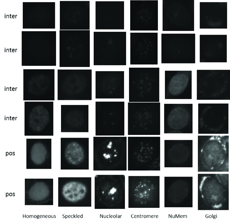
Figure 1: Sample images from all six categories in ICIP 2013 contest data set with each column from one category. The six categories are “Homogeneous”, “Speckled”, “Nucleolar”, “Centromere”, “NuMem” and “Golgi”. The first four rows show the “intermediate” samples, and the last two rows show the “positive” samples.

Recent ICPR 2012, ICIP 2013 and ICPR 2014 HEp-2 cell classification contests [13, 14, 15] have greatly put forward the development of HEp-2 cell analysis. Many features, image representation, classification methods were proposed or applied to this task. Currently, texture-based methods are the most widely used in this area. Local Binary Pattern (LBP) [16, 17, 18] is widely recognized as a discriminative texture descriptor, and widely used in face recognition [19], static and dynamic texture classification [17, 20]. Co-occurrence of adjacent LBP (CoALBP) [6], Gradient-oriented Co-occurrence of LBPs (GoC-LBPs) [7] and pairwise rotation invariant co-occurrence of LBP (PRICoLBP) [21] are three of the best performing LBP variants in HEp-2 cell classification. Besides of these three LBP variants, original LBP [17], Completed LBP (CLBP) [22] were also used in the contests. Besides of LBP based texture features, some other famous texture features, such as Maximum Response Filter Banks (e.g. MR8) [23], Gray-Level Co-occurrence Matrices (GLCM) [24], Wavelet [25], were also used in this task. We also observed that Bag of Word [26] model had been applied this task.

However, regardless of big improvement of classification accuracy in the past few years, previous works on HEp-2 cell classification task still have some limitations. Three key limitations are shown as follows:

• Previous methods pay less attention to the multi-resolution texture information. Although texture information is widely studied, the influence of multi-resolution texture analysis to HEp-2 cell classification task is unknown.

• Few works focus on capturing discriminative shape information. As far as we known, Vestergaard et al. [27] was the only work that explicitly explored the shape information in HEp-2 cell classification. Their work is different from the widely used Bag of Words (BOW) framework that our work is built on.

• The texture and shape information were considered individually, but they may be complementary to each other in practice. Thus, it will be interesting to investigate their complementary properties between them.

In this work, we attempt to address the pending issues mentioned above and hence our contributions are highlighted as follows:

• We explore the effect of multi-resolution texture for HEp-2 cell classification. To be specific, we capture the multi-resolution texture information by a novel Pairwise Rotation Invariant Co-occurrence of Local Gabor Binary Pattern (PRICoLGBP) descriptor, which is able to capture multi-resolution texture information effectively.

• We propose an effective method to depict the richer shape information by using an Improved Fisher Vector (IFV) model with RootSIFT features. Different from previous work, we extract local features from large image patches in multiple scales.

• We investigate the complementary effect of texture and shape information. By combining the multi-resolution texture and richer shape information, we yield superior classification accuracy. Compared with the winner of ICPR 2012 contest, our methods improves the accuracy of the winner by about 7%. Compared with the winner of ICIP 2013 contest, our method obtains 4% higher accuracy. Our method also achieves comparable performance to the winner of the newly release ICPR 2014 contest.

The rest of the paper is organized as follows. We firstly review the state-of-the-art methods in the HEp-2 cell classification area in Sec. II. Then, we present the proposed texture and shape features in detail in Sec. III. The used data sets are introduced in Sec. IV. In Sec. V, we firstly give a comprehensive experimental evaluations of properties of the proposed discriminative texture and shape methods, and then compare it with some state-of-the-art methods. Finally, we give a conclusion in Sec. VI.

II Related Works

II-A Best Performing Methods in ICPR 2012 Contest

Nosaka et al. [6]-the winner of ICPR 2012-only used the green channel in their method. The image was filtered by a Gaussian function to remove the noise. To improve the robustness to image rotation, they manually rotated the image to 9 orientations. Then, they extracted co-occurrence of adjacent LBP (CoALBP) features for all images (including the original images and the manually created images). Finally, they trained a linear Support Vector Machine (SVM) classifier.

The success of Nosaka’s methods is due to the following three aspects:

• Strong discriminative of CoALBP: the CoALBP was built on LBP that proves to be a powerful texture descriptor. Moreover, to capture strong spatial layout information, the CoALBP used 10 templates.

• Green channel used: Among all the three channels, green channel was much stronger than the red and blue channels. Using gray-scale image would weaken the texture information in the green channel.

• Manually creating many rotated training samples: To improve the robustness of CoALBP to image rotation, they manually rotate the imaged to 9 orientations, and created 9 new rotated training samples.

Regardless of its success on ICPR 2012 contest, this method also has some limitations. Firstly, since the CoALBP itself is not rotation invariant, thus, the CoALBP is not robust to image rotation although Nosaka et al. try to improve the CoALBP’s robustness to rotation by manually creating more rotated training samples. Secondly, the discriminative power of CoALBP is limited due to that the CoALBP is built on the co-occurrence of two LBPs with four neighbors. The LBP(4, 1) is usually considered to be less discriminative than the LBP(8, 1).

Kong et al. [8]-the second place of ICPR 2012- adopt Varma’s MR8 method to extract the texture feature. The local regions were normalized before the filter responses are applied. After feature extraction, they trained a global texton dictionary using K-means clustering. Thus, each image could be represented as a frequency histogram of textons. They also used a pyramid histogram of oriented gradients (PHOG) [28] feature to depict the shape information. The texture and shape histogram were concatenated with different weights. Finally, they used a K-Nearest Neighbor (KNN) classifier with ${\chi}^{2}$ distance.

II-B Best Performing Methods in ICIP 2013 Contest

Shen et al. [14]-the winner of ICIP 2013- combined the the original PRICoLBP and the Bag of SIFT feature. For the PRICoLBP feature, they used 10 templates. The dimension of the PRICoLBP for each template is 590. Thus, the total dimension of their used PRICoLBP feature is 5900. For the Bag of SIFT feature, following the traditional bag of words model, they created 1024 words using K-means clustering. Finally, they concatenated these two features and used linear SVM (Support Vector Machine) with square root features.

The success of this method is due to the following three aspects. Firstly, the PRICoLBP is good at capturing the texture information, meanwhile, as argued in [21], when the shape structures are strong in the data set, the utilization of 10 templates significantly improves the performance of 2 templates. Secondly, the bag of SIFT is good at capturing the global texture and shape information. Finally, the square root normalization of the feature is an effective method for linear SVM. The square root normalization has proved to be effective in many computer vision works [29].

Vestergaard et al. [27]-the merit winner of ICIP 2013- adopted a standard pipeline for the supervised image classification: preprocessing of the images, feature extraction and classification. A two-stage preprocessing method was exploited. First, each image $I$ was augmented with its logarithmic representation $loge(I)$. Then, the logarithmic representation was mapped linearly to [0,1]. For the feature extraction, Vestergaard et al. extracted three kinds of features including: 1) the “Intersity” of each image (Negative/Intermediate/Positive) as an integer flat, 2) morphological features extracted from the provided mask (containing the area of the mask region, eccentricity, major and minor axis length, perimeter); and 3) the donut-like shape index histogram feature (for both image representations). For the classification, Vestergaard et al. used a RBF kernel SVM.

II-C Best Performing Methods in ICPR 2014 Contest

Manivannan et al. [30] ranked 1st in the newly released ICPR 2014 HEp-2 cell classification contest [15]. Their method can be summarized into the following steps:

• Rotating the images to four orientations (0, 90, 180, 270) respectively;

• Dense sampling of multi-scale patches ($12\times 12,16\times 16,20\times 20$);

• Extraction of four types of features (Multi-resolution local patterns (mLP), Root-SIFT (rSIFT), Random projections (RP), Intensity histogram (IH));

• Feature encoding with Locality-constrained Linear Coding (LLC) for four types of features and four orientations individually. Thus, $4\times 4=16$ histograms can be obtained;

• Training 16 classifiers with linear SVM and Classification based on 16 classifiers.

II-D Other Relevant and Well-Performing Methods

Theodorakopoulos et al. [7] proposed a sparse representation of textural features which were fused into dissimilarity space. Along with a multivariate distribution of SIFT feature, Theodorakopoulos et al. [7] proposed a Gradient-oriented Co-occurrence of LBPs which is considered in [7] as a relaxed variation of the PRICoLBP. The descriptors were fused while creating a dissimilarity representation of an image. Finally, a sparse representation-based classification scheme was used for the classification.

In [7], the usage of SIFT feature was in a simple manner. Simple multivariate distribution of SIFT feature was used. Meanwhile, the used GoC-LBP was not robust to image rotation. Since the GoC-LBP was built on the co-occurrence of two uniform LBPs, its dimension ($59\times 59=3481$) was higher than PRICoLBP (590).

Faraki et al. [12] extended the traditional bag-of-word (BOW) from Euclidean space to non-Euclidean Riemanian manifolds that is an intrinsic bag of Riemannian words (BoRW). The BOW model has been applied to HEp-2 cell in [10] before. Faraki et al. also proposed Fisher Tensor to encode higher statistics information when building the histogram for the images. The Fisher Tensor can be seen as a Riemannian version of Fisher Vector [31]. Their proposed BoRW and its extension with Fisher Tensor in [12] demonstrate great performance on both HEp-2 cell classification and texture classification tasks.

III Hep-2 Cell Classification Using Discriminative Texture and Shape Features

This section consists of three subsections. In the first part, we introduce one novel multi-resolution texture feature. In the second part, we present our approach for depicting discriminative shape information. Finally, we describe the normalization and classification methods.

III-A Discriminative Texture Feature

III-A1 Local Binary Pattern

Local Binary Pattern (LBP) that was firstly proposed by Ojala et al. [17] is considered as a simple and effective texture descriptor. For any pixel $A$ in an image, we can compute its LBP pattern by thresholding the pixel values of its circularly symmetric $P$ neighbors with the pixel value of the central point $A$. The LBP of pixel $A$ can be defined as follows:

$$\text{LBP}_{P,R}(A)=\sum_{i=0}^{P-1}s(V_{i}-V_{c})2^{i},\ \ s(x)=\begin{cases}1,&x\geq 0\\ 0,&x<0,\\ \end{cases}$$

where $P$ is the number of the neighbors, $R$ is the radius, $V_{c}$ is the pixel value of point $A$, and $V_{i}$ is the pixel value of point $A$’s $i$th neighbor. Since the $s(V_{i}-V_{c})$ is invariant to monotonic change of illumination, thus the LBP is gray-scale invariant.

The patterns with very few spatial transitions is considered to depict the fundamental image micro-structures. Such patterns were called as “uniform patterns”. Ojala et al. [17] defined a uniformity measure for the uniform patterns, which is $\mathcal{U}(\text{LBP}_{P,R}(A))\leq N$ ($N$ is usually set to 2). The uniformity measure $\mathcal{U}(\cdot)$ can be calculated as follows:

$$\mathcal{U}(\text{LBP}_{P,R}(A))=\sum_{i=0}^{P-1}|s(V_{i}-V_{c})-s(V_{i-1}-V_{c})|,$$

where the pixel value of $V_{-1}$ is equivalent to the pixel value of $V_{P-1}$. For example, “11000000” and “10000001” are uniform patterns, and “10000100” and “10101100” are non-uniform patterns.

Rotation invariant LBP (${\text{LBP}^{ri}}$) and rotation invariant uniform LBP (${\text{LBP}^{ru}}$) are also introduced in [17]. The ${\text{LBP}^{ri}}$ can be defined as:

$$\text{LBP}_{P,R}^{ri}(A)=\text{min}\{\text{ROR}(\text{LBP}_{P,R}(A),i)\ \ |\ \ \forall i\in[0,P-1]\},$$

where $ROR(x,i)$ performs a circularly bit-wise right shift for $i$ times. The $\text{LBP}_{n,r}^{ru}(A)$ is defined as

$$\text{LBP}_{P,R}^{ru}(A)=\begin{cases}\sum_{i=0}^{P-1}s(V_{i}-V_{c}),&\mathcal{U}(\text{LBP}(A))\leq 2\\ P+1,&\text{otherwise},\\ \end{cases}$$

The $\text{LBP}_{8,1}$ has 256 patterns in total, in which 58 patterns are uniform and the rest 198 patterns are non-uniform. Usually, the 198 non-uniform patterns are summarized to one pattern. Thus, 59 patterns are usually used for uniform LBP. The rotation invariant uniform $\text{LBP}_{8,1}$ includes 10 patterns.

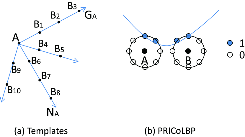
Figure 2: Pairwise Rotation Invariant Co-occurrence of Local Binary Pattern. The left of the figure shows 10 templates based on the reference point $A$. $G_{A}$ is the gradient orientation of point $A$, $N_{A}$ is the normal direction of point $A$. The right point shows one co-occurrence pair of LBPs. PRICoLBP captures stronger structures than the single LBP.

III-A2 Single-Resolution Texture Information

Pairwise rotation invariant co-occurrence LBPs (PRICoLBP) is recently introduced by Qi et al. [21] for texture related tasks. As shown in Fig. 2(a), the PRICoLBP is built on the two adjacent LBP points. Given a point $A$, the PRICoLBP contains the following two key steps to calculate its rotation invariant pattern:

• According to the gradient and normal orientation (Normal orientation is the direction that is orthogonal to the gradient orientation.) of point $A$ and pre-defined templates as shown in Fig. 2(a), the position of point $B_{i}$ can be uniquely determined. The gradient orientation can be calculated as $\theta(A)=\arctan(\frac{dy(A)}{dx(A)})$.

• With a pair $A$ and $B_{i}$, pairwise rotation invariant encoding was used to encode the co-occurrence of two LBPs.

In practice, we used the gradient magnitudes of point $A$ and $B_{i}$ to weight their co-pattern.

For the first step, given a point $A$, the PRICoLBP uses the following equation to determine the position of point $B_{i}$:

$$B_{i}=a_{i}*G(A)+b_{i}*N(A)+A,$$ (1)

where $a_{i}$ and $b_{i}$ are pre-defined coefficients for template $i$, and $G(A)$ and $N(A)$ are the gradient and normal directions of point $A$. In practice, we can choose 10 pairs for [$a_{i}$, $b_{i}$] as shown in Fig. 2(a), one pair corresponds to one template.

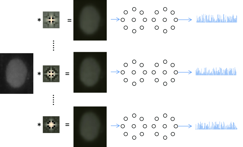
Figure 3: The framework of PRICoLGBP. First, the image is filtered by Gabor filters with different scales. Then, the PRICoLBP features are extracted from each filtered images. Finally, the features extracted from each scale will be concatenated into the final feature.

When the point pair $A$ and $B_{i}$ are determined, a pairwise rotation invariant encoding strategy is used to encode the pair. Denote $\text{LBP}^{u}(A,i)$ as the uniform LBP of point $A$ by using $i$-th index as the start point of the binary sequence. The PRICoLBP can be defined as follows:

$$\text{PRICoLBP}_{P,R}(A,B_{i})=[\text{LBP}_{P,R}^{ru}(A),\text{LBP}_{P,R}^{u}(B_{i},i(A))]_{co},$$ (2)

where $i(A)\in\{0,P-1\}$ is an index, which can be determined by minimizing the binary sequence of point $A$. $[\ ,\ ]_{co}$ is a co-occurrence operator firstly introduced in [24]. Suppose $\text{LBP}_{P,R}^{ru}(A)$ has $M$ patterns, and $\text{LBP}_{P,R}^{u}(B_{i},i(A))$ has $N$ patterns, then their co-occurrence has $M\times N$ patterns.

For one pair $A$ and $B_{i}$ with $P=8$ and $R=1$, $\text{LBP}_{8,1}^{ru}(A)$ has 10 patterns, $\text{LBP}_{8,1}^{u}$ has 59 patterns, thus, the dimension of $\text{PRICoLBP}_{8,1}$ is $10\times 59=590$. If 10 templates are used as shown in Fig. 2(a), the dimension for PRICoLBP is $10\times 590=5900$.

III-A3 Multi-Resolution Texture Information

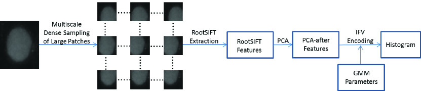
Figure 4: The framework of discriminative shape information description. First, we densely sample thousands of large patches in multiple scales with a preset step (such as 2), then the RootSIFT feature is extracted for each patch. PCA is applied to the RootSIFT. Finally, IFV encoding is applied to the PCA-after features with pre-learned GMM parameters. The obtained histogram from IFV encoding can be input into a linear SVM for the final classification.

The PRICoLBP is effective to capture the structures in the small scales (such as co-occurrence of $\text{LBP}_{8,1}$ and co-occurrence of $\text{LBP}_{(}8,2)$), but texture information in large scales is ignored. However, multi-resolution texture information is always effective for many vision applications.

To capture multi-resolution texture information, we propose a novel pairwise rotation invariant co-occurrence of local Gabor binary pattern (PRICoLGBP) descriptor. Gabor wavelet [25] [32] is an effective filter to capture multi-resolution and multi-orientation information. The PRICoLGBP is built on the Gabor filter and PRICoLBP descriptor. The framework of our PRICoLGBP can be seen in Fig. 3. We convolute the original image with different Gabor filters, and then extract the PRICoLBP from each filtered image, and finally concatenate all PRICoLBPs into the final feature. In experiments, we found that the PRICoLGBP is not sensitive to rotation variation for the Gabor filtered images, thus, we only use one pre-fixed orientation for all scales.

The PRICoLGBP shares some similar properties with Local Gabor Binary Pattern (LGBP) [33] that is seen as a powerful LBP variants in face recognition, but different from the LGBP, our PRICoLGBP is built on a more discriminative co-occurrence of LBPs features. Thus, we can expect that PRICoLGBP can capture stronger multi-resolution texture information.

We believe two strong properties of the PRICoLGBP makes it effective for IIF HEp-2 cell classification.

• PRICoLGBP has strong texture discrimination. In IIF HEp-2 cell classification, texture-based methods proves to be effective.

• Gabor and PRICoLBP both are robust to image illumination variation. PRICoLGBP inherited the properties from both Gabor and PRICoLBP. In IIF HEp-2 cells, the “Positive” and “Intermediate” cells from the same categories show extremely varying illumination.

III-B Effective Shape Feature

In this subsection, we present an effective method to depict the richer shape information by using an Improved Fisher Vector (IFV) model with RootSIFT features extracted from large image patches in multiple scales. Our approach consists of three steps: a) patch sampling, b) feature description with RootSIFT, and c) encoding by IFV. The flowchart to illustrate our approach is displayed in Fig. 4.

III-B1 Patch Sampling for Depicting Shape Information

To increase the discriminativeness in shape information, we propose to sample large patches, since that the large patches preserve stronger shape structures. To be specific, instead of sampling patches of small size, e.g., $16\times 16$, $17\times 17$, or $19\times 19$ as in object categorization tasks, we sample much larger patches, e.g., $41\times 41$. We can observe in Fig. 4 that the sampled patches cover more than $\frac{1}{3}$ of the whole image.

Figure 5: Illustration of discrimination of shape information in ICIP 2013 contest data set. Each column comes from one category. It is easy to find that the shapes vary a lot among different categories. (A) shows the “Intermediate” cell images from each category, and (B) shows (A)’s corresponding enhanced images from a logarithmic operator $loge(I)$. (C) shows the “Positive” cell images, and (D) is (C)’s corresponding enhanced images.

In Fig. 5, we show some samples from all six categories in ICIP 2013 contest data set.

• The shape structures from different categories change a lot. Each category has its own basic characteristics. For instance, the category “NuMum” has bright and thick boundary, the category “Centermere” has many bright spots, and the category “Golgi” does not have well-formed boundary. Considering local texture structures, the shape difference between some categories is large. For instance, the categories “Nucleolar” and “Centromere” are easy to differentiate when jointly considering the shape and texture.

• The “positive” and “intermediate” HEp-2 cells from same category share similar shape structure, although we cannot see the shape structure of the “intermediate” HEp-2 cells clearly.

These observations are the rationales to explore the shape information for HEp-2 cell image classification.

III-B2 RootSIFT Feature Extraction on Large Patches

We extract 128-dimensional SIFT features [34] from the sampled large patches. For each SIFT feature $\bf f$, we normalize it with $L_{1}$-norm and then take the componentwise square root operation, i.e.,

$$\begin{split}\bar{\bf f}&={\bf f\over\|\bf f\|_{1}},\\ \tilde{f}_{j}&=\sqrt{\bar{f}_{j}},~{}~{}~{}~{}j=1,\cdots,128.\end{split}$$ (3)

The obtained $\tilde{f}$ is termed as “RootSIFT” [35], which was proposed by Relja et al. to enhance the discriminative power of SIFT.

III-B3 Improved Fisher Vector (IFV) for Encoding the RootSIFTs

We encode the RootSIFT features by Improved Fisher Vector (IFV) approach [31] [36], which consists of three steps:

• Data decorrelation by Principal Component Analysis (PCA).

• Training a Gaussian Model of Mixture (GMM).

• Forming the IFV by using the first and second order statistics in GMM.

Denote the parameters in GMM as $\{\pi_{k},\mu_{k},\Sigma_{k}\}_{k=1}^{K}$ where $\pi_{k}$ is the membership probability, $\mu_{k}$ is the mean of $k$-th component Gaussian, and $\Sigma_{k}$ is the covariance matrix which is enforced to be diagonal. Let $X=[\textbf{x}_{1},\textbf{x}_{2},...,\textbf{x}_{N}]\in\mathcal{R}^{d\times{N}}$ be a set of feature vectors of an image after decorrelation, where $d$ is reduced feature dimension of using PCA and $N$ is the number of RootSIFT features in the image. IFV captures the deviation of the features in an image from the first and second statistics of the GMM. To be specific, IFV is defined as follows:

$${\bf{F}}=[{{\bf{u}}_{1}}^{\rm{T}},{\bf{v}}_{1}^{\rm{T}},...,{\bf{u}_{K}}^{\rm{T}},{\bf{v}_{K}}^{\rm{T}}]^{\rm{T}},$$ (4)

where

$${\bf{u}}_{k}=\frac{1}{N\sqrt{{\pi}_{k}}}\sum_{i=1}^{N}s_{ki}{{\Sigma}_{k}}^{-\frac{1}{2}}(x_{i}-\mu_{k}),$$ (5)

$${\bf{v}}_{k}=\frac{1}{N\sqrt{2{\pi}_{k}}}\sum_{i=1}^{N}s_{ki}[(x_{i}-\mu_{k})\cdot({{\Sigma}_{k}}^{-1}(x_{i}-\mu_{k}))-{\bf{1}}],$$ (6)

in which $s_{ki}$ is defined as

$$s_{ki}=\frac{p(x_{i}|\mu_{k},{\Sigma}_{k}){\pi}_{k}}{\sum_{i=1}^{K}p(x_{i}|\mu_{i},{\Sigma}_{k})){\pi}_{i}},\ \ \ \ \ \ k=1,...,K.$$

The parameter $s_{ki}$ is the responsibility of feature $\textbf{x}_{i}$ belonging to the $k$-th component in the GMM.

Note that the dimension of ${\bf{F}}$ is $2\times{d}\times{K}$.In our experiments, we set $d$ as 80, and $K$ as 256, the number of mixture components in GMM. The final dimension of IFV feature is $2\times 80\times 256=41960$. Note also that this is the first time that IFV is used in HEp-2 cell classification task.

III-C Histogram Normalization and Classification

Histogram normalization is a key step before training a SVM model. We normalize the histogram componentwisely as follows:

$$\hat{H}_{i}=sign(H_{i})\sqrt{\mid{H_{i}}\mid},\forall i=1,\cdots,D,$$ (7)

where $D$ is the dimension of $H$, $sign(\cdot)$ is a sign function. And then we further normalize the histogram with $L_{2}$ norm.

For classification we use linear SVM since it is widely used in large scale problems. For linear SVM, the training is fast and the speed of classification in test phase is also fast, compared to kernel SVM. We use the one-vs-the-rest strategy to handle the multi-class classification problem.

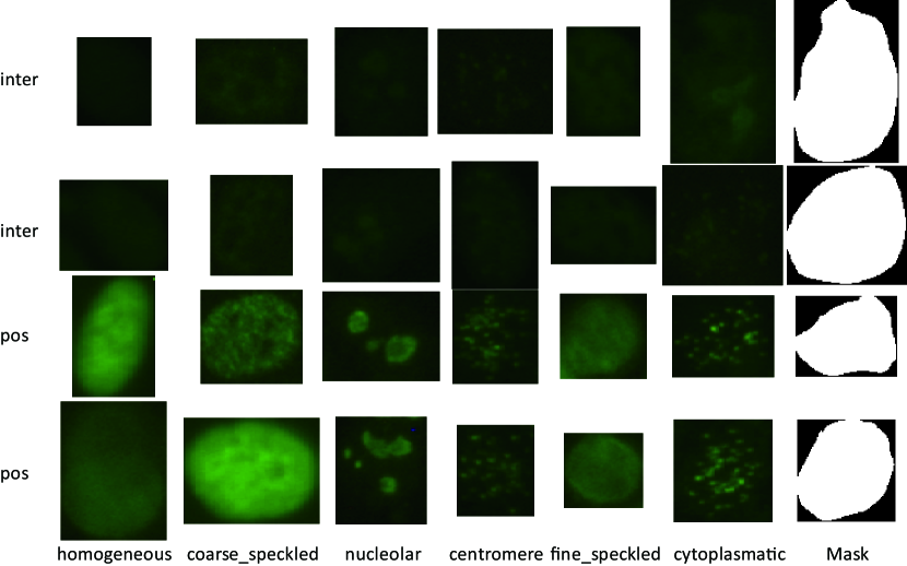
Figure 6: Sample images from ICPR 2012 contest dataset with each column from one category. The first two rows show the intermediate samples, and the last two rows show the positive samples. All the images are shown in their original image size.

IV Datasets and Evaluation Metrics

TABLE I: Details of ICPR 2012 contest data set.

	Homo	Coar	Fine	Nucl	Cent	Cyto	Total
Instances/train	3	2	2	2	3	2	14
Cells/train	150	109	94	102	208	60	723
Instances/test	2	3	2	2	3	2	14
Cells/test	180	101	114	139	149	51	734

IV-A ICPR 2012 Contest Dataset

ICPR 2012 cell images were acquired by means of a fluorescence microscope (40-fold magnification) coupled with a 50W mercury vapor lamp and with a digital camera. The images have a resolution of $1388\times 1038$ pixels, a color depth of 24 bits and they are stored in an uncompressed format. Specialists manually segmented and annotated each cell. In particular, a biomedical engineer manually segmented the cells by the use of a tablet PC. Subsequently, each image was verified and annotated by a medical doctor specialized in immunology. The dataset contains 28 images almost equally distributed with respect to the different patterns. In the contest, the 28 images are divided into training and testing sets. The information for training and testing sets is shown in Tab. I. More detailed information can be found in [13]. Some samples are shown in Fig. 6.

Note that a specimen always has dozens of cells. The cells in the same specimen always have higher similarity than that of the cells from different specimens. Thus, to evaluate the generalization ability of the methods, the cells in one specimen can only be used for training or testing, it will be misleading to split them into training and testing. In the ICPR 2012 contest report, several methods used this strategy and directly splits all cell images instead of the specimens into training and validation sets, but their final results reported by the organizers were significantly lower than the authors’ reported results.

IV-B ICIP 2013 Contest Dataset

The ICIP 2013 data set uses 419 patients positive sera with screening dilution 1:80. The specimens were automatically captured using a monochrome high dynamic range cooled microscopy camera. For each patient serum, 100-200 cell images were extracted. In total, there were 68429 cell images extracted. The whole 68429 cell images were divided into 13596 training samples and 54833 testing samples.

TABLE II: Details of ICIP 2013 contest data set.

	Ho	Sp	Nu	Ce	NM	Go	Total
Specimens	16	16	16	16	15	4	83
Cells	2494	2831	2598	2741	2208	724	13596

The labeling process involved at least two scientists who read each patient’s specimen under a microscope. A third expert’s opinion was sought to adjudicate any discrepancy between the two opinions. In this way, a ground-truth mask can be extracted from each cell image.

The testing images are not released. But the training set is big enough to evaluate different algorithms. Some basic information for the training data in ICIP 2013 contest are shown in Tab. II. More detailed information can be found in [14]. Some sample images are shown in Fig. 1.

It should be noted that in ICPR 2014 contest, the Task-1 used the same dataset as ICIP 2013 contest.

IV-C Evaluation Metrics

In the previous ICPR 2012 and ICIP 2013 contests, accuracy of maximum classification number is used as a performance metric. For specimen, in ICPR 2012 data set, the testing number of images are 734, if the 500 images are classified correctly, then the accuracy is $\frac{500}{734}$. In this paper, we follow the metric of the previous ICPR 2012 and ICIP 2013 contest, and use the maximum classification number as the metric.

When comparing our method with ICPR 2014 winner [30], we strictly follow the winner’s protocol, and use the leave-one-specimen-out protocol. The averaged Mean Class Accuracy (MCA) is reported.

V Experiments

V-A Implementation Details

PRICoLGBP. For multi-resolution PRICoLGBP feature, we use the original image and 7 Gabor-filtered images under 7 different scales $\{1,2,3,4,5,6,7\}$. For each filtered image, we can extract one PRICoLBP feature. In each PRICoLBP feature, we use 10 templates. As we described before, the dimension of PRICoLBP using one template is 590. Thus, the final dimension for PRICoLGBP is $8\times 10\times 590=47200$.

RootSIFT(IFV). We densely sample the RootSIFT feature at six scales with grid step 2. The sampled patch size is $41\times 41$. If the image size (height or width) is less 64, we will resize it to the image with minimum size 64 and keep the height/width ratio. Six scales are achieved by filtering the images with Gaussians with different scales of different standard deviates $\{{1.5},{1.5}^{2},{1.5}^{3},{1.5}^{4},{1.5}^{5},{1.5}^{6}\}$. For specimen, for an image with image size $70\times 70$, we can sample 225 points for each scale. Thus, for six scales, we can get 1350 sampled patches. For a larger image, such as $70\times 80$, we will sample more points. In the IFV, we firstly sample 100000 RootSIFT features from the training samples, then the 100000 RootSIFT features are used to learn the PCA components, and 80 principal components are preserved as the basis for dimension reduction. As pointed out by [36], the PCA is a key step in the IFV framework. With above-mentioned 100000 after-PCA RootSIFT feature, we learn a Gaussian Mixture Model (GMM) with 256 components. For the PCA, we use the built-in SVD (Singular Value Decomposition). For the GMM, we use Vlfeat to learn the parameters $\theta=\left\{\pi_{k},\mu_{k},\Sigma_{k},k=1,\cdots,K\right\}$. The final dimension using the IFV encoding is $2\times 80\times 256=41960$.

Experimental Setups. Vlfeat toolbox [37] is used for fast RootSIFT extraction and IFV encoding, and Liblinear [38] is used for the linear SVM training and classification. For the parameter C, we cross-validated it in {0.001, 0.01, 0.1, 1, 100, 1000}. It should be noted that the first author of this paper provides PRICoLBP feature and classifier for Shen et al. (the ICIP 2013 winner). We share the source code that had been submitted into ICIP 2013 and achieved the 1st place. All experimental comparisons are conducted in the same framework. Take ICIP 2013 contest data set as example, first, we create 10 splits for 10 repeated experiments. For each split, the whole ICIP contest 2013 data set are randomly divided into the training and testing sets. Meanwhile, to truly show the generalization performance of approaches, the images from the same cell are only divided into training or testing set. Thus, All comparisons are fair in this paper. We have provided the matlab code to repeat the experimental results.

V-B Evaluation of Features

In this subsection, we will mainly evaluate some aspects of the proposed texture and shape features. The ICPR 2012 data set is too small to fully evaluate the properties of the proposed methods. Thus, we will use ICIP 2013 data set in this subsection. To fully evaluate the properties, we use four sets of different experimental setups, as shown in Tab. III. Take the setup “D” as an example, in experimental setup “D”, 42 specimens (including 8 specimens from “Homogeneous”, 8 specimens from “Speckled”, 8 specimens from “Nucleolar”, 8 specimens from “Centromere”, 8 specimens from “NuMem” and 2 specimens from “Golgi”) in all 83 specimens are used for training, and the rest 41 specimens are used for testing, each specimen includes 100-200 cell images. Using this strategy, the images in one specimen can only be divided into training or testing. This used strategy can truly reflect the generalization ability because the images come from the specimen usually have higher similarity than that between images from different specimen, if part of the images in one specimen are used for training, the rest images that are used for testing are easily correctly classified, but this strategy can not be generalized to other unknown specimen. We pre-create 10 training and testing splits randomly. We repeat the experiments 10 times and average the results.

TABLE III: Four experimental setups for ICIP 2013 data set. For example, “1” means all images from one specimen are used for training, and the remaining specimens are used for testing.

	Ho	Sp	Nu	Ce	NM	Go	total
Setup A	1	1	1	1	1	1	6
Setup B	2	2	2	2	2	2	12
Setup C	4	4	4	4	4	2	22
Setup D	8	8	8	8	8	2	42

Evaluation of Multi-Resolution Texture Extraction Strategy. Here, we conduct experiments to compare the PRICoLBP and PRICoLGBP on above-mentioned four experimental setups. The results are shown in Tab. IV.

TABLE IV: Comparison between the single-resolution and multi-resolution texture feature on ICIP 2013 data set.

	Setup A	Setup B	Setup C	Setup D
PRICoLBP	$43.1\pm{6.8}$	$55.2\pm{5.4}$	$67.6\pm{4.0}$	$73.9\pm{2.9}$
PRICoLGBP	$50.4\pm{6.2}$	$61.4\pm{5.1}$	$72.2\pm{3.8}$	$78.4\pm{2.7}$

We can observe that from Tab. IV, multi-resolution texture feature significantly improves the single-resolution texture feature. For specimen, the multi-resolution PRICoLGBP improves the PRICoLBP by 7.3% and 4.5% for the experimental setup “A” and “D”.

Evaluation of Improved Fisher Vector Encoding. To evaluate the effectiveness of the Improved Fisher Vector, we compare it with the traditional Vector Quantization (VQ). For both VQ and IFV, the feature is normalized according to Eq. 7. A linear SVM is used for training and classification. The results averaged on 10 random repeats are shown in Tab. V.

TABLE V: Comparison between Vector Quantization and Improved Fisher Vector on ICIP 2013 data set.

	Setup A	Setup B	Setup C	Setup D
RootSIFT(VQ)	$54.9\pm{6.8}$	$62.2\pm{4.5}$	$68.3\pm{2.4}$	$71.2\pm{2.3}$
RootSIFT(IFV)	$58.7\pm{6.7}$	$66.7\pm{5.1}$	$74.7\pm{2.7}$	$78.4\pm{2.7}$

From Tab. V, we can find that the IFV encoding method sharply improves the performance of the VQ encoding method. For specimen, under the experimental configuration “D”, the IFV improves the VQ from 71.2% to 78.4%. In conclusion, the IFV is an effective way to preserve the discriminative power of the features under the BoW framework.

Evaluation of Normalization Method. Here, we evaluate the importance of the normalization method. For both PRICoLGBP feature and RootSIFT(IFV), we normalized the histograms according to Eq. 7. We compare them with the direct $L_{2}$ normalized histograms(without using Eq. 7) under the linear SVM framework. The results averaged on 10 random repeats are shown in Tab. VI.

TABLE VI: Evaluation of Normalization Methods on RootSIFT(IFV) and PRICoLGBP on ICIP 2013 data set. In the table, “PRICoLGBP” and “RootSIFT(IFV)” denotes the feature under the direct $L_{2}$ normalization, “PRICoLGBP*” and “RootSIFT(IFV*)” denotes the features normalized by Eq. 7 and then by $L_{2}$ normalization.

	Setup A	Setup B	Setup C	Setup D
PRICoLGBP	$48.4\pm{6.2}$	$59.4\pm{4.6}$	$70.3\pm{3.2}$	$77.5\pm{3.2}$
PRICoLGBP*	$50.4\pm{6.2}$	$61.4\pm{5.1}$	$72.2\pm{3.8}$	$78.4\pm{2.7}$
RootSIFT(IFV)	$57.8\pm{7.0}$	$65.7\pm{5.4}$	$73.6\pm{2.9}$	$77.4\pm{2.7}$
RootSIFT(IFV*)	$58.7\pm{6.7}$	$66.7\pm{5.1}$	$74.7\pm{2.7}$	$78.4\pm{2.7}$

From Tab. VI, it is easy to find that the PRICoLGBP with normalization according to Eq. 7 consistently outperforms the PRICoLGBP without normalization, and the RootSIFT(IFV) using normalization also consistently outperforms the non-normalized feature. In conclusion, the normalization always improves the classification accuracy.

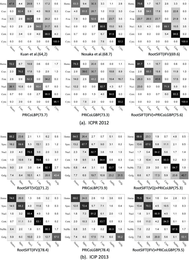
Figure 7: Classification confusion matrixs and averaged accuracies on (a). ICPR 2012 and (b) ICIP 2013 contest data sets.

V-C Comparison with the State-of-the-art Methods

Experiments on ICPR 2012 contest. For this dataset, we evaluate seven methods, including PRICoLBP, PRICoLGBP, RootSIFT(IFV), the combination of PRICoLGBP and RootSIFT(IFV), and the top three methods in ICPR 2012 contest. For PRICoLBP and PRICoLGBP, we use the green channel. For RootSIFT(IFV), we use the gray image. In IFV, since the sampled patch is $41\times 41$, when the minimal size of the image is less than 50, we will resize the image to the minimal size 64 while keeping the ratio between the height and width. Since the dataset is very small, for the PRICoLBP and PRICoLGBP, we directly use SVM with ${\chi}^{2}$ kernel. For the RootSIFT(IFV), and the combination of PRICoLGBP and RootSIFT(IFV), we use linear SVM. The classification confusion matrix and averaged accuracies using the provided experimental setup by the ICPR 2012 contest organizers are shown in Fig. 7(a).

We have the following observations from Fig. 7(a):

• Texture based methods works better than the shape based methods. For specimen, PRICoLBP achieves 73.7% which is higher than RootSIFT(IFV) (69.6%).

• IFV encoding with RootSIFT works well on this dataset, and slightly outperforms winner of ICPR 2012 contest.

• The combination of our PRICoLGBP and RootSIFT(IFV) significantly outperforms the winner of ICPR 2012, and performs better than the latter on four categories including “Homogeneous”, “Coarse Speckled”, “Centromere” and “Cytoplasmic”, and worse on the categories “Nucleolar” and “Fine Speckled”.

It should be noted that the experimental results on ICPR contest dataset are sensitive to the classifier’s parameter C. We used the training set to conduct cross-validation to get a good C. Since the number of all specimens in ICPR 2012 contest is limited, thus, we use leave-one-out strategy to make cross-validation.

Experiments on ICIP 2013 contest. We evaluate and compare six methods including RootSIFT(VQ), PRICoLBP, the combination of RootSIFT with VQ and PRICoLBP, PRICoLGBP, RootSIFT(IFV), and the combination of PRICoLGBP and RootSIFT(IFV). Here, we use the experimental setup “D”. The features are all normalized, and a linear SVM. The classification confusion matrix and averaged accuracies based on 10 random repeats are shown in Fig. 7(b).

The confusion matrix in Fig. 7(b) indicates that:

• Multi-resolution PRICoLGBP texture feature significantly outperforms the single-resolution PRICoLBP, and improves the performance from 73.9% to 78.4%. PRICoLGBP significantly improves the PRICoLBP on several categories such as “Speckled” and “Golgi”, and has high performance on other categories. Compared with RootSIFT(VQ), RootSIFT(IFV) significantly outperforms the former on all categories. This fully demonstrates the effectiveness of IFV encoding methods.

• The combination between texture and shape features outperforms each of them. For specimen, the combination of RootSIFT(VQ) and PRICoLBP improves the PRICoLBP (73.9%) and RootSIFT(VQ) (71.2%) to 75.3%. And, the combination of PRICoLGBP and RootSIFT(IFV) greatly improves the Shen’s method (the winner of ICIP 2013) from 75.3% to 79.5%.

• The category “Golgi” obtains the lowest performance, this is due to the less training sampling in this category. The most confusing pairs are “Golgi” and “Nucleolar”, and “Speckled” and “Homogeneous”. It is easy to find that from Fig. 1, the shape and texture structures in “Homogeneous” and “Speckled” look similar.

Comparision with the Winner of ICPR 2014 contest. Recently, the results of ICPR 2014 HEp-2 Cell classification have been released. In this part, we compare our method with the winner of ICPR 2014 contest [30]. We strictly follow the experimental protocol of the winner, and use the leave-one-specimen-out strategy. According to the specimen IDs, we can split the data into training and validation sets. Since we have 83 different specimens, in each test, we use 82 specimens for training and the left one for testing. The result of the ICPR 2014 winner is shown in Table VII(a), and our result based on PRIGCoLBP and RootSIFT(IFV) is shown in Table VII(b).

According to Table VII, the Mean Class Accuracy (MCA) for the winner of ICPR 2014 contest is 80.25%, and our method achieves a comparable performance 80.04%. It should be noted that Manivannan et al. used four types of features, and for each feature, they trained 4 models, and the final classification result is based on summation of probability of 16 classifier. However, we only trained one model using the combination of the RootSIFT (IFV) and PRICoLGBP features. We can find that our method performs better on “Nucleolar” and “Golgi”, and performs worse on “Homogeneous”, “Speckled” and “Centromere”.

TABLE VII: Confusion matrixs of (a). the ICPR 2014 Contest Winner, and (b). Our method for leave-one-specimen-out experiments on I3A Task-1 dataset.

(a). The winner of ICPR 2014 contest.
	Homo.	Spec.	Nucl.	Cent.	NuMe.	Golgi
Homo.	81.8	15.00	0.76	0.20	2.04	0.20
Spec.	8.87	77.36	3.67	9.18	0.74	0.18
Nucl.	1.12	3.89	90.65	2.08	1.27	1.00
Cent.	0.47	10.87	2.85	85.66	0.04	0.11
NuMe.	6.30	2.04	1.40	0.27	88.04	1.95
Colgi.	5.66	3.73	20.72	2.35	9.53	58.01
(b). Our method.
	Homo.	Spec.	Nucl.	Cent.	NuMe.	Golgi
Homo.	81.32	15.56	0.80	0.12	1.96	0.24
Spec.	12.19	73.86	3.74	9.29	0.78	0.14
Nucl.	1.58	2.23	92.49	2.19	0.92	0.58
Cent.	0.15	10.98	3.43	85.41	0	0.04
NuMe.	6.52	1.54	1.27	0.05	88.04	2.58
Colgi.	8.56	4.70	19.34	3.31	4.97	59.12

VI Conclusion

We have proposed an efficient and effective method for automatic classification of HEp-2 cell via using multiresolution texture and richer shape information. Specifically, we proposed to capture the multi-resolution texture information by a novel Pairwise Rotation Invariant Co-occurrence of Local Gabor Binary Pattern (PRICoLGBP) descriptor, depict the richer shape information by using an Improved Fisher Vector (IFV) model with RootSIFT features which are sampled from large image patches in multiple scales, and combine them properly. We have systematically evaluated the proposed approach on the ICPR 2012, ICIP 2013, and ICPR 2014 contest data sets. The proposed approach significantly outperformed the winners of ICPR 2012 and ICIP 2013 contests, and yileded comparable performance with the winner of the newly released ICPR 2014 contest.

VII Acknowledgment

The authors would like to thank Andrea Vedaldi for sharing the Vlfeat toolbox, and Rong-En Fan et al. for sharing the Liblinear toolbox. We also want to thank the organizer of ICPR 2012 and ICIP 2013 HEp-2 Cell classification contests for releasing the HEp-2 cell data sets. These two contests substantially put forward the research on HEp-2 cell classification. This work was supported by the Academy of Finland and Infotech Oulu.

References

- [1] P. Foggia, G. Percannella, P. Soda, and M. Vento, “Benchmarking hep-2 cells classification methods.” IEEE Transactions on Medical Imaging, vol. 32, no. 10, p. 1878, 2013.
- [2] P. Foggia, G. Percannella, A. Saggese, and M. Vento, “Pattern recognition in stained hep-2 cells: Where are we now?” Pattern Recognition, vol. 47, no. 7, pp. 2305–2314, 2014.
- [3] P. Foggia, G. Percannella, P. Soda, and M. Vento, “Early experiences in mitotic cells recognition on hep-2 slides,” in IEEE 23rd International Symposium on Computer-Based Medical Systems (CBMS), 2010, pp. 38–43.
- [4] G. Percannella, P. Soda, and M. Vento, “A classification-based approach to segment hep-2 cells,” in IEEE 25th International Symposium on Computer-Based Medical Systems (CBMS). IEEE, 2012, pp. 1–5.
- [5] I. Theodorakopoulos, D. Kastaniotis, G. Economou, and S. Fotopoulos, “Hep-2 cells classification via fusion of morphological and textural features,” in IEEE 12th International Conference on Bioinformatics & Bioengineering (BIBE). IEEE, 2012, pp. 689–694.
- [6] R. Nosaka and K. Fukui, “Hep-2 cell classification using rotation invariant co-occurrence among local binary patterns,” Pattern Recognition, vol. 47, no. 7, pp. 2428–2436, 2014.
- [7] I. Theodorakopoulos, D. Kastaniotis, G. Economou, and S. Fotopoulos, “Hep-2 cells classification via sparse representation of textural features fused into dissimilarity space,” Pattern Recognition, vol. 47, no. 7, pp. 2367–2378, 2014.
- [8] X. Kong, K. Li, J. Cao, Q. Yang, and L. Wenyin, “Hep-2 cell pattern classification with discriminative dictionary learning,” Pattern Recognition, vol. 47, no. 7, pp. 2379–2388, 2014.
- [9] L. Shen, J. Lin, S. Wu, and S. Yu, “Hep-2 image classification using intensity order pooling based features and bag of words,” Pattern Recognition, vol. 47, no. 7, pp. 2419–2427, 2014.
- [10] A. Wiliem, Y. Wong, C. Sanderson, P. Hobson, S. Chen, and B. C. Lovell, “Classification of human epithelial type 2 cell indirect immunofluoresence images via codebook based descriptors,” in 2013 IEEE Workshop on Applications of Computer Vision (WACV). IEEE, 2013, pp. 95–102.
- [11] X.-H. Han, J. Wang, G. Xu, and Y.-W. Chen, “High-order statistics of micro-texton for hep-2 staining pattern classification,” IEEE Transactions on Biomedical Engineering, 2014.
- [12] M. Faraki, M. T. Harandi, A. Wiliem, and B. C. Lovell, “Fisher tensors for classifying human epithelial cells,” Pattern Recognition, vol. 47, no. 7, pp. 2348–2359, 2014.
- [13] P. Foggia, G. Percannella, P. Soda, and M. Vento, “Hep-2 cells classification contest website [online],” in Available: http:// mivia.unisa.it/hep2contest/.
- [14] P. Hobson, G. Percannella, M. Vento, and A. Wiliem, “http://nerone.diiie.unisa.it/contest-icip-2013-test/index.shtml.”
- [15] B. Lovell, G. Percannella, M. Vento, and A. Wiliem, “Icpr 2014 hep-2 cells classification workshop and contest,” in Available: http://i3a2014.unisa.it/.
- [16] T. Ojala, M. Pietikäinen, and D. Harwood, “A comparative study of texture measures with classification based on featured distributions,” Pattern Recognition, vol. 29, no. 1, pp. 51–59, 1996.
- [17] T. Ojala, M. Pietikainen, and T. Maenpaa, “Multiresolution gray-scale and rotation invariant texture classification with local binary patterns,” IEEE Transactions on Pattern Analysis and Machine Intelligence, vol. 24, no. 7, pp. 971–987, 2002.
- [18] M. Pietikäinen, A. Hadid, G. Zhao, and T. Ahonen, Computer vision using local binary patterns. Springer, 2011, vol. 40.
- [19] T. Ahonen, A. Hadid, and M. Pietikainen, “Face description with local binary patterns: Application to face recognition,” IEEE Transactions on Pattern Analysis and Machine Intelligence, vol. 28, no. 12, pp. 2037–2041, 2006.
- [20] G. Zhao and M. Pietikainen, “Dynamic texture recognition using local binary patterns with an application to facial expressions,” IEEE Transactions on Pattern Analysis and Machine Intelligence, vol. 29, no. 6, pp. 915–928, 2007.
- [21] X. Qi, R. Xiao, C.-G. Li, Y. Qiao, J. Guo, and X. Tang, “Pairwise rotation invariant co-occurrence local binary pattern,” IEEE Transactions on Pattern Analysis and Machine Intelligence, 2014.
- [22] Z. Guo, L. Zhang, and D. Zhang, “A completed modeling of local binary pattern operator for texture classification,” IEEE Transactions on Image Processing, vol. 19, no. 6, pp. 1657–1663, 2010.
- [23] M. Varma and A. Zisserman, “A statistical approach to texture classification from single images,” International Journal of Computer Vision, vol. 62, no. 1-2, pp. 61–81, 2005.
- [24] R. M. Haralick, K. Shanmugam, and I. H. Dinstein, “Textural features for image classification,” IEEE Transactions on Systems, Man and Cybernetics, no. 6, pp. 610–621, 1973.
- [25] D. Gabor, “Theory of communication. part 1: The analysis of information,” Journal of the Institution of Electrical Engineers-Part III: Radio and Communication Engineering, vol. 93, no. 26, pp. 429–441, 1946.
- [26] G. Csurka, C. Dance, L. Fan, J. Willamowski, and C. Bray, “Visual categorization with bags of keypoints,” in European Conference on Computer Vision Workshop on Statistical Learning in Computer Vision, vol. 1, 2004, p. 22.
- [27] B. L. L. Anders, S. V. Jacob, and L. Rasmus, “Hep-2 cell classification using shape index histograms with donut-shaped spatial pooling,” IEEE Transactions on Medical Imaging, 2014.
- [28] A. Bosch, A. Zisserman, and X. Munoz, “Representing shape with a spatial pyramid kernel,” in ACM International Conference on Image and Video Retrieval. ACM, 2007, pp. 401–408.
- [29] A. Vedaldi and A. Zisserman, “Efficient additive kernels via explicit feature maps,” IEEE Transactions on Pattern Analysis and Machine Intellingence, vol. 34, no. 3, 2011.
- [30] S. Manivannan, W. Li, S. Akbar, R. Wang, J. Zhang, and S. J. McKenna, “Hep-2 cell classification using multi-resolution local patterns and ensemble svms,” in IEEE International Conference of Pattern Recognition Workshop on Pattern Recognition Techniques for Indirect Immunofluorescence Images (I3A).
- [31] F. Perronnin, J. Sánchez, and T. Mensink, “Improving the fisher kernel for large-scale image classification,” in European Conference on Computer Vision 2010. Springer, 2010, pp. 143–156.
- [32] J. R. Movellan, “Tutorial on gabor filters.”
- [33] W. Zhang, S. Shan, W. Gao, X. Chen, and H. Zhang, “Local gabor binary pattern histogram sequence (lgbphs): A novel non-statistical model for face representation and recognition,” in IEEE International Conference on Computer Vision (ICCV), vol. 1. IEEE, 2005, pp. 786–791.
- [34] D. G. Lowe, “Distinctive image features from scale-invariant keypoints,” International Journal of Computer Vision, vol. 60, no. 2, pp. 91–110, 2004.
- [35] R. Arandjelovic and A. Zisserman, “Three things everyone should know to improve object retrieval,” in IEEE Conference on Computer Vision and Pattern Recognition (CVPR). IEEE, 2012, pp. 2911–2918.
- [36] J. Sánchez, F. Perronnin, T. Mensink, and J. Verbeek, “Image classification with the fisher vector: Theory and practice,” International Journal of Computer Vision, pp. 1–24, 2013.
- [37] A. Vedaldi and B. Fulkerson, “Vlfeat: An open and portable library of computer vision algorithms,” in ACM Multimedia, 2010, pp. 1469–1472.
- [38] R. Fan, K. Chang, C. Hsieh, X. Wang, and C. Lin, “Liblinear: A library for large linear classification,” Journal of Machine Learning Research, 2008.