A Full Multigrid Method for Nonlinear Eigenvalue Problems

Abstract

This paper is to introduce a type of full multigrid method for the nonlinear eigenvalue problem. The main idea is to transform the solution of nonlinear eigenvalue problem into a series of solutions of the corresponding linear boundary value problems on the sequence of finite element spaces and nonlinear eigenvalue problems on the coarsest finite element space. The linearized boundary value problems are solved by some multigrid iterations. Besides the multigrid iteration, all other efficient iteration methods for solving boundary value problems can serve as the linear problem solver. We will prove that the computational work of this new scheme is truly optimal, the same as solving the linear corresponding boundary value problem. In this case, this type of iteration scheme certainly improves the overfull efficiency of solving nonlinear eigenvalue problems. Some numerical experiments are presented to validate the efficiency of the new method.

Keywords. Nonlinear eigenvalue problem, full multigrid method, multilevel correction, finite element method.

AMS subject classifications. 65N30, 65N25, 65L15, 65B99.

1 Introduction

In recent years, much effort has been devoted to the study of problems in solving large scale eigenvalue problems. Among these eigenvalue problems, there exist many nonlinear eigenvalue problems [3, 4, 10, 11, 12, 13, 16, 18, 20, 23], for instance the calculation of the Gross-Pitaevskii equation describing the ground states of Bose-Einstein condensates [3, 4] or the Hartree-Fock and Kohn-Sham equations used to calculate ground state electronic structures of molecular systems [11, 12, 16, 18, 20, 23] from physics, chemistry and material science. However, these high-dimensional eigenvalue problems are always very difficult to solve.

The multigrid and multilevel methods [2, 5, 6, 7, 8, 15, 19, 21, 22, 24, 29] provide optimal order algorithms for solving boundary value problems. The error bounds of the approximate solutions obtained from these efficient numerical algorithms are comparable to the theoretical bounds determined by the finite element discretization. But there is no many efficient numerical methods for solving nonlinear eigenvalue problems with optimal complexity. Recently, a type of multigrid method for eigenvalue problems has been proposed in [17, 25, 26, 27, 28]. The aim of this paper is to present a full multigrid method (sometimes also referred as nested finite element method) for solving nonlinear eigenvalue problems based on the combination of the multilevel correction method [25, 27] and the multigrid iteration for boundary value problems. Comparing with the method in [17, 25, 27, 28], the difference is that it is not necessary to solve the linear boundary value problem exactly in each correction step. We only get an approximate solution with some multigrid iteration steps. In this new version of multigrid method, solving nonlinear eigenvalue problem will not be much more difficult than the multigrid scheme for the corresponding linear boundary value problems.

An outline of the paper goes as follows. In Section 2, we introduce the finite element method for eigenvalue problem and state some basic assumptions about the error estimates. A type of full multigrid algorithm for solving the nonlinear eigenvalue problem and the corresponding computational work estimate are given in Section 3. Two numerical examples are presented in section 4 to validate our theoretical analysis. Some concluding remarks are given in the last section.

2 Finite element method for nonlinear eigenvalue problem

This section is devoted to introducing some notation and the finite element method for nonlinear eigenvalue problem. In this paper, the standard notation for Sobolev spaces $W^{s,p}(\Omega)$ and their associated norms and semi-norms (cf. [1]) will be used. For $p=2$, we denote $H^{s}(\Omega)=W^{s,2}(\Omega)$ and $H_{0}^{1}(\Omega)=\{v\in H^{1}(\Omega):\ v|_{\partial\Omega}=0\}$, where $v|_{\Omega}=0$ is in the sense of trace, $\|\cdot\|_{s,\Omega}=\|\cdot\|_{s,2,\Omega}$. Let $V=H_{0}^{1}(\Omega)$ and $\|\cdot\|_{s}$ denote $\|\cdot\|_{s,\Omega}$ for simplicity. To facilitate the following instructions, the letter $C$ (with or without subscripts) denotes a generic positive constant which may be different at its different occurrences through the paper.

This paper is concerned with the following nonlinear elliptic eigenvalue problem: Find $(\lambda,u)\in\mathcal{R}\times H_{0}^{1}(\Omega)$ such that

$$\left\{\begin{array}[]{rcl}-\nabla\cdot(\mathcal{A}\nabla u)+f(x,u)&=&\lambda u,\quad{\rm in}\ \Omega,\\ u&=&0,\ \ \quad{\rm on}\ \partial\Omega,\\ \int_{\Omega}u^{2}d\Omega&=&1,\end{array}\right.$$ (2.1)

where $\mathcal{A}$ is a symmetric and positive definite matrix with suitable regularity, $f(x,u)$ is a nonlinear function corresponding to the variable $u$, $\Omega\subset\mathcal{R}^{d}$ $(d=2,3)$ is a bounded domain with Lipschitz boundary $\partial\Omega$.

In order to use the finite element method for the eigenvalue problem (2.1), we define the corresponding variational form as follows: Find $(\lambda,u)\in\mathcal{R}\times V$ such that $b(u,u)=1$ and

$$a(u,v) = \lambda b(u,v),\quad\forall v\in V,$$ (2.2)

where

$$a(u,v)=\int_{\Omega}\Big{(}\mathcal{A}\nabla u\cdot\nabla v+f(x,u)v\Big{)}d\Omega,\quad b(u,v)=\int_{\Omega}uvd\Omega.$$

For simplicity of describing and understanding, we only consider the numerical method for the simple eigenvalue case.

Now, let us define the finite element approximations for the problem (2.2). First we generate a shape-regular decomposition of the computing domain $\Omega\subset\mathcal{R}^{d}\ (d=2,3)$ into triangles or rectangles for $d=2$ (tetrahedrons or hexahedrons for $d=3$) (cf. [9, 14]). The diameter of a cell $K\in\mathcal{T}_{h}$ is denoted by $h_{K}$ and the mesh size $h$ describes the maximum diameter of all cells $K\in\mathcal{T}_{h}$. Based on the mesh $\mathcal{T}_{h}$, we can construct a finite element space denoted by $V_{h}\subset V$. For simplicity, we set $V_{h}$ as the linear finite element space which is defined as follows

$$V_{h}=\big{\{}v_{h}\in C(\Omega)\ \big{|}\ v_{h}|_{K}\in\mathcal{P}_{1},\ \ \forall K\in\mathcal{T}_{h}\big{\}},$$ (2.3)

where $\mathcal{P}_{1}$ denotes the linear function space.

The standard finite element scheme for eigenvalue problem (2.2) is: Find $(\bar{\lambda}_{h},\bar{u}_{h})\in\mathcal{R}\times V_{h}$ such that $b(\bar{u}_{h},\bar{u}_{h})=1$ and

$$a(\bar{u}_{h},v_{h}) = \bar{\lambda}_{h}b(\bar{u}_{h},v_{h}),\quad\ \ \ \forall v_{h}\in V_{h}.$$ (2.4)

Define a bilinear form $\widehat{a}(\cdot,\cdot)$ as follows

$$\widehat{a}(w,v)=\int_{\Omega}\mathcal{A}\nabla w\cdot\nabla vd\Omega,\ \ \ \forall w\in V,\ \ \forall v\in V$$

and the correspoding norm $\|\cdot\|_{a}$ is defined by

$$\|v\|_{a}=\sqrt{\widehat{a}(v,v)}.$$ (2.5)

Denote

$$\delta_{h}(u)=\inf_{v_{h}\in V_{h}}\|u-v_{h}\|_{a}.$$ (2.6)

For designing and analyzing the full multigrid method, we state the following assumption for the nonlinear function $f(x,\cdot):\mathcal{R}\times V\rightarrow V$.

Assumption A: The nonlinear function $f(x,\cdot)$ has the following estimate

$$|(f(x,w)-f(x,v),\psi)|\leq C_{f}\|w-v\|_{0}\|v\|_{a},\ \ \ \forall w\in V,\ \forall v\in V,\ \forall\psi\in V.$$ (2.7)

For generality, we only state the following assumptions about the error estimate for the eigenpair approximation $(\bar{\lambda}_{h},\bar{u}_{h})$ defined by (2.4) (see, e.g., [10, 12] for practical examples).

Assumption B1: The eigenpair approximation $(\bar{\lambda}_{h},\bar{u}_{h})$ of (2.4) has the following error estimates

$$\|u-\bar{u}_{h}\|_{a} \leq (1+C_{u}\eta_{a}(V_{h}))\delta_{h}(u),$$ (2.8)

$$|\lambda-\bar{\lambda}_{h}|+\|u-\bar{u}_{h}\|_{0} \leq C_{u}\eta_{a}(V_{h})\|u-\bar{u}_{h}\|_{a},$$ (2.9)

where $\eta_{a}(V_{h})$ depends on the finite dimensional space $V_{h}$ and has the following property

$$\lim_{h\rightarrow 0}\eta_{a}(V_{h})=0,\ \ \ \eta_{a}(\widetilde{V}_{h})\leq\eta_{a}(V_{h})\ \ {\rm if}\ V_{h}\subset\widetilde{V}_{h}\subset V.$$ (2.10)

Here and hereafter $C_{u}$ is some constant depending on regularity of mesh and the exact eigenfunction but independent of the mesh size $h$.

Assumption B2: Assume $V^{h}$ is a subspace of $V_{h}$. Let us define the eigenpair approximation $(\lambda^{h},u^{h})$ by solving the nonlinear eigenvalue problem as follows:

Find $(\lambda^{h},u^{h})\in\mathcal{R}\times V^{h}$ such that $b(u^{h},u^{h})=1$ and

$$a(u^{h},v^{h}) = \lambda^{h}b(u^{h},v^{h}),\ \ \ \ \forall v^{h}\in V^{h}.$$ (2.11)

Then the following error estimates hold

$$\|\bar{u}_{h}-u^{h}\|_{a} \leq (1+C_{u}\eta_{a}(V^{h}))\delta_{h}(\bar{u}_{h}),$$ (2.12)

$$|\bar{\lambda}_{h}-\lambda^{h}|+\|\bar{u}_{h}-u^{h}\|_{0} \leq C_{u}\eta_{a}(V^{h})\|\bar{u}_{h}-u^{h}\|_{a},$$ (2.13)

where

$$\delta_{h}(\bar{u}_{h}):=\inf_{v^{h}\in V^{h}}\|\bar{u}_{h}-v^{h}\|_{1}.$$ (2.14)

3 Full multigrid algorithm for nonlinear eigenvalue problem

In this section, a type of full multigrid method is presented. In order to describe the full multigrid method, we first introduce the sequence of finite element spaces. We generate a coarse mesh $\mathcal{T}_{H}$ with the mesh size $H$ and the coarse linear finite element space $V_{H}$ is defined on the mesh $\mathcal{T}_{H}$. Then a sequence of triangulations $\mathcal{T}_{h_{k}}$ of $\Omega\subset\mathcal{R}^{d}$ is determined as follows. Suppose $\mathcal{T}_{h_{1}}$ (produced from $\mathcal{T}_{H}$ by regular refinements) is given and let $\mathcal{T}_{h_{k}}$ be obtained from $\mathcal{T}_{h_{k-1}}$ via one regular refinement step (produce $\beta^{d}$ subelements) such that

$$h_{k}=\frac{1}{\beta}h_{k-1},\ \ \ \ k=2,\cdots,n,$$ (3.1)

where the positive number $\beta$ denotes the refinement index and larger than $1$ (always equals $2$). Based on this sequence of meshes, the corresponding nested linear finite element spaces can be built such that

$$V_{H}\subseteq V_{h_{1}}\subset V_{h_{2}}\subset\cdots\subset V_{h_{n}}.$$ (3.2)

The sequence of finite element spaces $V_{h_{1}}\subset V_{h_{2}}\subset\cdots\subset V_{h_{n}}$ and the finite element space $V_{H}$ have the following relations of approximation accuracy (cf. [9, 14])

$$\eta_{a}(V_{H})\geq C\delta_{h_{1}}(u),\ \ \ \ \delta_{h_{k}}(u)=\frac{1}{\beta}\delta_{h_{k-1}}(u),\ \ \ k=2,\cdots,n.$$ (3.3)

3.1 One correction step

In order to design the full multigrid method, we first introduce an one correction step in this subsection. Assume we have obtained an eigenpair approximation $(\lambda_{h_{k}}^{(\ell)},u_{h_{k}}^{(\ell)})\in\mathcal{R}\times V_{h_{k}}$, where $(\ell)$ denote the $\ell$-th iteration step in the $k$-th level finite element space $V_{h_{k}}$. In this subsection, a type of correction step to improve the accuracy of the current eigenpair approximation $(\lambda_{h_{k}}^{(\ell)},u_{h_{k}}^{(\ell)})$ will be given as follows.

Algorithm 3.1.

One Correction Step

1. Define the following auxiliary boundary value problem: Find $\widehat{u}_{h_{k}}^{(\ell+1)}\in V_{h_{k}}$ such that

   $$\widehat{a}(\widehat{u}_{h_{k}}^{(\ell+1)},v_{h_{k}}) = (\lambda^{(\ell)}_{h_{k}}u^{(\ell)}_{h_{k}}-f(x,u^{(\ell)}_{h_{k}}),v_{h_{k}}),\ \ \ \forall v_{h_{k}}\in V_{h_{k}}.$$ (3.4)

   Perform $m$ multigrid iteration steps with the initial value $u_{h_{k}}^{(\ell)}$ to obtain a new eigenfunction approximation $\widetilde{u}^{(\ell+1)}_{h_{k}}\in V_{h_{k}}$ by

   $$\widetilde{u}^{(\ell+1)}_{h_{k}}=MG(V_{h_{k}},\lambda^{(\ell)}_{h_{k}}u^{(\ell)}_{h_{k}}-f(x,u^{(\ell)}_{h_{k}}),u^{(\ell)}_{h_{k}},m),$$ (3.5)

   where $V_{h_{k}}$ denotes the working space for the multigrid iteration, $\lambda^{(\ell)}_{h_{k}}u^{(\ell)}_{h_{k}}-f(x,u^{(\ell)}_{h_{k}})$ is the right hand side term of the linear equation, $u^{(\ell)}_{h_{k}}$ denotes the initial guess and $m$ is the number of multigrid iteration times.

2. Define a new finite element space $V_{H,h_{k}}=V_{H}+{\rm span}\{\widetilde{u}^{(\ell+1)}_{h_{k}}\}$ and solve the following eigenvalue problem: Find $(\lambda^{(\ell+1)}_{h_{k}},u^{(\ell+1)}_{h_{k}})\in\mathcal{R}\times V_{H,h_{k}}$ such that $b(u^{(\ell+1)}_{h_{k}},u^{(\ell+1)}_{h_{k}})=1$ and

   $$a(u^{(\ell+1)}_{h_{k}},v_{H,h_{k}}) = \lambda^{(\ell+1)}_{h_{k}}b(u^{(\ell+1)}_{h_{k}},v_{H,h_{k}}),\ \ \ \forall v_{H,h_{k}}\in V_{H,h_{k}}.$$ (3.6)

In order to simplify the notation and summarize the above two steps, we define

$$(\lambda^{(\ell+1)}_{h_{k}},u^{(\ell+1)}_{h_{k}})=EigenMG(V_{H},\lambda^{(\ell)}_{h_{k}},u^{(\ell)}_{h_{k}},V_{h_{k}},m).$$

Theorem 3.1.

Assume the multigrid iteration $\widetilde{u}^{(\ell+1)}_{h_{k}}=MG(V_{h_{k}},\lambda^{(\ell)}_{h_{k}}u^{(\ell)}_{h_{k}},u^{(\ell)}_{h_{k}},m)$ of (3.4) has the following error reduction rate

$$\|\widehat{u}^{(\ell+1)}_{h_{k}}-\widetilde{u}^{(\ell+1)}_{h_{k}}\|_{a} \leq \theta\|\widehat{u}^{(\ell+1)}_{h_{k}}-u^{(\ell)}_{h_{k}}\|_{a},$$ (3.7)

and the given eigenpair approximation $(\lambda^{(\ell)}_{h_{k}},u^{(\ell)}_{h_{k}})$ has following estimates

$$|\bar{\lambda}_{h_{k}}-\lambda^{(\ell)}_{h_{k}}|+\|\bar{u}_{h_{k}}-u^{(\ell)}_{h_{k}}\|_{0} \leq C_{u}\eta_{a}(V_{H})\|\bar{u}_{h_{k}}-u^{(\ell)}_{h_{k}}\|_{a}.$$ (3.8)

Under Assumptions A and B2, the resultant eigenpair approximation $(\lambda^{(\ell+1)}_{h_{k}},u^{(\ell+1)}_{h_{k}})\in\mathcal{R}\times V_{h_{k}}$ produced by performing Algorithm 3.1 has the following error estimates

$$\|\bar{u}_{h_{k}}-u^{(\ell+1)}_{h_{k}}\|_{a} \leq \gamma\|\bar{u}_{h_{k}}-u^{(\ell)}_{h_{k}}\|_{a},$$ (3.9)

$$|\bar{\lambda}_{h_{k}}-\lambda^{(\ell+1)}_{h_{k}}|+\|\bar{u}_{h_{k}}-u^{(\ell+1)}_{h_{k}}\|_{0} \leq C_{u}\eta_{a}(V_{H})\|\bar{u}_{h_{k}}-u^{(\ell+1)}_{h_{k}}\|_{a},$$ (3.10)

where

$$\gamma=\theta+\Big{(}C_{u}\theta+\big{(}1+\theta\big{)}\big{(}\widetilde{C}_{u}+C_{f}\big{)}\big{(}1+C_{u}\eta_{a}(V_{H})\big{)}\Big{)}\eta_{a}(V_{H})$$ (3.11)

and $\widetilde{C}_{u}$ depends on the desired eigenpair.

Proof.

From (2.4), (2.7) and (3.4), we have

$$\widehat{a}(\bar{u}_{h_{k}}-\widehat{u}^{(\ell+1)}_{h_{k}},v_{h_{k}}\big{)} = \Big{(}\big{(}\bar{\lambda}_{h_{k}}\bar{u}_{h_{k}}-\lambda^{(\ell)}_{h_{k}}u^{(\ell)}_{h_{k}}\big{)}+\big{(}f(x,\bar{u}_{h_{k}})-f(x,u^{(\ell)}_{h_{k}})\big{)},v_{h_{k}}\Big{)},$$

$$\leq |\bar{\lambda}_{h_{k}}|\|\bar{u}_{h_{k}}-u_{h_{k}}^{(\ell)}\|_{0}\|v_{h_{k}}\|_{0}+|\bar{\lambda}_{h_{k}}-\lambda_{h_{k}}^{(\ell)}|\|u_{h_{k}}^{(\ell)}\|$$

$$\ \ \ \ +C_{f}\|\bar{u}_{h_{k}}-u_{h_{k}}^{(\ell)}\|_{0}\|v_{h_{k}}\|_{a},\ \ \ \forall v_{h_{k}}\in V_{h_{k}}.$$

It leads to the following estimates by using the property of $\widehat{a}(\cdot,\cdot)$ and (3.8)

$$\|\bar{u}_{h_{k}}-\widehat{u}^{(\ell+1)}_{h_{k}}\|_{a} \leq (\widetilde{C}_{u}+C_{f})\eta_{a}(V_{H})\|\bar{u}_{h_{k}}-u^{(\ell)}_{h_{k}}\|_{a},$$ (3.12)

where $\widetilde{C}_{u}$ depends on the desired eigenpair.

Combining (3.7) and (3.12) leads to the following error estimate for $\widetilde{u}^{(\ell+1)}_{h_{k}}$

$$\|\widehat{u}^{(\ell+1)}_{h_{k}}-\widetilde{u}^{(\ell+1)}_{h_{k}}\|_{a} \leq \theta\|\widehat{u}^{(\ell+1)}_{h_{k}}-u^{(\ell)}_{h_{k}}\|_{a}$$ (3.13)

$$\leq \theta\big{(}\|\widehat{u}^{(\ell+1)}_{h_{k}}-\bar{u}_{h_{k}}\|_{a}+\|\bar{u}_{h_{k}}-u^{(\ell)}_{h_{k}}\|_{a}\big{)}$$

$$\leq \theta\big{(}1+(\widetilde{C}_{u}+C_{f})\eta_{a}(V_{H})\big{)}\|\bar{u}_{h_{k}}-u^{(\ell)}_{h_{k}}\|_{a}.$$

Then from (3.12) and (3.13), we have the following inequalities

$$\|\bar{u}_{h_{k}}-\widetilde{u}^{(\ell+1)}_{h_{k}}\|_{a} \leq \|\bar{u}_{h_{k}}-\widehat{u}^{(\ell+1)}_{h_{k}}\|_{a}+\|\widehat{u}^{(\ell+1)}_{h_{k}}-\widetilde{u}^{(\ell+1)}_{h_{k}}\|_{a}$$ (3.14)

$$\leq \big{(}\theta+(1+\theta)(\widetilde{C}_{u}+C_{f})\eta_{a}(V_{H})\big{)}\|\bar{u}_{h_{k}}-u^{(\ell)}_{h_{k}}\|_{a}.$$

The eigenvalue problem (3.6) can be regarded as a finite dimensional subspace approximation of the eigenvalue problem (2.4). Using (2.12) and (2.13) in Assumption B2, the following estimates hold

$$\|\bar{u}_{h_{k}}-u^{(\ell+1)}_{h_{k}}\|_{a} \leq \big{(}1+C_{u}\eta_{a}(V_{H,h_{k}})\big{)}\inf_{v_{H,h_{k}}\in V_{H,h_{k}}}\|\bar{u}_{h_{k}}-v_{H,h_{k}}\|_{a}$$ (3.15)

$$\leq \big{(}1+C_{u}\eta_{a}(V_{H})\big{)}\|\bar{u}_{h_{k}}-\widetilde{u}_{h_{k}}^{(\ell+1)}\|_{a}$$

$$\leq \gamma\|\bar{u}_{h_{k}}-u_{h_{k}}^{(\ell)}\|_{a},$$

and

$$|\bar{\lambda}_{h_{k}}-\lambda_{h_{k}}^{(\ell+1)}|+\|\bar{u}_{h_{k}}-u_{h_{k}}^{(\ell+1)}\|_{0} \leq C_{u}\eta_{a}(V_{H,h_{k}})\|\bar{u}_{h_{k}}-u_{h_{k}}^{(\ell+1)}\|_{a}$$ (3.16)

$$\leq C_{u}\eta_{a}(V_{H})\|\bar{u}_{h_{k}}-u_{h_{k}}^{(\ell+1)}\|_{a}.$$

Then we obtained the desired results (3.9) and (3.10) and the proof is complete. ∎

3.2 Full multigrid method for eigenvalue problem

In this subsection, based on the one correction step defined in Algorithm 3.1, a type of full multigrid scheme will be introduced. The optimal error estimate with the optimal computational work will be deduced for this type of full multigrid method.

Since the multigrid method for the boundary value problem has the uniform error reduction rate (cf. [9, 15]), we can choose suitable $m$ such that $\theta<1$ in (3.7). From the definition (3.11) for $\gamma$, it is obvious that $\gamma<1$ when the mesh size $H$ of $\mathcal{T}_{H}$ is small enough. Based on these property, we can design a full multigrid method for nonlinear eigenvalue problem as follows.

Algorithm 3.2.

Full Multigrid Scheme

1. Solve the following nonlinear eigenvalue problem in $V_{h_{1}}$: Find $(\lambda_{h_{1}},u_{h_{1}})\in\mathcal{R}\times V_{h_{1}}$ such that $b(u_{h_{1}},u_{h_{1}})=1$ and

   $$a(u_{h_{1}},v_{h_{1}})=\lambda_{h_{1}}b(u_{h_{1}},v_{h_{1}}),\quad\forall v_{h_{1}}\in V_{h_{1}}.$$

   Solve this nonlinear eigenvalue problem to get the desired eigenpair approximation $(\lambda_{h_{1}},u_{h_{1}})\in\mathcal{R}\times V_{h_{1}}$.

2. For $k=2,\cdots,n$, do the following iterations

   • Set $\lambda_{h_{k}}^{(0)}=\lambda_{h_{k-1}}$ and $u_{h_{k}}^{(0)}=u_{h_{k-1}}$.

   • Perform the following multigrid iterations

     $$(\lambda^{(\ell+1)}_{h_{k}},u^{(\ell+1)}_{h_{k}})=EigenMG(V_{H},\lambda^{(\ell)}_{h_{k}},u^{(\ell)}_{h_{k}},V_{h_{k}},m),\ \ \ {\rm for}\ \ell=0,\cdots,p-1.$$

   • Set $\lambda_{h_{k}}=\lambda^{(p)}_{h_{k}}$ and $u_{h_{k}}=u^{(p)}_{h_{k}}$.

   End Do

Finally, we obtain an eigenpair approximation $(\lambda_{h_{n}},u_{h_{n}})\in\mathcal{R}\times V_{h_{n}}$ in the finest space.

Theorem 3.2.

Assume the conditions of Theorem 3.1 and Assumption B1 hold. After implementing Algorithm 3.2, the resultant eigenpair approximation $(\lambda_{h_{n}},u_{h_{n}})$ has the following error estimate

$$\|\bar{u}_{h_{n}}-u_{h_{n}}\|_{a} \leq C\frac{\gamma^{p}}{1-\beta\gamma^{p}}\delta_{h_{n}}(u),$$ (3.17)

$$|\bar{\lambda}_{h_{n}}-\lambda_{h_{n}}|+\|\bar{u}_{h_{n}}-u_{h_{n}}\|_{0} \leq C\frac{\gamma^{p}}{1-\beta\gamma^{p}}\eta_{a}(V_{H})\delta_{h_{n}}(u),$$ (3.18)

under the condition $\beta\gamma^{p}<1$.

Proof.

Define $e_{k}:=\bar{u}_{h_{k}}-u_{h_{k}}$. Then from step 1 in Algorithm 3.2, it is obvious $e_{1}=0$. For $k=2,\cdots,n$, from Assumption B1 and Theorem 3.1, we have

$$\|e_{k}\|_{a} \leq \gamma^{p}\|\bar{u}_{h_{k}}-u_{h_{k-1}}\|_{a}$$ (3.19)

$$\leq \gamma^{p}\big{(}\|\bar{u}_{h_{k}}-\bar{u}_{h_{k-1}}\|_{a}+\|\bar{u}_{h_{k-1}}-u_{h_{k-1}}\|_{a}\big{)}$$

$$\leq \gamma^{p}\big{(}C\delta_{h_{k}}(u)+\|e_{k-1}\|_{a}\big{)}.$$

By iterating inequality (3.19) and the condition $\beta\gamma^{p}<1$, the following inequalities hold

$$\|e_{n}\|_{a} \leq C\gamma^{p}\delta_{h_{n}}(u)+C\gamma^{2p}\delta_{h_{n-1}}(u)+\cdots+C\gamma^{(n-1)p}\delta_{h_{2}}(u)$$ (3.20)

$$\leq C\sum_{k=2}^{n}\gamma^{(n-k+1)p}\delta_{h_{\ell}}(u)=C\left(\sum_{k=2}^{n}\big{(}\beta\gamma^{p}\big{)}^{n-k}\right)\gamma^{p}\delta_{h_{n}}(u)$$

$$\leq C\frac{\gamma^{p}}{1-\beta\gamma^{p}}\delta_{h_{n}}(u).$$

For such choice of $p$, we arrive the desired result (3.17) and (3.18) can be obtained by (2.13), (3.10) and (3.17). ∎

Remark 3.1.

The good convergence rate of the multigrid method for boundary value problems leads to that we do not need to choose large $m$ and $p$ [9, 15, 22, 29].

3.3 Estimate of the computational work

In this subsection, we turn our attention to the estimate of computational work for the full multigrid method defined in Algorithm 3.2. It will be shown that the full multigrid method makes solving the nonlinear eigenvalue problem need almost the same work as solving the corresponding linear boundary value problems.

First, we define the dimension of each level finite element space as $N_{k}:={\rm dim}V_{h_{k}}$. Then we have

$$N_{k}\approx\Big{(}\frac{1}{\beta}\Big{)}^{d(n-k)}N_{n},\ \ \ k=1,2,\cdots,n.$$ (3.21)

The computational work for the second step in Algorithm 3.1 is different from the linear eigenvalue problems [17, 25, 26, 27]. In this step, we need to solve a nonlinear eigenvalue problem (3.6). Always, some type of nonlinear iteration method (self-consistent iteration or Newton type iteration) is adopted to solve this nonlinear eigenvalue problem. In each nonlinear iteration step, it is required to assemble the matrix on the finite element space $V_{H,h_{k}}$ ($k=2,\cdots,n$) which needs the computational work $\mathcal{O}(N_{k})$. Fortunately, the matrix assembling can be carried out by the parallel way easily in the finite element space since it has no data transfer.

Theorem 3.3.

Assume we use $\vartheta$ computing-nodes in Algorithm 3.2, the nonlinear eigenvalue solving in the coarse spaces $V_{H,h_{k}}$ ($k=1,\cdots,n$) and $V_{h_{1}}$ need work $\mathcal{O}(M_{H})$ and $\mathcal{O}(M_{h_{1}})$, respectively, and the work of the multigrid solver $MG(V_{h_{k}},\lambda^{(\ell)}_{h_{k}}u^{(\ell)}_{h_{k}}$, $u^{(\ell)}_{h_{k}},m)$ in each level space $V_{h_{k}}$ is $\mathcal{O}(N_{k})$ for $k=2,3,\cdots,n$. Let $\varpi$ denote the nonlinear iteration times when we solve the nonlinear eigenvalue problem (3.6). Then in each computational node, the work involved in Algorithm 3.2 has the following estimate

$${\rm Total\ work} = \mathcal{O}\Big{(}\big{(}1+\frac{\varpi}{\vartheta}\big{)}N_{n}+M_{H}\log N_{n}+M_{h_{1}}\Big{)}.$$ (3.22)

Proof.

We use $W_{k}$ to denote the work involved in each correction step on the $k$-th finite element space $V_{h_{k}}$. From the definition of Algorithm 3.1, we have the following estimate

$$W_{k} = \mathcal{O}\left(N_{k}+M_{H}+\varpi\frac{N_{k}}{\vartheta}\right).$$ (3.23)

Based on the property (3.21), iterating (3.23) leads to

Total work $$= \sum_{k=1}^{n}W_{k}=\mathcal{O}\left(M_{h_{1}}+\sum_{k=2}^{n}\Big{(}N_{k}+M_{H}+\varpi\frac{N_{k}}{\vartheta}\Big{)}\right)$$ (3.24)

$$= \mathcal{O}\left(\sum_{k=2}^{n}\Big{(}1+\frac{\varpi}{\vartheta}\Big{)}N_{k}+(n-1)M_{H}+M_{h_{1}}\right)$$

$$= \mathcal{O}\left(\sum_{k=2}^{n}\Big{(}\frac{1}{\beta}\Big{)}^{d(n-k)}\Big{(}1+\frac{\varpi}{\vartheta}\Big{)}N_{n}+M_{H}\log N_{n}+M_{h_{1}}\right)$$

$$= \mathcal{O}\left(\big{(}1+\frac{\varpi}{\vartheta}\big{)}N_{n}+M_{H}\log N_{n}+M_{h_{1}}\right).$$

This is the desired result and we complete the proof. ∎

Remark 3.2.

Since we have a good enough initial solution $\widetilde{u}_{h_{k+1}}$ in the second step of Algorithm 3.1, then solving the nonlinear eigenvalue problem (3.6) always does not need many nonlinear iteration times (always $\varpi\leq 3$). In this case, the complexity in each computational node will be $\mathcal{O}(N_{n})$ provided $M_{H}\ll N_{n}$ and $M_{h_{1}}\leq N_{n}$.

4 Numerical results

In this section, two numerical examples are presented to illustrate the efficiency of the full multigrid scheme proposed in this paper.

Example 4.1.

In this example, we consider the ground state solution of Gross-Pitaevskii equation (GPE) for Bose-Einstein condensation (BEC).

$$\left\{\begin{array}[]{rcl}-\triangle u+Wu+\zeta|u|^{2}u&=&\lambda u,\quad{\rm in}\ \Omega,\\ u&=&0,\ \ \quad{\rm on}\ \partial\Omega,\\ \int_{\Omega}u^{2}d\Omega&=&1,\end{array}\right.$$ (4.1)

where $\Omega$ denotes the three dimensional domain $[0,1]^{3}$ , $\zeta=1$ and $W=x_{1}^{2}+x_{2}^{2}+x_{3}^{2}$.

From the results [10, 28], the Assumptions A, B1 and B2 hold for the GPE (4.1). So the proposed full multigrid method can be applied to the GPE (4.1).

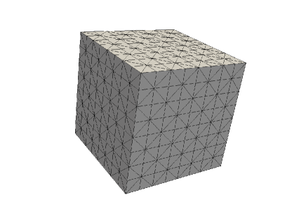
Figure 1: The initial mesh for Examples 4.1

The sequence of finite elements spaces are constructed by linear element on a series of meshes produced by regular refinement with $\beta=2$. In each level of the full multigrid scheme defined in Algorithm 3.2, the parameters are set to be $m=1$, $p=1$. And we take 3 conjugate gradient smooth steps for the presmoothing and postsmoothing iteration step in the multigrid iteration in the step 1 of Algorithm 3.1. Since the exact solution is not known, an adequate accurate approximation is chosen as the exact solution for our numerical test. Figure 1 shows the corresponding initial mesh.

Figure 2 gives the corresponding numerical results of Algorithm 3.2. From Figure 2, we can find that the full multigrid scheme can obtain the optimal error estimates for both eigenvalue and eigenvector.

In order to show the efficiency of Algorithm 3.2, we provide the CPU time for Algorithm 3.2. Here, we choose the Package ARPACK as the eigenvalue solving tool and the full multigrid scheme is running on the machine PowerEdge R720 with the linux system. The corresponding results are presented in Table 1 which shows the efficiency and linear complexity of Algorithm 3.2.

Table 1: The CPU time for Example 4.1 by Algorithm 3.2

Number of levels	Number of elements	Time for Algorithm 3.2
1	3072	0.45
2	24576	1.55
3	196608	8.08
4	1572846	63.01
5	12582912	519.86

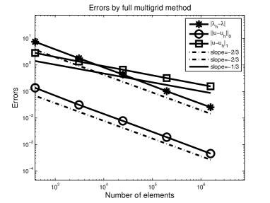
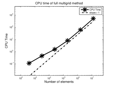
Figure 2: Left: The errors of the full multigrid method for the ground state solution of GPE, where $\lambda_{h}$ and $u_{h}$ denote the numerical eigenvalue and eigenfunction by Algorithm 3.2. Right: CPU Time of Algorithm 3.2 for Example 4.1

Example 4.2.

In the second example, we consider the GPE with the coefficient $\zeta=100$ and $W=x_{1}^{2}+x_{2}^{2}+x_{3}^{2}$ on the domain $\Omega=[0,1]^{3}$.

The initial mesh used in this example is the one shown in Figure 1. Numerical results are present in Table 2 and Figure 3. It is obvious, Table 2 and Figure 3 also show that the efficiency and linear complexity of Algorithm 3.2.

Table 2: The CPU time for Example 4.2 by Algorithm 3.2

Number of levels	Number of elements	time for Algorithm 3.2
1	24576	4.32
2	196608	11.43
3	1572846	70.88
4	12582912	577.52

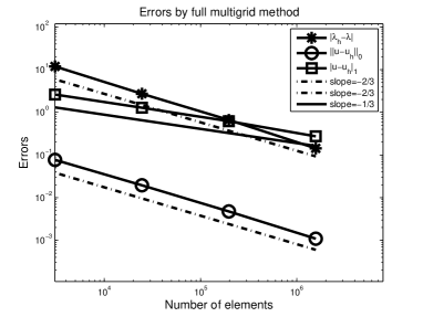
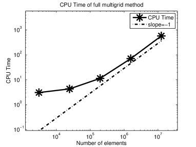
Figure 3: Left: The errors of the full multigrid method for the ground state solution of GPE, where $\lambda_{h}$ and $u_{h}$ denote the numerical eigenvalue and eigenfunction by Algorithm 3.2. Right: CPU Time of Algorithm 3.2 for Example 4.2

5 Concluding remarks

In this paper, a type of full multigrid method is introduced for nonlinear eigenvalue problems. The proposed methods is based on the combination of the multilevel correction technique for nonlinear eigenvalue problems and the multigrid iteration for linear boundary value problems. The multilevel correction technique can transform the nonlinear eigenvalue solving into a series of solutions of linear boundary value problems on a sequences of finite element spaces. The multigrid iteration is one of the efficient iteration which has uniform error reduction rate.

The multigrid iteration can also be replaced by other types of efficient iteration schemes such as algebraic multigrid method, the type of preconditioned schemes based on the subspace decomposition and subspace corrections (see, e.g., [9, 29]) and the domain decomposition method (see, e.g., [24, 30]).

References

• [1] R. A. Adams, Sobolev Spaces, Academic Press, New York, 1975.
• [2] R. E. Bank and T. Dupont, An optimal order process for solving finite element equations, Math. Comp., 36 (1981), 35-51.
• [3] W. Bao, The nonlinear Schr oinger equation and applications in Bose-Einstein condensation and plasma physics, Master Review, Lecture Note Series, Vol. 9, IMS, NUS, 2007.
• [4] W. Bao, Q. Du, Computing the ground state solution of Bose-Einstein condensates by a normalized gradient flow, SIAM J. Sci. Comput., 25 (2004), 1674-1697
• [5] J. H. Bramble, Multigrid Methods, Pitman Research Notes in Mathematics, Vol. 294, John Wiley and Sons, 1993.
• [6] J. H. Bramble and J. E. Pasciak, New convergence estimates for multigrid algorithms, Math. Comp., 49 (1987), 311-329.
• [7] J. H. Bramble and X. Zhang, The analysis of Multigrid Methods, Handbook of Numerical Analysis, Vol. VII, P. G. Ciarlet and J. L. Lions, eds., Elsevier Science, 173-415, 2000.
• [8] A. Brandt, S. McCormick, and J. Ruge, Multigrid methods for differential eigenproblems, SIAM J. Sci. Stat. Comput., 4(2) (1983), 244-260.
• [9] S. Brenner and L. Scott, The Mathematical Theory of Finite Element Methods, New York: Springer-Verlag, 1994.
• [10] E. Cancès, R. Chakir, Y. Maday, Numerical analysis of nonlinear eigenvalue problems, J. Sci. Comput., 45 (2010), 90-117.
• [11] H. Chen, X. Gong, L. He, Z. Yang and A. Zhou, Numerical analysis of finite dimensional approximations of Kohn-Sham models, Adv. Comput. Math., 38 (2013), 225-256.
• [12] H. Chen, X. Gong and A. Zhou, Numerical approximations of a nonlinear eigenvalue problem and applications to a density functional model, Math. Methods Applied Sci., 33 (2010), 1723-1742.
• [13] H. Chen, L. He and A. Zhou, Finite element approximations of nonlinear eigenvalue problems in quantum physics, Comput. Meth. Appl. Mech. Engrg., 200 (2011), 1846-1865.
• [14] P. G. Ciarlet, The finite Element Method for Elliptic Problem, North-holland Amsterdam, 1978.
• [15] W. Hackbusch, Multi-grid Methods and Applications, Springer-Verlag, Berlin, 1985.
• [16] W. Kohn and L. Sham, Self-consistent equations including exchange and correlation effects, Phys. Rev. A, 140 (1965), 4743-4754.
• [17] Q. Lin and H. Xie, A multi-level correction scheme for eigenvalue problems, Math. Comp., 84(291) (2015), 71-88.
• [18] R. Martin, Electronic Structure: Basic Theory and Practical Methods, Cambridge University Press, London, 2004.
• [19] S. F. McCormick, ed., Multigrid Methods. SIAM Frontiers in Applied Matmematics. Society for Industrial and Applied Mathematics, Philadelphia, 1987.
• [20] R. Parr and W. Yang, Density Functional Theory of Atoms and Molecules, Oxford University Press, New York, Clarendon Press, Oxford, 1994.
• [21] L. Scott and S. Zhang, Higher dimensional non-nested multigrid methods, Math. Comp., 58 (1992), 457-466.
• [22] V. Shaidurov, Multigrid methods for finite element, Kluwer Academic Publics, Netherlands, 1995.
• [23] C. Sulem and P. Sulem, The Nonlinear Schrödinger Equation: Self-focusing and Wave Collapse, Springer, New York, 1999.
• [24] A. Toselli and O. Widlund, Domain Decomposition Methods: Algorithm and Theory, Springer-Verlag, Berlin Heidelberg, 2005.
• [25] H. Xie, A type of multilevel method for the Steklov eigenvalue problem, IMA J. Numer. Anal., 34 (2014), 592-608.
• [26] H. Xie, A Type of Multi-level Correction Method for Eigenvalue Problems by Nonconforming Finite Element Methods, BIT Numerical Mathematics, doi:10.1007/s10543-015-0545-1, 1-24 (2015).
• [27] H. Xie, A multigrid method for eigenvalue problem, J. Comput. Phys., 274 (2014), 550-561.
• [28] H. Xie and M. Xie, A Multigrid Method for the Ground State Solution of Bose-Einstein Condensates, http://arxiv.org/abs/1408.6422, 2014.
• [29] J. Xu, Iterative methods by space decomposition and subspace correction, SIAM Review, 34(4) (1992), 581-613.
• [30] J. Xu and A. Zhou, Local and parallel finite element algorithm for eigenvalue problems, Acta Math. Appl. Sin. Engl. Ser., 18(2) (2002), 185-200.