Green thermoelectrics: Observation and analysis of plant thermoelectric response

Abstract

Plants are sensitive to thermal and electrical effects; yet the coupling of both, known as thermoelectricity, and its quantitative measurement in vegetal systems never were reported. We recorded the thermoelectric response of bean sprouts under various thermal conditions and stress. The obtained experimental data unambiguously demonstrate that a temperature difference between the roots and the leaves of a bean sprout induces a thermoelectric voltage between these two points. Basing our analysis of the data on the force-flux formalism of linear response theory, we found that the strength of the vegetal equivalent to the thermoelectric coupling is one order of magnitude larger than that in the best thermoelectric materials. Experimental data also show the importance of the thermal stress variation rate in the plant’s electrophysiological response. Therefore, thermoelectric effects are sufficiently important to partake in the complex and intertwined processes of energy and matter transport within plants.

I Introduction

Plants are complex biological systems, which feed, develop and function thanks to a variety of elementary and cooperative processes that ensure transport of energy and matter in the form of mineral elements, carbohydrates, and hormones in watery solutions called sap. Two categories of sap are transported in conductive tissues: xylem sap transported in xylem, a continuum of dead cells forming a pipe that opposes little resistance to the transport of water and mineral elements from roots to leaves; and phloem sap, containing water and sugar, formed in the leaves by photosynthesis, and transported in phloem (sieve tube elements) from the leaves to the roots. Explanations for xylem sap transport includes the cohesion-tension theory DixonJoly ; Askenasy and multiforce theories Tyree ; Zimmerman ; Wang ; and the pressure flow hypothesis proposes a mechanism for phloem sap transport DeSchepper2013 . Notwithstanding their relative merits, it is of interest to note that as saps contain ions, a net voltage may be recorded within plants. Furthermore, as a living plant is naturally submitted to a temperature gradient between its roots and its leaves, heat may also flow from its hotter to its colder regions. These two facts lead to the questions of the existence and strength of a coupling between electrical current and heat flux in plants, and whether this coupling plays a significant role in the plants’ lives. Answers to these questions are of importance to gain further insight into plant homeostasis, closely related to the Le Chatelier-Braun principle in chemical thermodynamics, and to develop further the field of plant electrophysiology by analysing the impact of thermoelectric coupling on photosynthesis, plant respiration, and any other processes involving bioelectrochemical phenomena PlantEP .

Biophysical processes, which include energy and matter transport in dedicated structures, are essentially nonequilibrium in nature. Their description involves the notions of thermodynamic forces and their conjugate fluxes which, in a linear response description, are proportional to each other. In a general manner, transport phenomena are nonequilibrium irreversible processesdeGroot ; Pottier2007 : fluxes within a system result from applied external constraints, and they are accompanied by energy dissipation and entropy production. As the forces applied to a system derive from potentials, the description of the system’s nonequilibrium properties relies on the definition of these potentials and their degree of coupling KedemCaplan . Thermoelectricity is sometimes mistakenly viewed as a phenomenon pertaining to solid-state systemsbookTE1 ; bookTE2 , but this effect has also been reported in liquidsLiquidThermoelec and gelsGelThermoelec . Now, considering more specifically electrical phenomena in plants, one should also account for their dependence on temperature and the local variations of this latter. As a matter of fact, one learns from the equilibrium thermodynamics of charged fluids that heat and electricity are fundamentally related through the Gibbs-Duhem relation; so, since plants, as any other system, are subjected to the laws of thermodynamics, one may anticipate that a proper understanding of the coupled transport of heat and electricity in plants will pave the way towards the potentially rich new field of thermoelectricity-based plant energy conversion, and harvesting metabolic energy from plants voltreepower .

Thermoelectricity as part of non-isothermal processes in living organisms, has already been mentioned; but except for the case of insects like hornets and bees Ishay ; Galushko ; Volynchik , for which genuine thermoeletric effects have been analysed, the other studies simply reported the record of the temperature rise of Colocasia odora leaves using a thermocouple VanBeek , or analysed pyroelectricity, mistakenly taken as a thermoelectricity, amongst the nonequilibrium processes at the origin of life Muller . We propose here to consider bean sprouts as an illustrative case of a living plant system whose physiological properties also entail thermoelectric effects, with a particular focus on the thermovoltage response of the plant. While a voltage difference along the stem of a plant has already been measured and analysed Love , its interpretation does not account for a likely the thermoelectric origin. Nevertheless, it is clear that the source of any voltage difference is due to concentration gradients of charges inside the plant, regardless of the cause of the gradients. The underlying processes may thus originate in various electrochemical processes, including acid-base and redox effectsLove . In the present work we focus on the voltage response due to a temperature difference. The system is presented in Fig. 1. The stem and leaves are kept at constant temperature while the temperature of the roots can be modified; the thermoelectric response is recorded on both the plant (a) and a control wire (b).

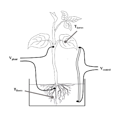
Figure 1: General view of the experimental setup. The voltage records are respectively on the plant (a), and the control wire (b).

II Theoretical considerations

Thermoelectricity differs from electrochemistry as the latter considers isothermal systems only. Thermoelectric effects, on the contrary, manifest themselves in non-isothermal conditions and their thermodynamic description is best done with the coupled variables $(\mu,T)$, where $\mu$ is the electrochemical potential and $T$ the temperature of the considered system. In a force-flux approach, as a temperature bias is applied to a conductor, both heat and charges are transported in coupled flows since each electron carries an electric charge, $e$, and energy; the thermoelectric coupling parameter or Seebeck coefficient $\alpha$ is thus defined as:

$$\alpha\overrightarrow{\nabla}T=-\frac{1}{e}\overrightarrow{\nabla}\mu$$ (1)

where $\overrightarrow{\nabla}$ denotes the spatial gradient. Equation (1) may be viewed as a generalization of the Gibbs-Duhem relation to the dynamical response of the coupled intensive variables $(\mu,T)$ by defining the thermodynamic forces acting on the system as the gradients of the thermodynamic potentials. Each force is conjugated to a flux which is proportional to the time derivative of the corresponding extensive parameter, and it follows that forces and fluxes are linearly combined as proposed by Onsager Onsager1 . Note that the coefficient $\alpha$, which in Eq. (1) is defined locally, is also often expressed as $\alpha\approx-e\Delta V/\Delta T$, where $\Delta$ denotes the global difference between two distant points of the system.

These general considerations apply for any system containing free charge carriers. As a consequence, for a given temperature difference, the measurement of a thermovoltage directly gives an estimation of the average ratio of charge concentrations in separate parts of the system. Therefore, any system containing free mobile carriers may be exhibit a thermoelectric signature. One should note that depending on the specific properties of the considered system, this signature may intertwine or not with those of other temperature-dependent processes; hence the need for specific system-dependent approaches to extract the thermoelectric signal. In the case of liquids and gels, the studies usually focus on the thermoelectrophoresis parameters LiquidThermoelec ; GelThermoelec ; Majee . For solid state-systems, the conduction is ensured by mobile electrons and holes, leading to a possible steady-state electrical current. For ionic carriers, in liquids and gels, such a steady-state current may only take place if a redox process occurs at the ends of the system.

III Experiment

The experiment aims to identify and characterize the thermoelectric response of a living plant (a bean sprout in the present work). As the response of the plant necessarily entails physiologic effects, the measured data is compared to the purely thermoelectric response of a control wire. As depicted on Fig. 1, the temperature of the plant’s roots is imposed by a thermostatic bath; two thermocouples are used to measure the temperatures of the roots and the leaves, and two electrodes are placed respectively in contact with the roots and the leaves of the living plant. The roots are bathed in an aqueous dilute KCl solution. The electrodes connected to the leaves are made of Ag/AgCl wires. All the temperatures and voltages are recorded using a Keithley K2700 scanning multimeter and a K182 nanovoltmeter. The thermoelectric control wire (CW) is made of two chromium-nickel-steel junctions, with a Seebeck coefficient $\alpha_{\rm junction}=4.6~{}\mu$V/K; it is placed in the same configuration as that of the plant. The recorded voltage at the ends of the control wire describes a pure thermoelectric response, exempt from any influence of the physiologic process.

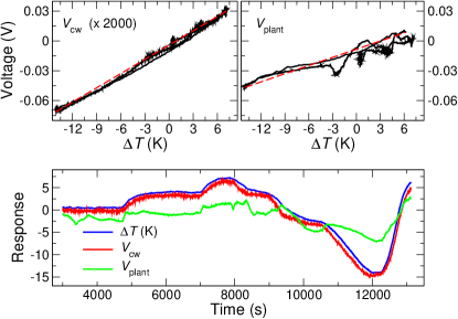
Figure 2: Experimental data including the voltage response of the control wire $V_{\rm cw}$ (upper left panel) and of the plant $V_{\rm plant}$ (upper right panel), both submitted to a time-varying temperature difference $\Delta T$, reported on the lower panel. The magnitude of measured voltage $V_{\rm cw}$ has been multiplied by a factor 2000 in order to report it on the same scale as that of $V_{\rm plant}$. The red-dotted lines indicate the average slope of the collected data. In the lower panel, the scale is that of the temperature difference; the voltages are also depicted in this lower panel to see how close their time-dependent behaviour is to that of the measured temperature difference.

The voltage response of the living plant and that of the control wire to the temperature difference $\Delta T$ are both shown on Fig. 2, where the time evolution of $\Delta T$ is also displayed, illustrating the dynamics of the plant and that of the control wire. These data were recorded over a period of four hours for various temperature differences and variation rates. The two upper panels show separately the parametric plots characterising the thermoelectric response of the control wire and that of the plant. Notice that the response of the control wire is strictly proportional to the temperature difference, as expected for a thermoelectric material, with a passive Seebeck coefficient. Conversely, the plant exhibits a complex response, which includes the effects of its physiological processes thus giving rise to an active Seebeck response. The curves represented on the lower panel are displayed together on the same scale to qualitatively show how the responses (voltages $V_{\rm cw}$ and $V_{\rm plant}$) follow the applied constraint (temperature difference $\Delta T$). The figures on the $y$-axis correspond to $\Delta T$ in ^∘C. The values taken by the voltages $V_{\rm cw}$ and $V_{\rm plant}$ may be determined from the curves using a scaling factor that corresponds to the relevant Seebeck coefficient. The control wire shows a faithful homothetic response to the temperature difference, with a linear factor of scaling of $4.6~{}\mu$V/K as expected for the Seebeck coefficient of the corresponding chromium-nickel-steel thermocouple. The response of the plant gives an average Seebeck coefficient of 2.5 mV/K. Such a large value in a solid-state material would correspond to a system with low electrical conductivity. Here, this results from ion movements through xylem and phloem saps circulating in opposite directions.

To analyze precisely these data, it is convenient to split each panel of Fig. 2 into three parts, which correspond to three distinct time domains. The first and third ones, Figs.3 and 5, respectively, describes the plant’s response when its roots are heated; while the second, Fig.4, reports the response over the cooling sequence.

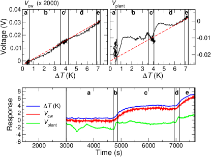
Figure 3: First heating sequence. The plant’s response is strongly influenced by the temperature variation rate ${\rm d}T/{\rm d}t$.

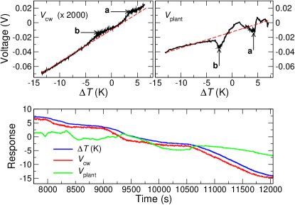
Figure 4: Cooling sequence. The response is roughly linear but visible discrepancies are due to the plant’s physiological processes.

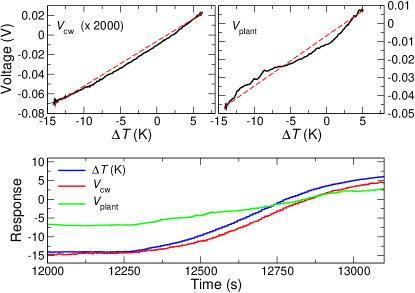
Figure 5: Second heating sequence.

Depending on the precise thermal condition supported by the plant, we can identify different thermoelectric responses. Consider the first warming sequence of Fig. 3. One may identify five events (labelled from a to e). During the first period (Fig. 3a), the temperature difference is roughly constant. The plant presents a large fluctuating thermoelectric response while the control wire is characterized by a constant Seebeck coefficient. During the second period, shown on Fig. 3b, the plant’s reaction is essentially sensitive to the temperature variation rate ${\rm d}T/{\rm d}t$. This sensitivity has already been observed in studies devoted to plant sensing Plieth1 ; Plieth2 . The processes taking place within the zones a and b can be also observed in the c and d zones; and when the rate ${\rm d}T/{\rm d}t$ is reduced, we observe a linear response for the plant, as shown in the zone e. It thus appears clearly that the passive response, probably mostly due to the xylem properties, can be strongly modified by active physiological processes. This latter appears to be particularly sensitive to the time derivative of the stress, but not so much on the intensity of the stress itself; this observation is perfectly consistent with previous findings Plieth1 ; Plieth2 .

We now turn to the cooling sequence, Fig. 4. The cooling rate is approximately constant, except for the two events when it is clearly larger than the average as indicated with the labels a and b, on the upper right panel. These events relate to time delays, also apparent in the measured data for the control wire on the upper left panel: these are signatures of the change of rate ${\rm d}T/{\rm d}t$. Note that although these may serve as a probe, time delays must be considered with care, since in the case of very large time response of a system, they may lead to erroneous interpretations GelThermoelec . The shape of the plant response for events taking place in the zones a and b is very similar to that of Figs. 3b and 3d, which confirms the acute sensitivity of the plant to the rate ${\rm d}T/{\rm d}t$. This physiological response is the fastest response to a stress that a plant can use, as it has no means to avoid it.

The last sequence depicted on Fig. 5 concerns the plant’s response to warming at a reduced rate. It is essentially linear, thus confirming the presence of a threshold rate process for the plant’s response to a given stress. It also shows unambiguously that thermoelectricity naturally partakes in the complex processes that contribute to a plant’s life.

IV Discussion and concluding remarks

All the effects discussed in the present work are related to the internal modifications of the ionic concentrations inside the plant, including the regulation of cellular ion transporters allowing ion release into the xylem sap toward the shoots. It is clear that while the response is mainly driven by a classical thermoelectric process with a giant Seebeck coefficient, the physiology of the plant interferes in a complex way with it. A complete numerical model, including series and parallel assemblies of living (phloem sieve tube elements, root and endodermis cells) and dead cells (xylem tracheids and vessels), will be considered for further investigation of the interplay between physiologic and thermoelectric response to a thermal stress. Further, since there is no limitation in the number of thermodynamic potentials which may be coupled Onsager1 , we may account for pressure and derive a complete response of a system to the direct and the cross- effects of the three thermodynamic potentials, $(P,\mu,T)$. Then the lowering of a local pressure gradient, by the coupled effect of the temperature and the electrochemical potential becomes possible. This latter process may contribute to the motion of saps in plant, and especially in trees.

The reported measurements are fully scalable from the unique cell size to a complete plant or tree. In addition to the stationary response observed here, the voltage fluctuations are also of great interest since they permit the study of the threshold of the physiological response through its noisy signals. As observed in other systems, the noise response is a very sensitive probe of the emergence of a macroscopic response noise1 ; noise2 . Taking each cell as a fluctuator, the convolution of the individual responses may lead to different signatures depending on the considered scale of the sample.

Appendix A Plant material

Seeds of bush bean (Phaseolus vulgaris L. cv. contender) were sown into pots containing vermiculite as soil. The bean seedlings were grown in a growth chamber at $25\pm 2^{\circ}$C with a cycle of 12 hours of light (40 $\mu$mol photon m${}^{-2}\cdot$ s^-1), 12 hours of darkness. The plants were watered at the bottom of the pots every three days. The 21 days old plants were removed from the vermiculite. Roots were carefully rinsed with water to remove vermiculite particles and then transferred in dilute KCl solution (120 mM) for experiments.

Appendix B Measurement electrodes

Two electrodes were placed respectively at the surface of the root and the stem of the living plant. The electrodes connected to the stems are made of Ag/AgCl wires moistened with 200 mM KCl and wrapped in cellophane to provide appropriate contact with the plant surface.

References

- (1) H. H. Dixon and J. Joly, Ann. Bot. 8, 468 (1894).
- (2) E. Askenasy, Bot. Cent. 62, 237 (1895).
- (3) M. T. Tyree, J. Exp. Bot. 48, 1753 (1997).
- (4) U. Zimmerman et al., Physiol. Plant. 114, 327 (2002).
- (5) Z. Wang, C. C. Chang, S. J. Hong, Y. J. Sheng, and H.-K. Tsao, Langmuir 28, 16917 (2012).
- (6) V. De Schepper, T De Swaef., I. Bauweraerts, and K. Steppe, J. Exp. Bot. 64, 4839-4850 (2013).
- (7) A. G. Volkov, Ed., Plant Electrophysiology: Theory and Methods, (Springer Berlin Heidelberg, 2006).
- (8) S. R. de Groot, Thermodynamics of Irreversible Processes (Intersciences Publishers Inc., New York, 1958).
- (9) N. Pottier, Non-equilibrium Statistical Physics (Oxford University Press, Oxford, 2010).
- (10) O. Kedem and S. R. Caplan, Trans. Faraday Soc. 61, 1897 (1965).
- (11) D. M. Rowe, Ed. CRC Handbook of Thermoelectrics (CRC Press LLC, Boca Raton, 2010).
- (12) K. Koumoto and T. Mori, Eds., Thermoelectric Nanomaterials (Springer Series in Materials Science, Vol. 182, Springer, Berlin Heidelberg, 2013).
- (13) H. Liu et al. Copper ion liquid-like thermoelectrics. Nature Mater. 11, 422 (2012).
- (14) B. R. Brown, M. E. Hughes, and C. Russo, Phys. Rev. E 70, 031917 (2004).
- (15) Voltree Power, http://voltreepower.com/ (2014).
- (16) J. S. Ishay, V. Pertsis, E. Rave, A. Goren, and D. J. Bergman, Phys. Rev. Lett. 90, 218102 (2003).
- (17) D. Galushko et al., Semicond. Sci. Technol. 20, 286 (2005).
- (18) S. Volynchik, M. Plotkin, N. Y. Ermakov, D. J. Bergman, and J. S. Ishay, Microsc. Res. and Tech. 69, 903 (2006).
- (19) A. Van Beek and C. A. Bergsma, Observations thermo-électriques sur l’élévation de température des fleurs de Colocasia odora (Robert Natan, Utrecht, 1838).
- (20) A. W. J. Muller, Phys. Letter A 96, 319 (1985).
- (21) C. J. Love, S. Zhang, and A. Mershin, PLoS ONE 3 (8): e2963 (2008). DOI: 10.1371/journal.pone.0002963
- (22) H. B. Callen, Phys. Rev. 73, 1349 (1948).
- (23) L. Onsager, Phys. Rev. 37, 405 (1931).
- (24) A. Majee and A. Wurger, Phys. Rev. E 83, 061403 (2011).
- (25) C. Plieth, U. P. Hansen, H. Knight, and M. R. Knight, TPlant J. 18, 491 (1999).
- (26) C. Plieth, J. Membrane Biol. 172, 121 (1999).
- (27) J. Scola, A. Pautrat, C. Goupil, Ch. Simon, B. Domengès, and C. Villard, Fluct. Noise Lett. 6, L287 (2006).
- (28) O. Ben-David, S. M. Rubinstein, and J. Fineberg, Nature 463, 76 (2010).