Leader-follower Tracking Control with Guaranteed Consensus Performance for Interconnected Systems with Linear Dynamic Uncertain Coupling 

Abstract

This paper considers the leader-follower tracking control problem for linear interconnected systems with undirected topology and linear dynamic coupling. Interactions between the systems are treated as linear dynamic uncertainty and are described in terms of integral quadratic constraints (IQCs). A consensus-type tracking control protocol is proposed for each system based on its state relative its neighbors. In addition a selected set of subsystems uses for control their relative states with respect to the leader. Two methods are proposed for the design of this control protocol. One method uses a coordinate transformation to recast the protocol design problem as a decentralized robust control problem for an auxiliary interconnected large scale system. Another method is direct, it does not employ coordinate transformation; it also allows for more general linear uncertain interactions. Using these methods, sufficient conditions are obtained which guarantee that the system tracks the leader. These conditions guarantee a suboptimal bound on the system consensus and tracking performance. The proposed methods are compared using a simulation example, and their effectiveness is discussed. Also, algorithms are proposed for computing suboptimal controllers.

Keywords: Large-scale systems, robust distributed control, leader-follower tracking control, consensus control, integral quadratic constraints.

1 Introduction

Theoretical study of distributed coordination and control has received increasing attention in the past decade, due to its broad applications in unmanned air vehicles (UAVs) (Beard et al., 2002), formation control (Fax & Murray, 2004), flocking (Olfati-Saber, 2006) and distributed sensor networks (Cortes & Bullo, 2003), etc. As a result, much progress has been made in the study of cooperative control of complex systems (Olfati-Saber, Fax, & Murray, 2007; Ren, Beard, & Atkins, 2007), with the aim to develop feedback control tools to achieve a desired system behavior. In particular, synchronization problems for interconnected networks of complex dynamical systems are actively studied (Arenas et al., 2008; Tuna, 2008, 2009).

There exist a number of approaches to achieve synchronized behavior in systems comprised of many dynamic subsystems-agents. These approaches include the average consensus approach (Olfati-Saber, Fax, & Murray, 2007), the approach based on internal model principle (Wieland, Sepulchre, & Allgöwer, 2011), and the leader-follower approach. In the latter approach, one of the agents is designated to serve as a leader, and interconnections within the system are designed to let the rest of the system follow the leader (Pecora & Carroll, 1990; Grip, Yang, Saberi, & Stoorvogel, 2012). This approach, known as leader-follower approach, is the main focus of this paper.

The majority of leader-follower problems considered in the literature assume that dynamics of the agents are dynamically decoupled (Jadbabaie, Lin, & Morse, 2003; Hong, Hu, & Gao, 2006; Zhao, Li, & Duan, 2013), and the information flow between the subsystems is directed (Ren & Atkins, 2007) and is used for control. While these assumptions are justifiable in the case of multi-agent systems such as autonomous vehicle formations, in many physical systems, interactions are unavoidable and have undirected nature (Šiljak, 1978; Šiljak & Zecevic, 2005). The Newtonian interaction between mechanical systems (e.g., the gravitational attraction between satellites), and the Coulomb forces between charged particles are the examples of such undirected interactions. Moreover, implementation of control protocols using these physical principles (e.g., by interconnecting physical masses with springs and dampers) inevitably leads to undirected control interactions. Hence, there is a need to explore situations where undirected interactions occur at both interconnection and control level (Persis, Sailer, & Wirth, 2013). This motivates us to consider undirected control schemes.

Compared with the existing work in the field of the leader-follower tracking consensus problem, we consider a quite general class of physical interactions between subsystems. These interactions include both static and dynamic interactions, such as unmodelled linear dynamics, uncertain input delays and norm-bounded uncertainties. To capture such a broad class of interactions, we regard them as an uncertainty and describe them in terms of time-domain integral quadratic inequalities known as Integral Quadratic Constraints (IQCs) (Petersen, Ugrinovskii, & Savkin, 2000; Megretski & Rantzer, 1997). The IQC modeling is a well established technique to describe uncertain interactions between subsystems in a large scale system. It has led to a number of solutions to optimal and suboptimal decentralized control problems (Ugrinovskii & Pota, 2005; Li, Ugrinovskii, & Orsi, 2007; Ugrinovskii et al., 2000).

As in these references, the IQC modelling allows us to account for the effects of interconnections between subsystems from a robustness viewpoint. However, different from the above references, the IQC methodology is developed here for the design of distributed consensus-type feedback tracking controllers.

In the context of robust consensus analysis, the recent paper (Trentelman, Takaba, & Monshizadeh, 2013) is worth mentioning, which considers robust consensus protocols for synchronization of multi-agent systems under additive uncertain perturbations with bounded $H_{\infty}$ norm. Since the IQC conditions in our paper capture uncertain perturbations with bounded $L_{2}$ gain, we note a similarity between the two uncertainty classes. However, thanks to the time-domain IQC modelling, our paper goes beyond the analysis of robust consensus. It develops the technique for leader-follower distributed tracking control synthesis, which provides an optimized guarantee of performance of the leader-follower tracking system under consideration (note also that Trentelman, Takaba, & Monshizadeh (2013) consider a leaderless network).

The key element of our approach to the leader-follower tracking control synthesis is an optimization formulation which imposes a cost on the worst-case consensus tracking performance of the system, as well as on protocol actions. This approach is inspired by the recent results on distributed LQR design (Borrelli & Keviczky, 2008; Zhang, Lewis, & Das, 2011; Zhao, Duan, Wen & Chen, 2012). It allows us to recast the original consensus tracking problem as a decentralized guaranteed cost control problem for a certain auxiliary large-scale system. This leads to a distributed control design method for the system of coupled subsystems, where local tuning parameters can be chosen to minimize the bound on the consensus performance of the protocol leading to a suboptimal guaranteed performance. This reduces the original problem to an optimization problem involving coupled parameterized linear matrix inequalities (LMIs). We also show that the design of the tracking protocol can be simplified using decoupled LMIs. This however leads to a weaker tracking result in that we can only guarantee a greater bound on consensus tracking performance. Furthermore, we compare this method with an alternative method based on direct overbounding of the original performance cost. The advantage of this method is that it can be extended to the case of interconnected systems with more general linear uncertain dynamic coupling, as demonstrated in Section 3.4.

The main contributions of the paper are sufficient conditions for the design of a guaranteed consensus tracking performance protocol for interconnected systems subject to linear dynamic IQC-constrained coupling. To derive such conditions, we first transform the underlying guaranteed consensus performance control problem into a guaranteed cost decentralized robust control for an auxiliary large scale system, which is comprised of coupled subsystems. The interconnections pose an additional difficulty here, compared with recent results, e.g., Li, Duan, Chen, & Huang (2010); Zhang, Lewis, & Das (2011), where similar transformations resulted in a set of completely decoupled stabilization problems. To overcome the effect of the interconnections, we employ the minimax control design methodology of decentralized control synthesis (Ugrinovskii & Pota, 2005; Li, Ugrinovskii, & Orsi, 2007; Ugrinovskii et al., 2000). We then discuss an alternative sufficient condition whose derivation does not involve the coordinate transformation. We show using an example that our main result may offer an advantage, compared with this alternative condition. Finally, the computational algorithms are introduced to optimize the proposed guaranteed bounds on the consensus tracking performance.

The preliminary version of the paper was presented at the 2013 American Control Conference (Cheng & Ugrinovskii, 2013). Compared to Cheng & Ugrinovskii (2013), this paper has been substantially extended. Firstly, in this paper, more general linear uncertain coupling is considered, and the leader is allowed to dynamically couple with some of the followers. In addition, we present a detailed comparison of the results in Cheng & Ugrinovskii (2013) with those obtained using a direct technique which does not involve coordinate transformation. Another extension in this paper is concerned with the computational algorithms, which demonstrate how the design of a suboptimal tracking protocol can be carried out by minimizing the proposed guaranteed bound on the consensus tracking performance.

The paper is organized as follows. Section 2 includes the problem formulation and some preliminaries. The main results are given in Section 3. In Section 4, the computational algorithms are introduced. Section 5 provides the illustrative example. The conclusions are given in Section 6. All the proofs are given in the Appendix.

2 Problem Formulation and Preliminaries

2.1 Interconnection and communication graphs

Unlike many papers that study the leader-follower tracking problem for decoupled systems (cf. Hong, Hu, & Gao (2006); Ren & Atkins (2007)), we draw a distinction between the network representing ’physical’ interactions (including the leader) and the network that realizes ’control’ interactions. The rationale for considering the two-network structure is twofold. Firstly, synchronization protocols must be designed for followers only, and should have no direct impact on the leader. Also, the control interactions do not have to replicate the topology of physical interconnections.

Consider an undirected interconnection graph $\mathcal{G}=(\mathcal{V},\mathcal{E}^{\phi},\mathcal{A}^{\phi})$, where $\mathcal{V}=\{0,\ldots,N\}$ is a finite nonempty node set and $\mathcal{E}^{\phi}\subseteq\mathcal{V}\times\mathcal{V}$ is an edge set of unordered pairs of nodes. Without loss of generality, the node $0$ will be assigned to represent the leader, while the nodes from the set $\mathcal{V}_{0}=\{1,\ldots,N\}$ will represent the followers. The coupling between the followers is described by a subgraph $\mathcal{G}_{0}$ of $\mathcal{G}$ defined on the node set $\mathcal{V}_{0}$ with the edge set $\mathcal{E}_{0}^{\phi}\subseteq\mathcal{V}_{0}\times\mathcal{V}_{0}$. The edge $(i,j)$ in the edge sets $\mathcal{E}^{\phi}$, $\mathcal{E}_{0}^{\phi}$ means that nodes $i$ and $j$ influence each other through physical interconnections.

Let $\mathcal{A}^{\phi}_{0}$ be the adjacency matrix of the subgraph $\mathcal{G}_{0}$; $a_{ij}^{\phi}$ are the elements of its $i$th row where $a_{ij}^{\phi}=1$ if $(i,j)\in\mathcal{E}_{0}^{\phi}$, and $a_{ij}^{\phi}=0$ otherwise. The Laplacian matrix of the subgraph $\mathcal{G}_{0}$ is defined as $\mathcal{L}^{\phi}_{0}=\mathcal{F}-\mathcal{A}^{\phi}_{0}$, where $\mathcal{F}=\mathrm{diag}\{f_{1},\ldots,f_{N}\}\in R^{N\times N}$ is the in-degree matrix of $\mathcal{G}_{0}$, i.e., the diagonal matrix, whose diagonal elements are the in-degrees of the corresponding nodes of the graph $\mathcal{G}_{0}$, $f_{i}=\sum_{j=1}^{N}a_{ij}^{\phi}$ for $i=1,\ldots,N$. In accordance with this structure, the adjacency matrix $\mathcal{A}^{\phi}$ of the undirected graph $\mathcal{G}$ is obtained by augmenting $\mathcal{A}^{\phi}_{0}$ as follows

$$\mathcal{A}^{\phi}=\left[\begin{array}[]{c|c}0&d^{\prime}\\ \hline\cr d&\mathcal{A}^{\phi}_{0}\end{array}\right],$$

where $d=[d_{1}\leavevmode\nobreak\ \ldots\leavevmode\nobreak\ d_{N}]^{\prime}$, with $d_{i}=1$ if there is the interconnection between the $i$th follower and the leader, and $d_{i}=0$ otherwise.

Also, consider an undirected control graph $\mathcal{C}=(\mathcal{V}_{0},\mathcal{E}^{c},\mathcal{A}^{c})$ with the same vertex set $\mathcal{V}_{0}$ and an undirected edge set $\mathcal{E}^{c}\subseteq\mathcal{V}_{0}\times\mathcal{V}_{0}$. An unordered pair $(i,j)$ in the edge set $\mathcal{E}^{c}$ indicates that nodes $i$ and $j$ obtain information from each other, which they will use for control. $\mathcal{C}$ is assumed to have no self-loops or repeated edges. The adjacency matrix $\mathcal{A}^{c}=[a_{ij}^{c}]\in R^{N\times N}$ of the undirected graph $\mathcal{C}$ is defined as $a_{ij}^{c}=a_{ji}^{c}=1$ if $(i,j)\in\mathcal{E}^{c}$, and $a_{ij}^{c}=a_{ji}^{c}=0$ otherwise. The degree matrix $\mathcal{H}=\mathrm{diag}\{h_{1},\ldots,h_{N}\}\in R^{N\times N}$ is a diagonal matrix, whose diagonal elements are $h_{i}=\sum_{j=1}^{N}a_{ij}^{c}$ for $i=1,\ldots,N$. The Laplacian matrix of this graph is denoted as $\mathcal{L}^{c}=\mathcal{H}-\mathcal{A}^{c}.$ It is symmetric since $\mathcal{C}$ is undirected.

We assume throughout the paper that the leader is observed by a subset of followers. If the leader is observed by follower $i$, we extend the graph $\mathcal{C}$ by adding the directed edge $(i,0)$, and assign this edge with the weighting $g_{i}=1$, otherwise we let $g_{i}=0$. We refer to node $i$ with $g_{i}\neq 0$ as a pinned or controlled node. Denote the pinning matrix as $G=\mathrm{diag}\left[g_{1},\ldots,g_{N}\right]\in\Re^{N\times N}$. The system is assumed to have at least one follower which can observe the leader, hence $G\neq 0$. The extended graph represents the communication topology for control and is denoted as $\hat{\mathcal{C}}$. Let $g=[g_{1}\leavevmode\nobreak\ \ldots\leavevmode\nobreak\ g_{N}]^{\prime}$, its adjacency matrix $\hat{\mathcal{A}}^{c}$ is defined as

$$\hat{\mathcal{A}}^{c}=\left[\begin{array}[]{c|c}0&0\\ \hline\cr g&\mathcal{A}^{c}\end{array}\right].$$

Finally, we introduce the notation for neighborhoods in the above graphs. Node $j$ is called a neighbor of node $i$ in the graph $\mathcal{C}$ ($\mathcal{G}$ or $\mathcal{G}_{0}$, respectively) if $(i,j)\in\mathcal{E}^{c}$ ($\mathcal{E}^{\phi}$ or $\mathcal{E}_{0}^{\phi}$, respectively). The sets of neighbors of node $i$ in the graphs $\mathcal{C}$, $\mathcal{G}$ and $\mathcal{G}_{0}$ are denoted as $S^{c}_{i}=\{j|(i,j)\in\mathcal{E}^{c}\}$, $S^{\phi}_{i}=\{j|(i,j)\in\mathcal{E}^{\phi}\}$, and $S_{i}=\{j|(i,j)\in\mathcal{E}_{0}^{\phi}\}$, respectively.

2.2 Problem Formulation

Consider a system consisting of $N+1$ interconnected subsystems; these interconnections are described by the undirected graph $\mathcal{G}$. Dynamics of the $i$th subsystem are described by the equation

$$\dot{x}_{i}=Ax_{i}+B_{1}u_{i}+B_{2}\sum\limits_{j\in S_{i}^{\phi}}\varphi(t,x_{j}(.)|_{0}^{t}-x_{i}(.)|_{0}^{t}),$$ (1)

where the notation $\varphi(t,y(.)|_{0}^{t})$ describes an operator mapping functions $y(s)$, $0\leq s\leq t$, into $\Re^{m}$. Also, $x_{i}\in\Re^{n}$ is the state, $u_{i}\in\Re^{p}$ is the control input. We note that the last term in (1) reflects a relative, time-varying nature of interactions between the subsystems.

Let $L_{2e}^{n}[0,\infty)$ be the space of functions $y(.):[0,\infty)\rightarrow\Re^{n}$ such that $\int_{0}^{t}\|y(t)\|^{2}dt<\infty,\leavevmode\nobreak\ \forall t>0$.

Assumption 1

Given a matrix $C\in\Re^{r\times n}$, the mapping $\varphi(.,.)$ satisfies the following assumptions:

1. $\forall y\in L_{2e}^{n}[0,\infty)$, $\varphi(.,y(.)|_{0}^{.})\in L_{2e}^{m}[0,\infty)$.

2. $\forall t>0$, $\varphi(t,y)$ is linear in the second argument; i.e., if $y=\alpha_{1}y_{1}+\alpha_{2}y_{2}$, then $\varphi(t,y(.)|_{0}^{t})=\alpha_{1}\varphi(t,y_{1}(.)|_{0}^{t})+\alpha_{2}\varphi(t,y_{2}(.)|_{0}^{t})$.

3. There exists a sequence $\{t_{l}\}$, $t_{l}\rightarrow\infty$, such that for every $t_{l}$, the following IQC holds

   $$\int_{0}^{t_{l}}\|\varphi(t,y(.)|_{0}^{t})\|^{2}dt\leq\int_{0}^{t_{l}}\|Cy\|^{2}dt,\quad\forall y\in L_{2e}[0,\infty).$$ (2)

The class of such operators will be denoted by $\Xi_{0}$.

Remark 1

Assumption 1 captures some common classes of uncertain coupling. For example, $\varphi$ can be a linear causal operator from the Hardy space $H_{\infty}$. Such operators have extension to operators mapping $L_{2e}[0,\infty)$ into $L_{2e}[0,\infty)$ (Willems, 1971). For instance, it is easy to show that unmodelled dynamics described as

$$\left\{\begin{array}[]{ll}\dot{\zeta}_{i}=-a_{i}{\zeta}_{i}+y(t),\leavevmode\nobreak\ \leavevmode\nobreak\ \zeta_{i}(0)=0,\\ \varphi(t,y(.)|_{0}^{t})=\zeta_{i}(t),\end{array}\right.$$

satisfy (2). Then the term $\varphi(t,x_{j}(.)-x_{i}(.))$ in (1) reduces to $\varphi(x_{j}(.)-x_{i}(.))$ and can be interpreted as an action based on relative measurements and applied through a stationary dynamic channel with memory. Uncertain input delay in receiving relative states is also allowed by this assumption, which can be described by choosing

$$\varphi(t,y(.)|_{0}^{t})=\begin{cases}Cy(t-\tau),\leavevmode\nobreak\ t\geq\tau,\\ 0,\leavevmode\nobreak\ 0\leq t<\tau,\end{cases}$$

where $\tau$ is uncertain delay parameter. For this $\varphi$ we have

$$\int_{0}^{t_{l}}\|\varphi(t,y(.)|_{0}^{t})\|^{2}dt=\int_{0}^{t_{l}-\tau}\|Cy(s)\|^{2}ds\leq\int_{0}^{t_{l}}\|Cy(s)\|^{2}ds.$$

This implies that uncertain input delay in receiving relative states is allowed by Assumption 1.

Finally, (2) captures norm-bounded uncertain coupling by allowing the uncertainty of the form $\varphi(t,y(.)|_{0}^{t})=\Delta(t)y(t)$ where ${\Delta}$ is a time varying matrix such that ${\Delta^{\prime}(t)}\Delta(t)\leq C^{\prime}C$.

Since we have designated node $0$ to be the leader, the leader is not controlled, i.e., $u_{0}\equiv 0$. On the contrary, all other follower nodes will be controlled to track the dynamics of the leader node. In this paper we are concerned with finding a control protocol for each follower node $i$, of the form

$$u_{i}=-K\{\sum\limits_{j\in S^{c}_{i}}(x_{j}-x_{i})+g_{i}(x_{0}-x_{i})\},$$ (3)

where $K\in\Re^{p\times n}$ is the feedback gain matrix to be found.

As a measure of the system performance, we will use the quadratic cost function (cf. Borrelli & Keviczky (2008)),

$$\mathcal{J}(u)=\sum\limits_{i=1}^{N}\int_{0}^{\infty}\Big{(}\frac{1}{2}\sum\limits_{j\in S^{c}_{i}}(x_{j}-x_{i})^{\prime}Q(x_{j}-x_{i})+g_{i}(x_{0}-x_{i})^{\prime}Q(x_{0}-x_{i})+u_{i}^{\prime}Ru_{i}\Big{)}dt,$$ (4)

where $Q=Q^{\prime}>0$ and $R=R^{\prime}>0$ are given weighting matrices, $u$ denotes the vector $u=[u_{1}^{\prime}\leavevmode\nobreak\ \ldots\leavevmode\nobreak\ u_{N}^{\prime}]^{\prime}$. The cost function (4) penalizes the system inputs. It also penalizes the disagreement between subsystems and their neighbors as well as the tracking error between the leader and the pinned subsystems which observe the leader.

The problem in this paper is to find a control protocol (3) which solves the following guaranteed consensus performance tracking problem:

Problem 1

Under Assumption 1, find a control protocol of the form (3) such that

$$\sup\limits_{\Xi_{0}}\mathcal{J}(u)<\infty.$$ (5)

It will be shown later that (5) implies $e_{i}\in L_{2}[0,\infty)$ $\forall i=1,\ldots,N$, where $e_{i}=x_{0}-x_{i}$ is the tracking error at node $i$. Hence, solving Problem 1 will guarantee that all followers synchronize to the leader in the $L_{2}$ sense.

2.3 Associated Decentralized Guaranteed Cost Control Problem

In this section, we introduce an auxiliary decentralized guaranteed cost control problem for an interconnected large scale system. Our approach follows (Li, Duan, Chen, & Huang, 2010; Zhang, Lewis, & Das, 2011), however here it results in a collection of coupled subsystems.

From (1) and taking the linearity of the operator $\varphi$ into account, dynamics of the tracking error vectors satisfy the equation

$$\dot{e}_{i}=Ae_{i}-B_{1}u_{i}-B_{2}\sum\limits_{j\in S_{i}}(\varphi(t,e_{i}(.)|_{0}^{t})-\varphi(t,e_{j}(.)|_{0}^{t}))-B_{2}\sum\limits_{k\colon d_{k}=1}\varphi(t,e_{k}(.)|_{0}^{t})-B_{2}d_{i}\varphi(t,e_{i}(.)|_{0}^{t}).$$ (6)

Then the closed loop system consisting of the error dynamics (6) and the protocol (3) can be represented as

$$\dot{e}=(I_{N}\otimes A)e+((\mathcal{L}^{c}+G)\otimes(B_{1}K))e-((\mathcal{L}_{0}^{\phi}+D+\bar{D})\otimes B_{2})\Phi(t),$$ (7)

where $\otimes$ denotes the Kronecker product, and $e=[e_{1}^{\prime}\leavevmode\nobreak\ \ldots\leavevmode\nobreak\ e_{N}^{\prime}]^{\prime}$, $D=\mathrm{diag}[d_{1},\ldots,d_{N}]$,

$$\bar{D}=\left[\begin{array}[]{cccc}d_{1}&d_{2}&\cdots&d_{N}\\ d_{1}&d_{2}&\cdots&d_{N}\\ \vdots&\vdots&&\vdots\\ d_{1}&d_{2}&\cdots&d_{N}\end{array}\right],\quad\Phi(t)=\left[\begin{array}[]{c}\varphi(t,e_{1}(.)|_{0}^{t})\\ \varphi(t,e_{2}(.)|_{0}^{t})\\ \vdots\\ \varphi(t,e_{N}(.)|_{0}^{t})\end{array}\right].$$

It was shown in Hong, Hu, & Gao (2006) that if the communication graph $\mathcal{C}$ is connected and at least one agent can observe the leader, then the symmetric matrix $\mathcal{L}^{c}+G$ is positive definite, Hence all its eigenvalues are positive. Let $T\in\Re^{N\times N}$ be an orthogonal matrix such that

$$T^{-1}(\mathcal{L}^{c}+G)T=J=\mathrm{diag}\left[\lambda_{1},\ldots,\lambda_{N}\right].$$ (8)

Also, let $\varepsilon=(T^{-1}\otimes I_{n})e$, $\varepsilon=[\varepsilon_{1}^{\prime}\leavevmode\nobreak\ \ldots\leavevmode\nobreak\ \varepsilon_{N}^{\prime}]^{\prime}$ and $\Psi(t)=(T^{-1}\otimes I_{m})\Phi(t)$. Using this coordinate transformation, the system (7) can be represented in terms of $\varepsilon$, as

$$\begin{split}\dot{\varepsilon}=&\big{(}{I_{N}\otimes A+J\otimes(B_{1}K)}\big{)}\varepsilon-\big{(}M\otimes B_{2}\big{)}\Psi(t),\end{split}$$ (9)

where $M=T^{-1}(\mathcal{L}_{0}^{\phi}+D+\bar{D})T$ and

$$\Psi(t)=\left[\begin{array}[]{ccc}\varphi(t,\sum\limits_{j=1}^{N}(T^{-1})_{1j}e_{j}(.)|_{0}^{t})\\ \vdots\\ \varphi(t,\sum\limits_{j=1}^{N}(T^{-1})_{Nj}e_{j}(.)|_{0}^{t})\end{array}\right]=\left[\begin{array}[]{ccc}\varphi(t,\varepsilon_{1}(.)|_{0}^{t})\\ \vdots\\ \varphi(t,\varepsilon_{N}(.)|_{0}^{t})\end{array}\right].$$

Here we used the assumption that $\varphi(t,\cdot)$ is a linear operator. It follows from (9) that the system (9) can be regarded as a closed loop system consisting of $N$ interconnected linear uncertain subsystems of the following form

$$\dot{\varepsilon}_{i}=A\varepsilon_{i}+B_{1i}\hat{u}_{i}+E_{i}\xi_{i}+L_{i}\eta_{i},$$ (10)

each governed by a state feedback controller $\hat{u}_{i}=K\varepsilon_{i}$. Here we have used the following notation

$$\xi_{i} =\varphi(t,\varepsilon_{i}(.)|_{0}^{t}),$$ (11)

$$\eta_{i} =[\xi_{1}^{\prime}\leavevmode\nobreak\ \ldots\leavevmode\nobreak\ \xi_{i-1}^{\prime}\leavevmode\nobreak\ \xi_{i+1}^{\prime}\leavevmode\nobreak\ \ldots\leavevmode\nobreak\ \xi_{N}^{\prime}]^{\prime},$$ (12)

$$B_{1i} ={\lambda}_{i}B_{1},$$

$$E_{i} =-M_{i,i}B_{2},$$

$$L_{i} =-B_{2}[M_{i,1}I,\ldots,M_{i,(i-1)}I,M_{i,(i+1)}I,\ldots,M_{i,N}I].$$

From Assumption 1, the following two inequalities hold for all $i=1,\ldots,N$:

$$\int_{0}^{t_{l}}\|\xi_{i}\|^{2}dt\leq\int_{0}^{t_{l}}\|C\varepsilon_{i}\|^{2}dt,$$ (13)

$$\int_{0}^{t_{l}}\|\eta_{i}\|^{2}dt\leq\int_{0}^{t_{l}}\sum\limits_{j\neq i}\|C\varepsilon_{j}\|^{2}dt.$$ (14)

It follows from (13) and (14) that the collection of uncertainty inputs $\xi_{i}$, $\eta_{i}$, $i=1,\ldots,N$, represents an admissible local uncertainty and admissible interconnection inputs for the large-scale system (10), respectively; see Petersen, Ugrinovskii, & Savkin (2000); Ugrinovskii & Pota (2005); Li, Ugrinovskii, & Orsi (2007); Ugrinovskii et al. (2000). Let $\Xi$, $\Pi$ be the sets of all uncertainty inputs and admissible interconnection inputs for the system (10) for which conditions (13) and (14) hold. Thus, we conclude that if $\varphi$ satisfies the conditions in Assumption 1, then the corresponding signals (11), (12) belong to $\Xi$, $\Pi$, respectively.

Next, consider the performance cost (4). It is possible to show that

$$\mathcal{J}(u)=\int_{0}^{\infty}\Big{(}e^{\prime}((\mathcal{L}^{c}+G)\otimes Q)e+{u}^{\prime}(I\otimes R){u}\Big{)}dt.$$ (15)

Since $T$ is an orthogonal matrix and $\varepsilon=(T^{-1}\otimes I_{n})e$, then $e=(T\otimes I_{n})\varepsilon$ and

$$u=-\big{[}\big{(}(\mathcal{L}^{c}+G)T\big{)}\otimes K\big{]}\varepsilon.$$

Since $T^{\prime}T=TT^{\prime}=I_{N}$, this allows the performance cost to be expressed as

$$\mathcal{J}(u) =\int_{0}^{\infty}\Big{(}\varepsilon^{\prime}\Big{(}\big{(}T^{\prime}(\mathcal{L}^{c}+G)T\big{)}\otimes Q\Big{)}\varepsilon+\varepsilon^{\prime}\Big{(}\big{(}T^{\prime}(\mathcal{L}^{c}+G)(\mathcal{L}^{c}+G)T\big{)}\otimes(K^{\prime}RK)\Big{)}\varepsilon\Big{)}dt$$

$$=\sum_{i=1}^{N}\int_{0}^{\infty}\big{(}\lambda_{i}\varepsilon_{i}^{\prime}Q\varepsilon_{i}+\lambda_{i}^{2}{\varepsilon}_{i}^{\prime}K^{\prime}RK{\varepsilon_{i}}\big{)}dt.$$ (16)

Thus we conclude that for $u=-\big{(}(\mathcal{L}^{c}+G)\otimes K\big{)}e$ and $\hat{u}=(\hat{u}_{1}^{\prime},\ldots,\hat{u}_{N}^{\prime})^{\prime}$, $\hat{u}_{i}=K\varepsilon_{i}$,

$$\mathcal{J}(u)=\hat{\mathcal{J}}(\hat{u}),$$ (17)

where

$$\hat{\mathcal{J}}(\hat{u})=\sum_{i=1}^{N}\int_{0}^{\infty}\big{(}\lambda_{i}\varepsilon_{i}^{\prime}Q\varepsilon_{i}+\lambda_{i}^{2}\hat{u}_{i}R\hat{u}_{i}\big{)}dt.$$ (18)

Now consider the auxiliary decentralized guaranteed cost control problem associated with the uncertain large scale system comprised of the subsystems (10), with uncertainty inputs (11) and interconnections (12), subject to the IQCs (13), (14). In this problem we wish to find a decentralized state feedback controller $\hat{u}=(\hat{u}_{1}^{\prime},\ldots,\hat{u}_{N}^{\prime})^{\prime}$, $\hat{u}_{i}=K\varepsilon_{i}$ such that

$$\sup_{\Xi,\Pi}\hat{\mathcal{J}}(\hat{u})<\infty.$$ (19)

The connection between this problem and Problem 1 is given in the following lemma.

Lemma 1

Under Assumption 1, if the decentralized state feedback controller $\hat{u}=(\hat{u}_{1}^{\prime},\ldots,\hat{u}_{N}^{\prime})^{\prime}$, $\hat{u}_{i}=K\varepsilon_{i}$, solves the auxiliary decentralized guaranteed cost control problem for the collection of systems (10) and the cost function (18), then the control protocol (3) with the gain matrix $K$ solves Problem 1.

The proof of the Lemma and all other results are given in the Appendix.  

Note that since $\mathcal{L}^{c}+G$ is positive definite, then it follows from (17) and (19) that the protocol (3) with the gain matrix $K$ obtained from the auxiliary decentralized control problem will also guarantee $e\in L_{2}[0,\infty)$.

Remark 2

The system transformation described in this section reduces the system to a collection of interconnected systems (10) where each node must know its corresponding eigenvalue of the matrix $\mathcal{L}^{c}+G$. When the graph topology is completely known at each node, these eigenvalues can be readily computed. But even if the graph topology is not known at each node, these eigenvalues can be estimated in a decentralized manner (Franceschelli, Gasparri, Giua, & Seatzu, 2013).

3 The Main Results

3.1 Sufficient Conditions for Guaranteed Performance Leader-follower Tracking Control

The main results of this paper are sufficient conditions under which the control protocol (3) solves the guaranteed consensus performance leader-follower tracking control problem. The first such condition is now presented.

Theorem 1

If there exist matrices $Y=Y^{\prime}>0$, $Y\in\Re^{n\times n}$, $F\in\Re^{p\times n}$, and constants ${\pi}_{i}>0$, ${\theta}_{i}>0$, $i=1,\ldots,N$, such that the following LMIs (with respect to $Y$, $F$, $\frac{1}{\pi_{i}}$ and $\frac{1}{\theta_{i}}$) are satisfied simultaneously

$$\left[\begin{array}[]{ccccc}Z_{i}&F^{\prime}&YQ_{i}^{1/2}&YC^{\prime}&\mathbf{1}^{\prime}\otimes YC^{\prime}\\ F&-\frac{1}{\lambda_{i}^{2}}R^{-1}&0&0&0\\ Q_{i}^{1/2}Y&0&-I&0&0\\ CY&0&0&-\frac{1}{{\pi}_{i}}I&0\\ \mathbf{1}\otimes CY&0&0&0&-\Theta_{i}^{-1}\end{array}\right]<0,$$ (25)

where $\mathbf{1}=[1\leavevmode\nobreak\ \ldots\leavevmode\nobreak\ 1]^{\prime}\in\Re^{N-1}$, $Q_{i}=\lambda_{i}Q$, $\Theta_{i}=\mathrm{diag}[\theta_{1}I,\ldots,\theta_{i-1}I,\theta_{i+1}I,\ldots,\theta_{N}I],$ and

$$Z_{i}=AY+YA^{\prime}+\lambda_{i}F^{\prime}B_{1}^{\prime}+\lambda_{i}B_{1}F+(\frac{M_{i,i}^{2}}{\pi_{i}}+\frac{\sum\limits_{j\neq i}M_{i,j}^{2}}{\theta_{i}})B_{2}B_{2}^{\prime},$$

then the control protocol (3) with $K=FY^{-1}$ solves Problem 1. Furthermore, this protocol guarantees the following bound on the closed loop system performance

$$\sup_{\Xi_{0}}\mathcal{J}(u)\leq\sum_{i=1}^{N}e_{i}^{\prime}(0)Y^{-1}e_{i}(0).$$ (26)

In the special case, when there is no interconnection between the subsystems (i.e., $B_{2}=0$ and $C=0$ in (1)), with $F=-(1/\bar{\lambda})R^{-1}B_{1}^{\prime}$ and $\bar{\lambda}=\max\limits_{i}\lambda_{i}$, the result of Theorem 1 reduces to the following Corollary.

Corollary 1

Consider the case $B_{2}=0$ and $C=0$. If there exist matrix $X=X^{\prime}>0$, $X\in\Re^{n\times n}$ such that the following Riccati inequalities are satisfied simultaneously

$$XA+A^{\prime}X-\frac{\lambda_{i}}{\bar{\lambda}}(2-\frac{\lambda_{i}}{\bar{\lambda}})XB_{1}R^{-1}B_{1}^{\prime}X+\lambda_{i}Q<0,$$ (27)

then the control protocol (3) with $K=-(1/\bar{\lambda})R^{-1}B_{1}^{\prime}X$ solves Problem 1 for the corresponding systems of decoupled subsystems. Furthermore, this protocol guarantees the following bound on the closed loop system performance

$$\sup_{\Xi_{0}}\mathcal{J}(u)\leq\sum_{i=1}^{N}e_{i}^{\prime}(0)Xe_{i}(0).$$ (28)

Remark 3

The proposed condition (27) is similar to the ARE condition in reference (Zhang, Lewis, & Das, 2011). The difference between the two conditions is due to including the performance specification in our design.

3.2 Simplified Sufficient Conditions for Guaranteed Performance Leader-follower Tracking Control

According to Theorem 1, one has to solve $N$ coupled LMIs to obtain the control gain $K$. To simplify the calculation, it is possible to require only one LMI to be feasible, as follows

$$\left[\begin{array}[]{cccc}\bar{Z}&Y(\bar{\lambda}Q)^{1/2}&YC^{\prime}&YC^{\prime}\\ (\bar{\lambda}Q)^{1/2}Y&-I&0&0\\ CY&0&-\frac{1}{\pi}I&0\\ CY&0&0&-\frac{1}{(N-1){\theta}}I\end{array}\right]<0,$$ (33)

where $\underline{\lambda}=\min\limits_{i}\lambda_{i}$, $w^{2}=\max\limits_{i}M_{i,i}^{2}$, $q^{2}=\max\limits_{i}\sum\limits_{j\neq i}M_{i,j}^{2}$, and

$$\bar{Z}=AY+YA^{\prime}-\frac{\underline{\lambda}^{2}}{\bar{\lambda}^{2}}B_{1}R^{-1}B_{1}^{\prime}+\Big{[}\frac{w^{2}}{{\pi}}+\frac{q^{2}}{{\theta}}\Big{]}B_{2}B_{2}^{\prime}.$$

Unlike the LMIs (25), the LMI (33) is identical for all nodes, it does not involve variables from other nodes’ LMIs. This LMI can be solved at each node independently. We show in this section that this enables the control protocol to be synthesized at each node in a distributed fashion, resulting in the same protocol matrix $K$ for all subsystems. First we present the following theorem.

Theorem 2

Given $R=R^{\prime}>0$ and $Q>0$, if the LMI (33) in variables $Y=Y^{\prime}>0$, $\pi^{-1}>0$ and $\theta^{-1}>0$ is feasible, then the control protocol (3) with $K=-{\underline{\lambda}}{\bar{\lambda}^{-2}}R^{-1}B_{1}^{\prime}Y^{-1}$ solves Problem 1. Furthermore, the bound (26) on the closed loop system performance holds with $Y$ obtained from (33).

The tracking protocol (3) requires all subsystems to use the same gain $K$. In Theorem 1 a common gain was obtained because the LMIs (25) are coupled. In this section, each node has to solve its own version of the LMI (33), which are not coupled. Hence, for all nodes to obtain the same gain $K$, they must compute a common matrix $Y$ and constants $\pi$, $\theta$. This can be done using the following consensus algorithm.

• Let each node $i$, $i=1,\ldots,N$, solve the LMI (33) to obtain a feasible matrix $Y_{i}^{(0)}$ and constants $\pi_{i}^{(0)}$, $\theta_{i}^{(0)}$.

• Then, for a constant $\beta$, $0<\beta<1/(\max_{i=1,\ldots,N}h_{i})$, and $k=0,1,\ldots$, define

  $$Y_{i}^{(k+1)} =Y_{i}^{(k)}+\beta\sum_{j\in S_{i}^{c}}\Big{(}Y_{j}^{(k)}-Y_{i}^{(k)}\Big{)},$$

  $$\pi_{i}^{(k+1)} =\left(\big{[}\pi_{i}^{(k)}\big{]}^{-1}+\beta\sum_{j\in S^{c}_{i}}\Big{(}\big{[}\pi_{j}^{(k)}]^{-1}-\big{[}\pi_{i}^{(k)}\big{]}^{-1}\Big{)}\right)^{-1},$$

  $$\theta_{i}^{(k+1)} =\left(\big{[}\theta_{i}^{(k)}]^{-1}+\beta\sum_{j\in S^{c}_{i}}\Big{(}\big{[}\theta_{j}^{(k)}]^{-1}-\big{[}\theta_{i}^{(k)}\big{]}^{-1}\Big{)}\right)^{-1}.$$ (34)

Suppose the control graph $\mathcal{C}$ is strongly connected. Then according to Theorem $2$ of Olfati-Saber, Fax, & Murray (2007), if $0<\beta<\frac{1}{\max(h_{i})}$, then $\lim_{k\to\infty}Y_{i}^{(k)}=Y$, $\lim_{k\to\infty}\pi_{i}^{(k)}=\pi$, and $\lim_{k\to\infty}\theta_{i}^{(k)}=\theta$ exist and are equal to $Y=\sum_{i}\epsilon_{i}Y_{i}^{(0)}$, $\pi=\sum_{i}\epsilon_{i}\pi_{i}^{(0)}$, and $\theta=\sum_{i}\epsilon_{i}\theta_{i}^{(0)}$, where $0<\epsilon_{i}<1$, $\sum_{i}\epsilon_{i}=1$. Since the feasibility set of the LMI (33) is convex, these matrix $Y$ and constants $\pi$, $\theta$ are a feasible solution to the LMI (33). We observe that all nodes converge to this solution asymptotically, using the consensus algorithm (34). Hence, using this solution, they compute the common gain matrix $K$ with an arbitrary accuracy.

3.3 An Alternative Approach to Derivation of Distributed Controller

The key technique in the previous discussion was the coordinate transformation, which enabled the synthesis of the leader-follower tracking control for the original interconnected system (1) to be recast as a decentralized robust control problem for an auxiliary interconnected large scale system. It is also possible to propose an alternative method, which does not involve such a coordinate transformation. In this section, we compare the two techniques.

The derivation of the leader-follower tracking feedback control proposed in the previous sections was based on the following upper bound on the cost function (4)

$$\sup_{\Xi_{0}}\mathcal{J}(u)\leq\sup_{\Xi,\Pi}\hat{\mathcal{J}}(\hat{u}).$$ (35)

There is an alternative ‘direct’ way to obtain a bound on the cost (4) as follows

$$\mathcal{J}(u)\leq\bar{\lambda}\int_{0}^{\infty}e^{\prime}\Big{(}I_{N}\otimes Q+I_{N}\otimes(\bar{\lambda}K^{\prime}RK)\Big{)}edt=\bar{\lambda}\sum\limits_{i=1}^{N}\int_{0}^{\infty}e_{i}^{\prime}(Q+\bar{\lambda}K^{\prime}RK))e_{i}dt.$$ (36)

Then we have

$$\sup_{\Xi_{0}}\mathcal{J}(u)\leq\bar{\lambda}\sup_{\Xi_{0}}\sum\limits_{i=1}^{N}\int_{0}^{\infty}e_{i}^{\prime}(Q+\bar{\lambda}K^{\prime}RK))e_{i}dt.$$ (37)

It is important to note that the expression on the right hand-side of (36) can also be obtained using the coordinate transformation discussed earlier. However, in (37) the supremum of this quantity is taken over a smaller set $\Xi_{0}$ of operators satisfying the IQC condition (2). On the contrary, the auxiliary control problem used in the proof of Theorem 1, involves the supremum over a larger set of uncertainties, described by the IQC conditions (13) and (14); see (35). Thus the two techniques can potentially lead to different upper bounds on the leader tracking performance.

In order to formulate the synthesis result based on the alternative upper bound on the performance cost, we first introduce the following matrices. When follower $i$ is coupled with the leader then $d_{i}\neq 0$. For those followers, consider a matrix $Y=Y^{\prime}>0$, and a collection of positive constants $\nu_{i}$, $\mu_{ij}$, $j\in S_{i}$, $\nu_{i0}$ and $\mu_{0i}$, and define a matrix $\Pi_{i}$

$$\Pi_{i}=\left[\begin{array}[]{cccc|cc}Z_{i}&Y\bar{Q}^{1/2}&YC^{\prime}&\mathbf{1}_{i}^{\prime}\otimes YC^{\prime}&YC^{\prime}&YC^{\prime}\\ \bar{Q}^{1/2}Y&-I&0&0&0&0\\ CY&0&-\frac{1}{\nu_{i}}I&0&0&0\\ \mathbf{1}_{i}\otimes CY&0&0&-\Omega_{i}&0&0\\ \hline\cr CY&0&0&0&-\frac{1}{\nu_{i0}}I&0\\ CY&0&0&0&0&-\frac{1}{N\mu_{0i}}I\end{array}\right],$$ (44)

where $\mathbf{1}_{i}=[1\leavevmode\nobreak\ \ldots\leavevmode\nobreak\ 1]^{\prime}\in\Re^{f_{i}}$, $\bar{Q}=(\underline{\lambda}/\bar{\lambda})Q$, $\Omega_{i}=\mathrm{diag}[\frac{1}{\mu_{ji}}I,j\colon i\in S_{j}]$ and

$$Z_{i}=AY+YA^{\prime}-\underline{\lambda}B_{1}R^{-1}B_{1}^{\prime}+(\frac{{f_{i}}^{2}}{\nu_{i}}+\sum\limits_{j\in S_{i}}\frac{1}{\mu_{ij}}+\frac{1}{\nu_{i0}}+\sum\limits_{k\colon d_{k}=1}\frac{1}{\mu_{0k}})B_{2}B_{2}^{\prime}.$$

In the same manner, for the followers that are decoupled from the leader it holds that $d_{i}=0$. In this case, we consider a matrix $Y=Y^{\prime}>0$, a collection of positive constants $\nu_{i}$ and $\mu_{ij}$, $j\in S_{i}$, and the matrix $\Pi_{i}$ defined as

$$\Pi_{i}=\left[\begin{array}[]{cccc}Z_{i}&Y\bar{Q}^{1/2}&YC^{\prime}&\mathbf{1}_{i}^{\prime}\otimes YC^{\prime}\\ \bar{Q}^{1/2}Y&-I&0&0\\ CY&0&-\frac{1}{\nu_{i}}I&0\\ \mathbf{1}_{i}\otimes CY&0&0&-\Omega_{i}\\ \end{array}\right],$$ (49)

where $Z_{i}$ is modified to be

$$Z_{i}=AY+YA^{\prime}-\underline{\lambda}B_{1}R^{-1}B_{1}^{\prime}+(\frac{{f_{i}}^{2}}{\nu_{i}}+\sum\limits_{j\in S_{i}}\frac{1}{\mu_{ij}}+\sum\limits_{k\colon d_{k}=1}\frac{1}{\mu_{0k}})B_{2}B_{2}^{\prime}.$$

Theorem 3

If there exist a matrix $Y=Y^{\prime}>0$, $Y\in\Re^{n\times n}$, and constants $\nu_{i}>0$, $\mu_{ij}>0$, $i=1,\ldots,N$, and $\nu_{i0}>0$, $\mu_{0i}>0$ (for the nodes with $d_{i}\neq 0$) such that the following LMIs (with respect to $Y$, $\frac{1}{\nu_{i}}$, $\frac{1}{\mu_{ij}}$, $\frac{1}{\nu_{i0}}$ and $\frac{1}{\mu_{0i}}$) are satisfied simultaneously

$$\Pi_{i}<0,\quad i=1,\ldots,N,$$ (50)

then the control protocol (3) with $K=-R^{-1}B_{1}^{\prime}Y^{-1}$ solves Problem 1. Furthermore, this protocol guarantees the following bound on the closed loop system performance

$$\sup_{\Xi_{0}}\mathcal{J}(u)\leq\frac{\bar{\lambda}^{2}}{\underline{\lambda}}\sum_{i=1}^{N}e_{i}^{\prime}(0)Y^{-1}e_{i}(0).$$ (51)

Remark 4

Compared with the LMIs  (25) introduced in Theorem 1, the LMIs in Theorem 3 have different dimensions. The LMIs (25) have fixed dimension $(2n+p+Nr)\times(2n+p+Nr)$, where $p$ and $r$ are the row dimension of the input $u_{i}$ and the matrix $C$, respectively. But the dimensions of the LMIs (50) depend on $d_{i}$ and the in-degrees $f_{i}$ of the nodes. For the nodes coupled with the leader, the LMI (50) has the dimension of $\big{(}2n+(3+f_{i})r\big{)}\times\big{(}2n+(3+f_{i})r\big{)}$, and for the nodes decoupled from the leader, its dimension is $\big{(}2n+(1+f_{i})r\big{)}\times\big{(}2n+(1+f_{i})r\big{)}$. Thus these LMIs are generally smaller than the the LMIs (25). Therefore from a computational viewpoint, Theorem 3 may have some numerical advantage over Theorem 1.

We stress again that the upper bound on the worst-case tracking performance is obtained in Theorem 3 using the supremum over a smaller uncertainty class than in Theorem 1. However the approach in this section uses a more conservative bound on the performance cost function; this leads to a conservative gap between the predicted and actual performance. This gap has been demonstrated in the example considered in the next section.

3.4 Further Extensions

As another distinction between the two approaches discussed in the previous subsections, we note that the approach used in Theorem 3 can deal with interconnected systems with more general nonidentical uncertain coupling among subsystems. Suppose dynamics of the leader and the $i$th follower are described as

$$\begin{cases}\dot{x}_{0}=&Ax_{0}+B_{2}\sum\limits_{k\colon d_{k}=1}\varphi_{0k}(t,x_{k}(.)|_{0}^{t}-x_{0}(.)|_{0}^{t}),\\ \dot{x}_{i}=&Ax_{i}+B_{1}u_{i}+B_{2}\sum\limits_{j\in S_{i}}\varphi_{ij}(t,x_{j}(.)|_{0}^{t}-x_{i}(.)|_{0}^{t})+B_{2}d_{i}\varphi_{i0}(t,x_{0}(.)|_{0}^{t}-x_{i}(.)|_{0}^{t}),\end{cases}$$ (52)

where the notations $\varphi_{ij}(t,y(.)|_{0}^{t})$, $\varphi_{i0}(t,y(.)|_{0}^{t})$ describe linear uncertain operators mapping a function $y(s)$, $0\leq s\leq t$ into $\Re^{m}$. We note that unlike (1), these operators are not assumed to be identical, therefore the model (52) allows for nonidentical interconnections between subsystem $i$ and its neighbors.

Assumption 2

Given a matrix $C_{ij}\in\Re^{r\times n}$, the mapping $\varphi_{ij}$ satisfies conditions (i) and (ii) of Assumption 1 and the following IQC condition: There exists a sequence $\{t_{l}\},t_{l}\rightarrow\infty$ such that for every $t_{l}$,

$$\int_{0}^{t_{l}}\|\varphi_{ij}(t,y(.)|_{0}^{t})\|^{2}dt\leq\int_{0}^{t_{l}}\|C_{ij}y\|^{2}dt,\quad\forall y\in L_{2e}[0,\infty).$$ (53)

Without loss of generality, we assume that the same sequence $\{t_{l}\}$ can be chosen for all operators $\varphi_{ij}$, e.g., see (Li, Ugrinovskii, & Orsi, 2007). The class of such operators will be denoted by $\Xi_{1}$. Obviously, $\Xi_{0}\subseteq\Xi_{1}$.

Problem 2

Find a control protocol of the form (3) such that the system (52) with this protocol satisfies

$$\sup_{\Xi_{1}}\mathcal{J}(u)<\infty.$$ (54)

For node $i$, introduce the matrices $\hat{C}_{i}=[C_{ij_{1}}^{\prime}\ldots C_{ij_{f_{i}}}^{\prime}]^{\prime}$, $\bar{C}_{i}=[C_{j_{1}i}^{\prime}\ldots C_{j_{f_{i}}i}^{\prime}]^{\prime}$, where $j_{1},\ldots,j_{f_{i}}$ are the elements of the neighborhood set $S_{i}$.

Similar to Theorem 3, we define the following matrices for nodes $i$ with $d_{i}\neq 0$ and $d_{i}=0$, respectively. First, when $d_{i}\neq 0$, consider a matrix $Y=Y^{\prime}>0$, and a collection of positive constants $\nu_{ij}>0$, $\mu_{ij}>0$, $j\in S_{i}$, $\nu_{i0}>0$, $\mu_{0i}>0$, then define the matrix $\Gamma_{i}$

$$\Gamma_{i}=\left[\begin{array}[]{cccc|cc}Z_{i}&Y\bar{Q}^{1/2}&Y\hat{C}_{i}^{\prime}&Y\bar{C}_{i}^{\prime}&YC_{i0}^{\prime}&YC_{0i}^{\prime}\\ \bar{Q}^{1/2}Y&-I&0&0&0&0\\ \hat{C}_{i}Y&0&-W_{i}&0&0&0\\ \bar{C}_{i}Y&0&0&-\Omega_{i}&0&0\\[10.0pt] \hline\cr C_{i0}Y&0&0&0&-\frac{1}{\nu_{i0}}I&0\\ C_{0i}Y&0&0&0&0&-\frac{1}{N\mu_{0i}}I\end{array}\right],$$

where $W_{i}=\mathrm{diag}[\frac{1}{\nu_{ij}}I,j\in S_{i}]$, $\Omega_{i}=\mathrm{diag}[\frac{1}{\mu_{ji}}I,j\colon i\in S_{j}]$, and

$$Z_{i}=AY+YA^{\prime}-\bar{\lambda}B_{1}R^{-1}B_{1}^{\prime}+\Big{(}\sum\limits_{j\in S_{i}}(\frac{1}{\nu_{ij}}+\frac{1}{\mu_{ij}})+\frac{1}{\nu_{i0}}+\sum\limits_{k\colon d_{k}=1}\frac{1}{\mu_{0k}}\Big{)}B_{2}B_{2}^{\prime}.$$

On the contrary, when $d_{i}=0$, we consider a collection of positive constants $\nu_{ij}$ and $\mu_{ij}$, $j\in S_{i}$, and the matrix $\Gamma_{i}$ is defined as

$$\Gamma_{i}=\left[\begin{array}[]{cccc}Z_{i}&Y\bar{Q}^{1/2}&Y\hat{C}_{i}^{\prime}&Y\bar{C}_{i}^{\prime}\\ \bar{Q}^{1/2}Y&-I&0&0\\ \hat{C}_{i}Y&0&-W_{i}&0\\ \bar{C}_{i}Y&0&0&-\Omega_{i}\\ \end{array}\right],$$

where $Z_{i}$ is revised as

$$Z_{i}=AY+YA^{\prime}-\bar{\lambda}B_{1}R^{-1}B_{1}^{\prime}+\Big{(}\sum\limits_{j\in S_{i}}(\frac{1}{\nu_{ij}}+\frac{1}{\mu_{ij}})+\sum\limits_{k\colon d_{k}=1}\frac{1}{\mu_{0k}}\Big{)}B_{2}B_{2}^{\prime}.$$

Theorem 4

If there exist a matrix $Y=Y^{\prime}>0$, $Y\in\Re^{n\times n}$, and constants $\nu_{ij}>0$, $\mu_{ij}>0$, $i=1,\ldots,N$, and $\nu_{i0}>0$, $\mu_{0i}>0$ (when $d_{i}\neq 0$) such that the following LMIs (with respect to $Y$, $\frac{1}{\nu_{ij}}$, $\frac{1}{\mu_{ij}}$, $\frac{1}{\nu_{i0}}$ and $\frac{1}{\mu_{0i}}$) are satisfied simultaneously

$$\Gamma_{i}<0,\quad i=1,\ldots,N,$$ (55)

then the control protocol (3) with $K=-R^{-1}B_{1}^{\prime}Y^{-1}$ solves Problem 2. Furthermore, this protocol guarantees the following bound on the closed loop system performance

$$\sup_{\Xi_{1}}\mathcal{J}(u)\leq\frac{\bar{\lambda}^{2}}{\underline{\lambda}}\sum_{i=1}^{N}e_{i}^{\prime}(0)Y^{-1}e_{i}(0).$$ (56)

The proof of Theorem 4 is similar to the proof of Theorem 3 and is omitted for brevity.

4 The Computational Algorithm

In this section, we discuss numerical calculation of a suboptimal control gain $K$. According to Theorem 1, the upper bound on consensus tracking performance is given by the right hand side of (26). Hence, one can achieve a suboptimal guaranteed performance by optimizing this upper bound over the feasibility set of the LMIs (25):

$$\mathcal{J}^{*}_{\mbox{(\ref{LMI TH1})}} =\inf_{\{Y,F,\pi_{i},\theta_{i},i=1\ldots,N:\leavevmode\nobreak\ \mbox{\small(\ref{LMI TH1}) holds}\}}\sum_{i=1}^{N}e_{i}^{\prime}(0)Y^{-1}e_{i}(0).$$ (57)

As in Li, Ugrinovskii, & Orsi (2007), the optimization problem (57) is equivalent to minimizing $\gamma$ subject to the LMI constraint

$$\left[\begin{array}[]{cccccc}\gamma&e^{\prime}(0)\\ e(0)&I_{N}\otimes Y\end{array}\right]>0,$$ (60)

where $e(0)=[e_{1}(0)^{\prime}\leavevmode\nobreak\ e_{2}(0)^{\prime}\leavevmode\nobreak\ \ldots\leavevmode\nobreak\ e_{N}(0)^{\prime}]^{\prime}$. This leads us to introduce the following optimization problem in the variables $\gamma,Y,F,\pi_{i}$ and $\theta_{i}$: Find

$$\mathcal{J}_{\mbox{(\ref{LMI TH1}),(\ref{LMI minimize cost})}}^{*}\triangleq\inf\gamma,$$ (61)

where the infimum is with respect to $\gamma,Y,F,\pi_{i}$ and $\theta_{i}$, $i=1,\ldots,N$, subject to (25) and (60). We now show that the optimization problem (57) and the optimization problem (61) are equivalent.

Theorem 5

$\mathcal{J}_{\mbox{(\ref{LMI TH1})}}^{*}=\mathcal{J}_{\mbox{(\ref{LMI TH1}),(\ref{LMI minimize cost})}}^{*}$.

In a similar fashion, one can show that the value of the optimization problem

$$\mathcal{J}^{*}_{\mbox{\leavevmode\nobreak\ (\ref{LMIT3})}}= \inf_{\{Y,\pi,\theta:\leavevmode\nobreak\ \mbox{\small(\ref{LMIT3}) holds}\}}\sum_{i=1}^{N}e_{i}^{\prime}(0)Y^{-1}e_{i}(0)$$ (62)

is equal to $\mathcal{J}_{\mbox{(\ref{LMIT3}),(\ref{LMI minimize cost})}}^{*}\triangleq\inf\gamma$, where the infimum is taken over the feasibility set of the LMI (33) and (60).

Theorem 6

$\mathcal{J}^{*}_{\mbox{\leavevmode\nobreak\ (\ref{LMIT3})}}=\mathcal{J}_{\mbox{(\ref{LMIT3}),(\ref{LMI minimize cost})}}^{*}$.

Note that it follows from Theorems 2, 5 and 6 that $\mathcal{J}_{\mbox{(\ref{LMI TH1}),(\ref{LMI minimize cost})}}^{*}\leq\mathcal{J}_{\mbox{(\ref{LMIT3}),(\ref{LMI minimize cost})}}^{*}$.

Also, one can show that the value of the optimization problem

$$\mathcal{J}^{*}_{\mbox{\leavevmode\nobreak\ (\ref{LMI undircted certain})}}=\inf_{\{Y,\nu_{i},\mu_{ij},\nu_{i0},\mu_{0i},i=1,\ldots,N,j\in S_{i}:\leavevmode\nobreak\ \mbox{\small(\ref{LMI undircted certain}) holds}\}}\frac{\bar{\lambda}^{2}}{\underline{\lambda}}\sum_{i=1}^{N}e_{i}^{\prime}(0)Y^{-1}e_{i}(0)$$ (63)

is equal to the value of the problem $\mathcal{J}_{\mbox{(\ref{LMI undircted certain}),(\ref{LMI minimize cost3})}}^{*}\triangleq\inf\gamma$ subject to (50) and

$$\left[\begin{array}[]{cc}\gamma&e^{\prime}(0)\\ e(0)&I_{N}\otimes({\underline{\lambda}}{\bar{\lambda}}^{-2}Y)\end{array}\right]>0.$$ (66)

Theorem 7

$\mathcal{J}^{*}_{\mbox{\leavevmode\nobreak\ (\ref{LMI undircted certain})}}=\mathcal{J}_{\mbox{(\ref{LMI undircted certain}),(\ref{LMI minimize cost3})}}^{*}$.

Based on this discussion, we propose three algorithms for the design of suboptimal protocols of the form (3). The first algorithm is based on Theorems 1 and 5:

• Solve the optimization problem (61), to a desired accuracy, obtaining a collection $Y$, $F$, $\pi_{i}$, $\theta_{i}$ and $\gamma$. It follows from the proof of Theorem 5 that $(Y,F,\pi_{i},\theta_{i})$ belongs to the feasibility set of the LMIs (25).

• Using the found $Y,F$, construct the gain matrix $K$ to be used in (3), by letting $K=FY^{-1}$. Also, the guaranteed bound on the consensus performance of this protocol can be computed, using the expression on the right-hand side of equation (26).

The second algorithm follows the same steps, with the exception that the first step employs the optimization problem $\mathcal{J}_{\mbox{(\ref{LMIT3}),(\ref{LMI minimize cost})}}^{*}\triangleq\inf\gamma$ and LMI (60), and the second step uses the value for $K$ given in Theorem 2. We present this algorithm as a benchmark for Theorems 1 and 3. The third algorithm also follows similar steps but uses the optimization problem $\mathcal{J}_{\mbox{(\ref{LMI undircted certain})(\ref{LMI minimize cost3})}}^{*}\triangleq\inf\gamma$ and LMI (66).

In each optimization problem considered above the initial conditions of the leader and followers are assumed to be known. In practice, the initial states of the subsystems may not be known. To circumvent this issue, random initial conditions can be assumed to tune the algorithms as was done, for example, in (Li, Ugrinovskii, & Orsi, 2007). Suppose the initial states of the error dynamics are random and satisfy $\mathrm{E}[e_{i}(0)e_{i}(0)^{\prime}]=\mathcal{M}$, where $\mathrm{E}$ is the expectation operator, then we have

$$\mathrm{E}\Big{[}\sum_{i=1}^{N}e_{i}^{\prime}(0)Y^{-1}e_{i}(0)\Big{]}=N\mathrm{Tr}\Big{(}Y^{-1}\mathcal{M}\Big{)},$$ (67)

$\mathrm{Tr}(.)$ is the trace of a matrix. Then, taking the first algorithm for example, instead of solving the optimization problem (57), the following optimization problem in the variables $Y,F,\pi_{i},\theta_{i},i=1\ldots,N$

$$\min\mathrm{Tr}\Big{(}Y^{-1}\mathcal{M}\Big{)}$$ (68)

subject to (25) can be solved to obtain a control protocol. The second and third algorithms can be modified in a similar fashion, when the initial conditions are not available.

5 Example

To illustrate the proposed design methods, consider a system consisting of $21$ identical pendulums coupled by identical spring-damper systems. Each pendulum is subject to an input as shown in Fig. 1. Without loss of generality, the pendulum labeled $0$ is chosen to be the leader and the remaining pendulums are the followers. The dynamics of the coupled system are governed by the following equations

$$\begin{cases}ml^{2}\ddot{\alpha}_{0}=&-k_{1}a^{2}(t)(\alpha_{0}-\alpha_{1})-k_{1}a^{2}(t)(\alpha_{0}-\alpha_{20})-k_{2}a^{2}(t)(\dot{\alpha}_{0}-\dot{\alpha}_{1})\\ &-k_{2}a^{2}(t)(\dot{\alpha}_{0}-\dot{\alpha}_{20})-mgl\alpha_{0},\\ ml^{2}\ddot{\alpha}_{i}=&-k_{1}a^{2}(t)(\alpha_{i}-\alpha_{i-1})-k_{1}a^{2}(t)(\alpha_{i}-\alpha_{i+1})-k_{2}a^{2}(t)(\dot{\alpha}_{i}-\dot{\alpha}_{i-1})\\ &-k_{2}a^{2}(t)(\dot{\alpha}_{i}-\dot{\alpha}_{i+1})-mgl\alpha_{i}-u_{i},\quad i=1,\ldots,19,\\ ml^{2}\ddot{\alpha}_{20}=&-k_{1}a^{2}(t)(\alpha_{20}-\alpha_{19})-k_{1}a^{2}(t)(\alpha_{20}-\alpha_{0})-k_{2}a^{2}(t)(\dot{\alpha}_{20}-\dot{\alpha}_{19})\\ &-k_{2}a^{2}(t)(\dot{\alpha}_{20}-\dot{\alpha}_{0})-mgl\alpha_{20}-u_{20},\end{cases}$$ (69)

where $l$ is the length of the pendulums, $a(t)$ is the position of the spring-damper along the pendulums, $g$ is the gravitational acceleration constant, $m$ is the mass of each pendulum, $k_{1}$ is the spring constant, and $k_{2}$ is the damping coefficient. The position of the spring-damper system can change along the full length of the pendulums and is considered to be uncertain, that is $0<a(t)\leq l$.

Choosing the state vectors $x_{i}=(\alpha_{i},\dot{\alpha}_{i})$, $i=0,\ldots,20$, the equation (69) can be written in the form of (1), where

$$A=\left[\begin{array}[]{cc}0&1\\ -\frac{g}{l}&0\end{array}\right],\quad B_{1}=\left[\begin{array}[]{c}0\\ -\frac{1}{ml^{2}}\end{array}\right],\quad B_{2}=\left[\begin{array}[]{cc}0\\ \frac{1}{m}\end{array}\right],$$

and $\varphi(t,x_{j}-x_{i})=\frac{a^{2}(t)}{l^{2}}[k_{1}\leavevmode\nobreak\ k_{2}](x_{j}-x_{i})$.

Let $\delta(t)=\frac{a^{2}(t)}{l^{2}}$, $C=[k_{1}\leavevmode\nobreak\ k_{2}]$, then $\varphi(t,x_{j}-x_{i})=\delta(t)C(x_{j}-x_{i})$, $0<\delta(t)\leq 1$, and the operator $\varphi(t,y)=\delta(t)Cy$ satisfies Assumption 1.

Figure 1: Interconnected pendulums.

The communication topology of the interconnected system is shown in Fig. 2. Note that the subgraph excluding the leader node $0$ is undirected. According to this graph, the leader’s position and velocity are available to pendulums $1$, $7$, $12$ and $18$, but are not available to other nodes. Also, all subsystems in this example are coupled according to the undirected graph shown in Fig. 3.

Three simulations were implemented to illustrate the protocol designs based on Theorems 1, 2 and 3, respectively. We used the same initial conditions for the corresponding pendulums in all three simulations and used the same matrices $Q=[1\leavevmode\nobreak\ 0;0\leavevmode\nobreak\ 0.1]$ and $R=0.01$. The parameters of the coupled pendulum system were chosen to be $m=1kg$, $l=1m$, $g=9.8m/s^{2}$, $k_{1}=0.5N/m$, $k_{2}=0.5N/(m/s)$ and $a(t)=0.5+0.4\sin(t)$.

First, consider the computational algorithm based on Theorems 1 and 5. The problem (61) was found to be feasible and yielded the gain matrix $K=[23.85,40.05]$. The simulated relative positions and relative velocities, with respect to the leader, of all pendulums controlled by this control protocol are shown in Fig. 4.

The second simulation and third simulation are based on Theorems 2 and 6, and Theorems 3 and 7, respectively by using the same matrices $Q$ and $R$, and the same initial conditions. The control gain matrix $K$ was computed to be $[205.12,303.52]$ and $[22.72,77.41]$, respectively. The simulation results are shown in Fig. 5 and Fig. 6.

Also, for each controller obtained by means of the proposed computational algorithms, we directly computed the cost function (4). These values are compared with the theoretically predicted bounds on the tracking performance and are shown in Table 1. From the simulation results obtained, compared with the method based on Theorem 1, the method based on Theorem 3 has much larger values of both the theoretically predicted bound on performance and the computed performance. This shows that the method based on Theorem 1 has a superior guaranteed consensus performance despite a potentially larger uncertainty class used in the derivation of the upper bound on the tracking performance. Also, the method based on the simplified LMIs of Theorem 2 has substantially larger theoretically predicted bound on tracking performance compared with Theorems 1 and 3. The computed performance is also inferior in this case. Compared with the method based on Theorems 2 and 3, the method based on Theorem 1 enables the followers to synchronize to the leader in a much shorter time, with a better guaranteed performance. It is also interesting to note that a superior performance in Theorem 1 was achieved using much smaller gain values.

Figure 2: Communication graph.

Figure 3: Undirected coupling graph.

Table 1: Predicted and computed performance of the proposed controllers for the uncertain parameter $a$.

	Control Gain	Predicted Bound	Computed Performance
Theorem 1	[ 23.85  40.05]	19.68	8.74
Theorem 2	[205.12  303.52]	3924.87	341.97
Theorem 3	[22.72  77.41]	2401.13	16.46

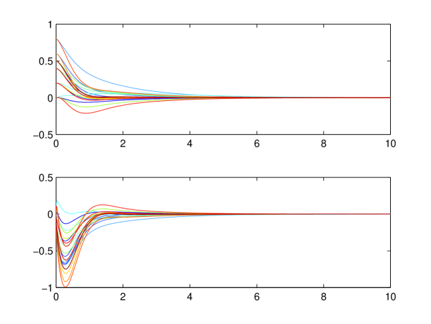
Figure 4: Relative angles (the top figure) and relative velocities of the pendulums with respect to the leader, obtained using the algorithm based on Theorems 1 and 5.

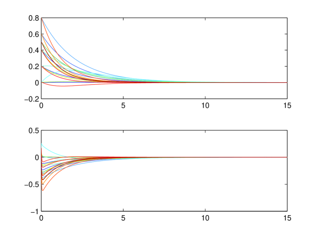
Figure 5: Relative angles (the top figure) and relative velocities of the pendulums with respect to the leader, obtained using the algorithm based on Theorems 2 and 6.

Figure 6: Relative angles (the top figure) and relative velocities of the pendulums with respect to the leader, obtained using the algorithm based on Theorems 3 and 7.

6 Conclusions

Two approaches to the leader-follower tracking control problem with guaranteed consensus tracking performance have been discussed in this paper. First, the problem was transformed into a decentralized control problem for a system, in which the interactions between subsystems satisfy integral quadratic constraints. This has allowed us to develop a procedure and sufficient conditions for the synthesis of a tracking consensus protocol for the original system. As this approach results in coupled LMIs which need to be solved simultaneously, we have also presented a result which does not involve coupled LMIs. Furthermore, an alternative method has been proposed which does not employ such a transformation, and instead uses overbounding of the performance cost. The latter method is shown to allow for an extension to encompass more general interconnected systems with nonidentical linear uncertain coupling operators. Also, this method can be extended to consider the interconnected systems with directed communication and interaction graphs (Cheng, Ugrinovskii & Wen, 2013).

These design techniques have been compared using an example. It is worth noting that the gaps between the predicted performance and computed performance among the three simulation results are considerably different. The method based on Theorem 1 exhibits the smallest gap out of the three results. The conservatism of Theorem 3 owes to the conservative upper bound on the original cost function in (37) and the particular form of the controller which made the inequality in (8.4) possible. These upper bounds have shown a noticeable effect in the example. The method based on Theorem 2 appears to be significantly more conservative than the methods based on Theorems 1 and 3. However, Theorem 2 enables the controller gain to be computed in a distributed manner, at the expense of degraded performance.

7 Funding

This work was supported by the Australian Research Council under the Discovery Projects funding scheme (projects DP0987369 and DP120102152).

8 Appendix

8.1 Proof of Lemma 1

Since the decentralized state feedback controller $\hat{u}_{i}=K\varepsilon_{i}$ solves the auxiliary decentralized guaranteed cost control problem for the collection of the systems (10), then there exist a constant $c>0$ such that

$$\sup_{\Xi,\Pi}\hat{\mathcal{J}}(\hat{u})<c.$$ (70)

Also we noted that every signal $\varphi$ which satisfies Assumption 1 gives rise to an admissible uncertainty for the large-scale system consisting of subsystems (10). This implies that for any $\varphi\in\Xi_{0}$, with $u=-\big{(}(\mathcal{L}^{c}+G)\otimes K\big{)}e$, we have

$$\mathcal{J}(u)=\hat{\mathcal{J}}(\hat{u})\leq\sup_{\Xi,\Pi}\hat{\mathcal{J}}(\hat{u})<c.$$ (71)

Therefore, one obtains $\sup\limits_{\Xi_{0}}\mathcal{J}(u)\leq\sup\limits_{\Xi,\Pi}\hat{\mathcal{J}}(\hat{u})<c$. It implies that the control protocol (3) with the same gain $K$ solves Problem 1.

8.2 Proof of Theorem 1

Using the Schur complement and substituting $F=KY$, the LMIs (25) can be transformed into the following Riccati inequality

$$Y^{-1}(A+\lambda_{i}B_{1}K)+(A+\lambda_{i}B_{1}K)^{\prime}Y^{-1}+\lambda_{i}^{2}K{{}^{\prime}}RK$$

$$+\Big{[}\frac{M_{i,i}^{2}}{{\pi}_{i}}+\frac{\sum\limits_{j\neq i}M_{i,j}^{2}}{{\theta}_{i}}\Big{]}Y^{-1}B_{2}B_{2}^{\prime}Y^{-1}+[Q_{i}+({\pi}_{i}+{\bar{\theta}}_{i})C^{\prime}C]<0,$$ (72)

where ${\bar{\theta}}_{i}=\sum\limits_{j\neq i}{\theta}_{i}$.

Consider the following Lyapunov function candidate for the interconnected system (10):

$$V(\varepsilon)=\sum_{i=1}^{N}\varepsilon_{i}^{\prime}Y^{-1}\varepsilon_{i}.$$ (73)

For the controller $\hat{u}_{i}=K\varepsilon_{i}$, using the Riccati inequality (8.2), we have

$$\frac{dV(\varepsilon)}{dt}< -\sum_{i=1}^{N}\varepsilon_{i}^{{}^{\prime}}\Big{(}\lambda_{i}^{2}K^{{}^{\prime}}RK+Q_{i}\Big{)}\varepsilon_{i}+\sum_{i=1}^{N}\Big{(}-\varepsilon_{i}^{{}^{\prime}}\frac{M_{i,i}^{2}}{{\pi}_{i}}Y^{-1}B_{2}B_{2}^{{}^{\prime}}Y^{-1}\varepsilon_{i}-2\varepsilon_{i}^{{}^{\prime}}Y^{-1}M_{i,i}B_{2}\xi_{i}$$

$$-{\pi}_{i}\|\xi_{i}\|^{2}+{\pi}_{i}\parallel\xi_{i}\parallel^{2}-{\pi}_{i}\parallel C\varepsilon_{i}\parallel^{2}-\frac{\sum\limits_{j\neq i}M_{i,j}^{2}}{{\theta}_{i}}\varepsilon_{i}^{{}^{\prime}}Y^{-1}B_{2}B_{2}^{{}^{\prime}}Y^{-1}\varepsilon_{i}$$

$$+2\varepsilon_{i}^{{}^{\prime}}Y^{-1}L_{i}\eta_{i}-{\theta}_{i}\parallel\eta_{i}\parallel^{2}+{\theta}_{i}\parallel\eta_{i}\parallel^{2}-{\bar{\theta}}_{i}\parallel C\varepsilon_{i}\parallel^{2}\Big{)}.$$ (74)

By completing the squares on the right hand side of (8.2) and using the identity

$$\sum\limits_{i=1}^{N}\sum\limits_{j\neq i}{\theta}_{i}\|C\varepsilon_{j}\|^{2}=\sum\limits_{i=1}^{N}{\bar{\theta}}_{i}\|C\varepsilon_{i}\|^{2},$$ (75)

we obtain

$$\int_{0}^{t_{l}}\frac{dV(\varepsilon)}{dt}dt <-\sum_{i=1}^{N}\int_{0}^{t_{l}}\varepsilon_{i}^{\prime}(\lambda_{i}^{2}K^{\prime}RK+Q_{i})\varepsilon_{i}dt-\sum_{i=1}^{N}\int_{0}^{t_{l}}\parallel\sqrt{{\pi}_{i}}\xi_{i}+\frac{1}{\sqrt{{\pi}_{i}}}M_{i,i}B_{2}^{{}^{\prime}}Y^{-1}\varepsilon_{i}\parallel^{2}dt$$

$$+\sum_{i=1}^{N}{\pi}_{i}\int_{0}^{t_{l}}(\parallel\xi_{i}\parallel^{2}-\parallel C\varepsilon_{i}\parallel^{2})dt-\sum_{i=1}^{N}\sum_{j\neq i}\int_{0}^{t_{l}}\parallel\sqrt{{\theta}_{i}}\xi_{j}+\frac{1}{\sqrt{{\theta}_{i}}}M_{i,j}B_{2}^{{}^{\prime}}Y^{-1}\varepsilon_{i}\parallel^{2}dt$$

$$+\sum_{i=1}^{N}{\theta}_{i}\int_{0}^{t_{l}}(\parallel\eta_{i}\parallel^{2}-\sum\limits_{j\neq i}\parallel C\varepsilon_{j}\parallel^{2})dt.$$

Here $t_{l}$ is an element of the sequence $\{t_{l}\}$ from Assumption 1. Finally, using the IQCs (13) and (14) and noting that $V(\varepsilon(t))\geq 0$, we obtain

$$\sum_{i=1}^{N}\int_{0}^{t_{l}}\varepsilon_{i}^{\prime}(\lambda_{i}^{2}K^{\prime}RK+Q_{i})\varepsilon_{i}dt<V(\varepsilon(0)).$$

The expression on the right hand side of the above inequality is independent of $t_{l}$. Letting $t_{l}\rightarrow\infty$ leads to $\hat{\mathcal{J}}(\hat{u})\leq V(\varepsilon(0))$. This conclusion holds for an arbitrary collection of inputs $\xi_{i}$, $\eta_{i}$ that satisfy (13), (14), respectively. Then $\sup\limits_{\Xi,\Pi}\hat{\mathcal{J}}(\hat{u})\leq e_{i}^{\prime}(0)Y^{-1}e_{i}(0)$. The claim of the theorem now follows from Lemma 1 and (71).

8.3 Proof of Theorem 2

Using Schur complement, the LMI (33) is equivalent to the following Riccati inequality

$$AY+YA^{\prime}-\frac{\underline{\lambda}^{2}}{\bar{\lambda}^{2}}B_{1}R^{-1}B_{1}^{\prime}+\Big{[}\frac{w^{2}}{{\pi}}+\frac{q^{2}}{{\theta}}\Big{]}B_{2}B_{2}^{\prime}+Y[\bar{\lambda}Q+({\pi}+\bar{\theta})C^{\prime}C]Y<0,$$ (76)

where $\bar{\theta}=(N-1){\theta}$.
Since $\underline{\lambda}\leq\lambda_{i}\leq\bar{\lambda}$, substituting $F=-\frac{\underline{\lambda}}{{\bar{\lambda}}^{2}}R^{-1}B_{1}^{\prime}$, $\pi_{i}=\pi$, $\theta_{i}=\theta$, $\bar{\theta}_{i}=(N-1)\theta=\sum\limits_{j\neq i}\theta_{i}$, $M_{i,i}^{2}\leq w^{2}$ and $\sum\limits_{j\neq i}M_{i,j}^{2}\leq q^{2}$, then we obtain

$$Y^{-1}(A+\lambda_{i}B_{1}K)+(A+\lambda_{i}B_{1}K)^{\prime}Y^{-1}+\lambda_{i}^{2}K{{}^{\prime}}RK$$

$$+\Big{[}\frac{M_{i,i}^{2}}{{\pi}_{i}}+\frac{\sum\limits_{j\neq i}M_{i,j}^{2}}{{\theta}_{i}}\Big{]}Y^{-1}B_{2}B_{2}^{\prime}Y^{-1}+[Q_{i}+({\pi}_{i}+{\bar{\theta}}_{i})C^{\prime}C]<0.$$ (77)

We obtain the Riccati inequality (8.2) which is equivalent to (25). The proof then readily follows from Theorem 1.

8.4 Proof of Theorem 3

The proof is similar to the proof of Theorem 1, therefore we only present the details which are different from that proof.

When $d_{i}\neq 0$ and $\Pi_{i}$ is as defined in (44), using Schur complement and substituting $K=-RB_{1}^{\prime}Y^{-1}$, the LMIs (50) are equivalent to the following Riccati inequality

$$Y^{-1}(A+\underline{\lambda}B_{1}K)+(A+\underline{\lambda}B_{1}K)^{\prime}Y^{-1}+\underline{\lambda}K^{\prime}RK$$

$$+(\frac{{f_{i}}^{2}}{\nu_{i}}+\sum\limits_{j\in S_{i}}\frac{1}{\mu_{ij}}+\frac{1}{\nu_{i0}}+\sum\limits_{k\colon d_{k}=1}\frac{1}{\mu_{0k}})Y^{-1}B_{2}B_{2}^{\prime}Y^{-1}+\bar{Q}+(\nu_{i}+\bar{\mu}_{i}+\nu_{i0}+N\mu_{0i})C^{\prime}C<0,$$ (78)

where $\bar{\mu}_{i}=\sum\limits_{j\colon i\in S_{j}}\mu_{ji}$.

When $d_{i}=0$ and $\Pi_{i}$ is defined in (49), a similar transformation results in the inequality

$$Y^{-1}(A+\underline{\lambda}B_{1}K)+(A+\underline{\lambda}B_{1}K)^{\prime}Y^{-1}+\underline{\lambda}K^{\prime}RK$$

$$+(\frac{{f_{i}}^{2}}{\nu_{i}}+\sum\limits_{j\in S_{i}}\frac{1}{\mu_{ij}}+\sum\limits_{k\colon d_{k}=1}\frac{1}{\mu_{0k}})Y^{-1}B_{2}B_{2}^{\prime}Y^{-1}+\bar{Q}+(\nu_{i}+\bar{\mu}_{i})C^{\prime}C<0.$$ (79)

Consider the quadratic Lyapunov function candidate $V(e)=\sum_{i=1}^{N}e_{i}^{\prime}Y^{-1}e_{i}$ for the interconnected system comprised of the subsystems (6). Since $K=-R^{-1}B_{1}^{\prime}Y^{-1}$, we have

$$\sum\limits_{i=1}^{N}2e_{i}^{\prime}Y^{-1}B_{1}K(\sum\limits_{j\in S^{c}_{i}}(e_{i}-e_{j})+g_{i}e_{i}) =-2e^{\prime}\big{(}(\mathcal{L}^{c}+G)\otimes(Y^{-1}B_{1}R^{-1}B_{1}^{\prime}Y^{-1})\big{)}e$$

$$\leq-2\sum\limits_{i=1}^{N}e_{i}^{\prime}\underline{\lambda}Y^{-1}B_{1}R^{-1}B_{1}^{\prime}Y^{-1}e_{i}.$$ (80)

It follows from (8.4) that

$$\frac{dV(e)}{dt} \leq\sum\limits_{i=1}^{N}2e_{i}^{\prime}Y^{-1}\Big{(}A+\underline{\lambda}B_{1}K\Big{)}e_{i}-2\sum\limits_{i=1}^{N}f_{i}e_{i}^{\prime}Y^{-1}B_{2}\varphi(t,e_{i}(.)|_{0}^{t})+2\sum\limits_{i=1}^{N}\sum\limits_{j\in S_{i}}e_{i}^{\prime}Y^{-1}B_{2}\varphi(t,e_{j}(.)|_{0}^{t})$$

$$-2\sum\limits_{i=1}^{N}\sum\limits_{k\colon d_{k}=1}e_{i}^{\prime}Y^{-1}B_{2}\varphi(t,e_{k}(.)|_{0}^{t})-2\sum\limits_{i=1}^{N}d_{i}e_{i}^{\prime}Y^{-1}B_{2}\varphi(t,e_{i}(.)|_{0}^{t}).$$ (81)

Then, using the Riccati inequalities (8.4) and (8.4), inequality (8.4), and the identities

$$\sum\limits_{i=1}^{N}\sum\limits_{j\in S_{i}}\mu_{ij}\|Ce_{j}\|^{2} =\sum\limits_{i=1}^{N}{\bar{\mu}_{i}}\|Ce_{i}\|^{2},$$

$$N\sum\limits_{i\colon d_{i}=1}\mu_{0i}e_{i}^{\prime}C^{\prime}Ce_{i} =N\sum\limits_{k\colon d_{k}=1}\mu_{0k}e_{k}^{\prime}C^{\prime}Ce_{k},$$

$$\sum\limits_{i=1}^{N}d_{i}e_{i}^{\prime}Y^{-1}B_{2}\varphi(t,e_{i}(.)|_{0}^{t}) =\sum\limits_{i\colon d_{i}=1}e_{i}^{\prime}Y^{-1}B_{2}\varphi(t,e_{i}(.)|_{0}^{t}),$$

in a manner similar to the proof of Theorem 1, we obtain the following bound

$$\sum\limits_{i=1}^{N}\int_{0}^{\infty}e_{i}^{\prime}\Big{(}\underline{\lambda}K^{\prime}RK+\bar{Q}\Big{)}e_{i}dt\leq V(e(0)).$$ (82)

Condition (51) now follows from (37) since $\bar{Q}=(\underline{\lambda}/\bar{\lambda})Q$.

It also implies that the control protocol (3) with $K=-R^{-1}B_{1}^{\prime}Y^{-1}$ solves Problem 1.

8.5 Proof of Theorem 5

Suppose the LMIs (25) and (60) have a feasible solution $Y,F,\pi_{i},\theta_{i}$ and $\gamma$, $i=1,\ldots,N$. Then it follows from (60) that

$$\sum_{i=1}^{N}e_{i}^{\prime}(0)Y^{-1}e_{i}(0)<\gamma.$$ (83)

Since the feasibility set of the LMIs (25), (60) is a subset of the feasibility set of the LMIs (25), then it follows from (83) that $\mathcal{J}_{\mbox{(\ref{LMI TH1})}}^{*}\leq\mathcal{J}_{\mbox{(\ref{LMI TH1}),(\ref{LMI minimize cost})}}^{*}$.

Conversely, for any sufficiently small $\rho>0$, there exist $Y,F,\theta_{i}$ and $\pi_{i}$, $i=1,\ldots,N$, verifying (25) such that

$$\mathcal{J}_{\mbox{(\ref{LMI TH1})}}^{*}+\rho>\sum_{i=1}^{N}e_{i}^{\prime}(0)Y^{-1}e_{i}(0).$$ (84)

Let $\gamma=\sigma+\sum_{i=1}^{N}e_{i}^{\prime}(0)Y^{-1}e_{i}(0)$, where $\sigma>0$ is an arbitrary constant. Then $\gamma,Y,F,\theta_{i}$ and $\pi_{i}$ satisfy conditions (25) and (60). Furthermore $\mathcal{J}_{\mbox{(\ref{LMI TH1}),(\ref{LMI minimize cost})}}^{*}\leq\gamma=\sigma+\sum_{i=1}^{N}e_{i}^{\prime}(0)Y^{-1}e_{i}(0)<\sigma+\rho+\mathcal{J}_{\mbox{(\ref{LMI TH1})}}^{*}$. Letting $\sigma$, $\rho\rightarrow 0$, we have $\mathcal{J}_{\mbox{(\ref{LMI TH1}),(\ref{LMI minimize cost})}}^{*}\leq\mathcal{J}_{\mbox{(\ref{LMI TH1})}}^{*}$. This completes the proof.

References

- Arenas et al. (2008) Arenas, A., Diaz-Guilera, A., Kurths, J., Moreno, Y., & Zhou, C. (2008). Synchronization in complex networks. Phys. Rep., 469(3), 93–153.
- Beard et al. (2002) Beard, R. W., McLain, T. W., Goodrich, M. A., & Anderson, E. P. (2002). Coordinated target assignment and intercept for unmanned air vehicles. IEEE Transactions on Robotics and Automation, 18(6), 911–922.
- Borrelli & Keviczky (2008) Borrelli, F., & Keviczky, T. (2008). Distributed LQR design for identical dynamically decoupled systems. IEEE Trans. Autom. Contr., 53, 1901–1912.
- Cheng & Ugrinovskii (2013) Cheng, Y., & Ugrinovskii, V. (2013). Guaranteed performance leader-follower control for multi-agent systems with linear IQC coupling. American Control Conference (pp. 2625–2630). Washington D.C., USA.
- Cheng, Ugrinovskii & Wen (2013) Cheng, Y., Ugrinovskii, V., & Wen, G (2013). Guaranteed cost tracking for uncertain coupled multi-agent systems using consensus over a directed graph. Australian Control Conference (pp. 375–378). Perth, Australia. Also, see arXiv:1309.0365.
- Cortes & Bullo (2003) Cortes, J., & Bullo, F. (2003). Coordination and geometric optimization via distributed dynamical systems. SIAM Journal on Control and Optimization, 44(5), 1543–1574.
- Fax & Murray (2004) Fax, A., & Murray, R. M., Information flow and cooperative control of vehicle formations. IEEE Trans. Autom. Contr., 49(9), 1465–1476.
- Franceschelli, Gasparri, Giua, & Seatzu (2013) Franceschelli, M., Gasparri, A., Giua, A., & Seatzu, C. (2013). Decentralized estimation of Laplacian eigenvalues in multi-agent systems. Automatica, 49, 1031–1036.
- Grip, Yang, Saberi, & Stoorvogel (2012) Grip, H. F., Yang T., Saberi, A., & Stoorvogel, A. A. (2012). Output synchronization for heterogeneous networks of non-introspective agents. Automatica, 48(10), 2444–2453.
- Hong, Hu, & Gao (2006) Hong, Y. G., Hu, J. P., & Gao, L. X. (2006). Tracking control for multi-agent consensus with an active leader and variable topology. Automatica, 42(7), 1177–1182.
- Jadbabaie, Lin, & Morse (2003) Jadbabaie, A., Lin, J., & Morse, S. A. (2003). Coordination of groups of mobile autonomous agents using nearest neighbor rules. IEEE Trans. Autom. Contr., 48(6), 988–1001.
- Li, Ugrinovskii, & Orsi (2007) Li, L., Ugrinovskii, V., & Orsi, R. (2007). Decentralized robust control of uncertain Markov jump parameter systems via output feedback. Automatica, 43, 1932–1944.
- Li, Duan, Chen, & Huang (2010) Li, Z. K., Duan, Z. S., Chen, G. R., & Huang, L. (2010). Consensus of multiagent systems and synchronization of complex networks: a unified viewpoint. IEEE Trans. Circuits and Systems, 57(1), 213–224.
- Megretski & Rantzer (1997) Megretski, A., & Rantzer, A. (1997). System analysis via integral quadratic constraints. IEEE Trans. Autom. Contr., 42(6), 819–830.
- Olfati-Saber (2006) Olfati-Saber, R. (2006). Flocking for multi-agent dynamic systems: theory and algorithms. IEEE Trans. Autom. Contr., 51(3), 401–420.
- Olfati-Saber, Fax, & Murray (2007) Olfati-Saber, R., Fax, J. A., & Murray, R. M. (2007). Consensus and cooperation in networked multi-agent systems. Proc. IEEE, 95(1), 215–233.
- Pecora & Carroll (1990) Pecora, L. M., & Carroll, T. L. (1990). Synchronization in chaotic systems. Phys. Rev. Lett., 64(8), 821–824.
- Persis, Sailer, & Wirth (2013) Persis, C. De, Sailer, R., & Wirth, F. (2013). Parsimonious event-triggered distributed control: A Zeno free approach. Automatica, 49, 2116–2124.
- Petersen, Ugrinovskii, & Savkin (2000) Petersen, I. R., Ugrinovskii, V., & Savkin, A. V. (2000). Robust control design using methods. London, U.K.: Springer-Verlag.
- Ren, Beard, & Atkins (2007) Ren, W., Beard, R. W., & Atkins, E. M. (2007). Information consensus in multivehicle cooperative control: Collective group behavior through local interaction. IEEE Control Syst. Mag., 27(2), 71–82.
- Ren & Atkins (2007) Ren, W., & Atkins, E. (2007). Distributed multi-vehicle coordinated control via local information exchange. Int. J. Robust Nonlinear Control, 17, 1002–1033.
- Trentelman, Takaba, & Monshizadeh (2013) Trentelman, H. L., Takaba, K., & Monshizadeh, N. (2013). Robust synchronization of uncertain linear multi-agent systems. IEEE Trans. Autom. Contr., 58(6), 1511–1523.
- Tuna (2008) Tuna, S. E. (2008). Synchronizing linear systems via partial-state coupling. Automatica, 44(8), 2179–2184.
- Tuna (2009) Tuna, S. E. (2009). Conditions for synchronizability in arrays of coupled linear systems. IEEE Trans. Autom. Contr., 54(10), 2416–2420.
- Ugrinovskii et al. (2000) Ugrinovskii, V., Petersen, I. R., Savkin, A. V., & Ugrinoskaya, E. Ya. (2000). Decentralized state-feedback stabilization and robust control of uncertain large-scale systems with integrally constrained interconnections. Syst. & Contr. Letters, 40, 107–119.
- Ugrinovskii & Pota (2005) Ugrinovskii, V., & Pota, H. R. (2005). Decentralized control of power systems via robust control of uncertain Markov jump parameter systems. International Journal of Control, 78(9), 662–677.
- Šiljak (1978) Šiljak, D. D. (1978). Large-scale dynamic systems: Stability and structure. New York, NY: North-Holland.
- Šiljak & Zecevic (2005) Šiljak, D. D., & Zecevic, A. I. (2005). Control of large-scale systems: Beyond decentralized feedback. Annual Reviews in Control, 29, 169 -179.
- Wieland, Sepulchre, & Allgöwer (2011) Wieland, P., Sepulchre, R., & Allgöwer, F. (2011). An internal model principle is necessary and sufficient for linear output synchronization. Automatica, 47(5), 1068–1074.
- Willems (1971) Willems, J. C. (1971). The analysis of feedback systems. Cambridge, MA: MIT Press.
- Zhang, Lewis, & Das (2011) Zhang, H. W., Lewis, F. L., & Das, A. (2011). Optimal design for synchronization of cooperative systems: State feedback, observer and output feedback. IEEE Trans. Autom. Contr., 56(8), 1948–1952.
- Zhao, Duan, Wen & Chen (2012) Zhao, Y., Duan, Z., Wen G., & Chen G. (2012). Distributed H∞ consensus of multi-agent systems: a performance region-based approach. International Journal of Control, 85(3), 332–341.
- Zhao, Li, & Duan (2013) Zhao, Y., Li Z., & Duan, Z. (2013). Distributed consensus tracking of multi-agent systems with nonlinear dynamics under a reference leader. International Journal of Control, 86(10), 1859–1869.