A fast Mixed Model B-splines algorithm

Abstract

A fast algorithm for B-splines in mixed models is presented. B-splines have local support and are computational attractive, because the corresponding matrices are sparse. A key element of the new algorithm is that the local character of B-splines is preserved, while in other existing methods this local character is lost. The computation time for the fast algorithm is linear in the number of B-splines, while computation time scales cubically for existing transformations.

1 Introduction

Penalized regression using B-splines can be computationally efficient, because of the local character of B-splines. The corresponding linear equations are sparse and can be solved quickly. However, the main problem is to find the optimal value for the penalty parameter. A good way to approach this problem is to use mixed models and restricted maximum likelihood citep(REML; Patterson & Thompson, 1971). Several methods have been proposed to transform the original penalized B-spline model to a mixed model citep(Currie & Durbán, 2002; Lee & Durbán, 2011). A problem with existing transformations to mixed models is that the local character of the B-splines is lost, which reduces the computational efficiency. For relatively small datasets this is not a major issue. However, for long time series, for example with measurements every five minutes for several months, the computational efficiency becomes quite important.

In this paper I present a new transformation to a mixed model. This model is closely related to the transformation proposed by citeCurrie & Durbán (2002). However, the computation time in the transformation of citeCurrie & Durbán (2002) increases cubically in the number of B-splines, while for the new transformation the computation time increases linearly in time, using sparse matrix algebra citep(Furrer & Sain, 2010). One of the key elements of the proposed algorithm is that the transformation preserves the local character of B-splines, and all the equations can be solved quickly.

The paper is organized as follows. In Section 2 relevant information about B-splines is given. In Section (3) first the P-spline model citep(Eilers & Marx, 1996) is described and the transformation to mixed models by citeCurrie & Durbán (2002) is stated. The new transformation is presented, and details for a sparse mixed model formulation are given. In Section 4 the R-code is briefly described and a comparison is made between the computation time of the new method and the transformation by citeCurrie & Durbán (2002).

2 B-splines

In this preliminary section, a few relevant details about B-splines are given. For a detailed overview of B-splines, see for example citeDe Boor (1978) and citeHastie et al. (2009). B-splines have local support. This property is important and can speedup calculations considerably. To illustrate the idea of the local support, see Figure 1, with quadratic (i.e. degree $q=2$) B-splines. Throughout the paper we will assume equal distance between the splines, denoted by $h$. In the example presented in Figure 1 the distance is unity, $h=1$. The number of B-splines will be denoted by $m$. The first quadratic B-spline, $B_{1,2}(x)$ is zero outside the interval $[-2,1]$. The last one, $B_{12,2}(x)$, is zero outside the interval $[9,12]$. So, for this example, there are $m=12$ quadratic B-splines which define the B-spline basis for the domain $[x_{\text{min}},x_{\text{max}}]=[0,10]$ of interest.

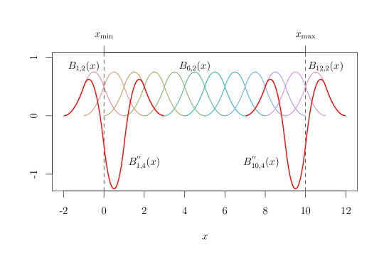
Figure 1: Quadratic B-spline basis for the interval $[x_{\text{min}},x_{\text{max}}]=[0,10]$, formed by $B_{1,2}(x)$, $B_{2,2}(x)$, … , $B_{12,2}(x)$. The distance between the splines is unity. The red curves are second-order derivatives of quartic B-splines; for clarity only the first and last one are shown. The second-order derivatives of quartic B-splines can be constructed from quadratic B-splines, see equation (1).

The second derivative of B-splines is given by citep(De Boor, 1978):

$$h^{2}B^{{}^{\prime\prime}}_{j,q}(x)=B_{j,q-2}(x)-2B_{j+1,q-2}(x)+B_{j+2,q-2}(x)\;.$$ (1)

The second derivative is illustrated in Figure 1. The red curves are second-order derivatives of quartic (fourth-degree) B-splines. As can be seen from equation (1) it can represented as a linear combination of three quadratic B-splines.

3 P-splines and Mixed Models

In this section we will give a brief description of P-splines citep(Eilers & Marx, 1996). Let $n$ be the number of observations. Suppose the variable $\mathbf{y}=(y_{1},\ldots,y_{n})^{\prime}$ depends smoothly on the variable $\mathbf{x}=(x_{1},\ldots,x_{n})^{\prime}$. Let $\mathbf{B}=(B_{1,2}(\mathbf{x}),\ldots,B_{m,2}(\mathbf{x}))$ be a $n\times m$ matrix, and $\mathbf{a}=(a_{1},a_{2},\ldots,a_{m})^{\prime}$ be a vector of regression coefficients. Then the following objective function to be minimized can be defined:

$$S(\mathbf{a})=(\mathbf{y}-\mathbf{B}\mathbf{a})^{\prime}(\mathbf{y}-\mathbf{B}\mathbf{a})+\lambda\;\mathbf{a}^{\prime}\mathbf{D}^{\prime}\mathbf{D}\mathbf{a}\;,$$ (2)

where $\lambda>0$ is a penalty or regularization parameter, and $\mathbf{D}$ is an $(m-2)\times m$ second-order difference matrix citep(see e.g. Eilers & Marx, 1996).

citeCurrie & Durbán (2002) showed that equation (2) can be reformulated as a mixed model:

$$\mathbf{y}=\mathbf{Xb}+\mathbf{Zu}+\mathbf{e}\;,\quad\mathbf{u}\backsim N(\mathbf{0},\frac{1}{\lambda}\mathbf{Q}^{-1}\sigma^{2})\;,\quad\mathbf{e}\backsim N(\mathbf{0},\mathbf{I}\sigma^{2})\;,$$ (3)

where $\mathbf{X}$ and $\mathbf{Z}$ are design matrices, $\mathbf{Q}$ is a precision matrix, $\mathbf{b}=(b_{0},b_{1})^{\prime}$ are the fixed effects, $\mathbf{u}=(u_{1},u_{2},\ldots,u_{m-2})^{\prime}$ the random effects, $\mathbf{e}$ is the residual error, and $\sigma^{2}$ is the residual variance.

citeCurrie & Durbán (2002) used the following transformation:

$$\mathbf{a}=\mathbf{G}\mathbf{b}+\mathbf{D}^{\prime}(\mathbf{D}\mathbf{D}^{\prime})^{-1}\mathbf{u}\;,$$ (4)

where $\mathbf{G}$ is an $m\times 2$ matrix with columns $\mathbf{g}_{0}=(1,1,\ldots,1)^{\prime}$ and $\mathbf{g}_{1}=(1,2,\ldots,m)^{\prime}$. This transformation gives the following expressions for the design matrices and the precision matrix:

$$\mathbf{X}=\mathbf{B}\mathbf{G}\;,\quad\mathbf{Z}=\mathbf{B}\mathbf{D}^{\prime}(\mathbf{D}\mathbf{D}^{\prime})^{-1}\;,\quad\mathbf{Q}=\mathbf{I}\;.$$ (5)

The mixed model equations citep(Henderson, 1963) corresponding to equation (3) are given by:

$$\begin{pmatrix}\mathbf{X^{\prime}X}&\mathbf{X^{\prime}Z}\\ \mathbf{Z^{\prime}X}&\mathbf{Z^{\prime}Z}+\lambda\mathbf{Q}\end{pmatrix}\begin{pmatrix}\widehat{\mathbf{b}}\\ \widehat{\mathbf{u}}\end{pmatrix}=\begin{pmatrix}\mathbf{X^{\prime}y}\\ \mathbf{Z^{\prime}y}\end{pmatrix}\;.$$ (6)

The coefficient matrix $\mathbf{C}_{\lambda}$ in equation (6) is given by:

$$\mathbf{C}_{\lambda}=\begin{pmatrix}\mathbf{X^{\prime}X}&\mathbf{X^{\prime}Z}\\ \mathbf{Z^{\prime}X}&\mathbf{Z^{\prime}Z}+\lambda\mathbf{Q}\end{pmatrix}\;.$$ (7)

This coefficient matrix is dense, since the local character of the B-splines has been destroyed by equation (5). This implies that the computation complexity for solving equation (6) is $\mathcal{O}(m^{3})$.

The following transformation preserves the local character of the B-splines:

$$\mathbf{a}=\mathbf{G}\mathbf{b}+\mathbf{D}^{\prime}\mathbf{u}\;.$$ (8)

Figure 1 illustrates the underlying idea of this transformation. The quadratic B-splines basis consists of $m=12$ B-splines. This quadratic B-spline basis is transformed to a second-order derivative quartic B-splines basis of $m-2=10$ B-splines, plus a parameter for intercept $b_{0}$ and linear trend $b_{1}$. The second-order derivative quartic B-splines can be constructed from quadratic B-splines by second-order differencing. Using the new transformation the design and precision matrices are given by:

$$\mathbf{X}=\mathbf{B}\mathbf{G}\;,\quad\mathbf{Z}=\mathbf{B}\mathbf{D}^{\prime}\;,\quad\mathbf{Q}=\mathbf{D}\mathbf{D}^{\prime}\mathbf{D}\mathbf{D}^{\prime}\;.$$ (9)

Let us refer to equations (3) and (9) as a Mixed Model of B-splines (MMB), since it uses the B-splines directly as building blocks for the mixed model. The matrix $\mathbf{Z}^{\prime}\mathbf{Z}+\lambda\mathbf{Q}$ has bandwidth $4$. This implies that $\mathbf{C}_{\lambda}$ is sparse and computation complexity has been reduced to $\mathcal{O}(m)$. An efficient way to calculate the REML profile log likelihood citep(Gilmour et al., 1995; Crainiceanu & Ruppert, 2004; Searle et al., 2009) is given by the following four steps :

1. Sparse Cholesky factorization citep(Furrer & Sain, 2010): $\mathbf{C}_{\lambda}=\mathbf{U}_{\lambda}\mathbf{U}^{{}^{\prime}}_{\lambda}$, where $\mathbf{U}_{\lambda}$ is an upper-triagonal matrix.

2. Forward-solve and back-solve citep(Furrer & Sain, 2010), with $\mathbf{w}$ a vector of length $m$:

   $$\mathbf{U}_{\lambda}\mathbf{w}=\begin{pmatrix}\mathbf{X^{\prime}y}\\ \mathbf{Z^{\prime}y}\end{pmatrix}\;,\quad\mathbf{U}^{{}^{\prime}}_{\lambda}\begin{pmatrix}\widehat{\mathbf{b}}\\ \widehat{\mathbf{u}}\end{pmatrix}=\mathbf{w}\;.$$ (10)

3. Calculate $\hat{\sigma}^{2}$ citep(Johnson & Thompson, 1995), $p$ is the dimension of the fixed effects:

   $$\hat{\sigma}^{2}=\frac{\mathbf{y}^{\prime}\mathbf{y}-\widehat{\mathbf{b}}^{\prime}\mathbf{X}^{\prime}\mathbf{y}-\widehat{\mathbf{u}}^{\prime}\mathbf{Z}^{\prime}\mathbf{y}}{n-p}\;.$$ (11)

4. REML log profile likelihood citep(Gilmour et al., 1995; Crainiceanu & Ruppert, 2004; Searle et al., 2009):

   $$L(\lambda)=-\frac{1}{2}\left(2\log|\mathbf{U}_{\lambda}|-(m-p)\log\lambda+(n-p)\log\hat{\sigma}^{2}+C\right)\;,$$ (12)

   where $C$ is a constant: $C=n-p-\log|\mathbf{Q}|$.

A one-dimensional optimization algorithm can be used to find the maximum for $L(\lambda)$. The computation time is linear in $m$.

4 R-package MMBsplines

An R-package, MMBsplines, is available at GitHub:

https://github.com/martinboer/MMBsplines.git.

The sparse matrix calculations are done with the spam package citeFurrer & Sain (2010). The B-splines are constructed with splineDesign() of the splines library.

The following example code sets some parameter values and runs the simulations:

    nobs = 1000; xmin = 0; xmax = 10
    set.seed(949030)
    sim.fun = function(x) { return(3.0 + 0.1*x + sin(2*pi*x))}
    x = runif(nobs, min = xmin, max = xmax)
    y = sim.fun(x) + 0.5*rnorm(nobs)

A fit to the data on a small grid can be obtained as follows, using $m=100$ quadratic B-splines:

    obj = MMBsplines(x, y, xmin, xmax, nseg = 100)
    x0 = seq(xmin, xmax, by=0.01)
    yhat = predict(obj, x0)
    ylin = predict(obj, x0, linear = TRUE)
    ysim = sim.fun(x0)

Figure 2 shows the result, with $\lambda_{\text{max}}=1.33$.

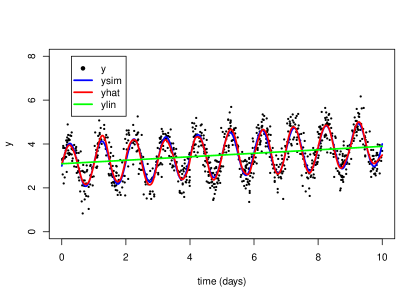
Figure 2: Fit of the simulated data using MMBsplines, with $\lambda_{\text{max}}=1.33$. The blue line is the true simulated line, the red line is the fitted value. The green line is the linear trend.

The Currie and Durban transformation can be run by setting the sparse argument to FALSE:

    obj = MMBsplines(x, y, xmin, xmax, nseg = 100, sparse = FALSE)

For $m=100$, as in Figure 2, the differences in computation time are small. If we increase the length of the simulated time series, with a fixed stepsize $h=0.1$, the advantage of the MMB-splines method becomes clear, see Figure 3. As expected the Currie and Durban transformation computation time increases cubical in the number of B-splines, computatation time for MMB-splines is linear in $m$.

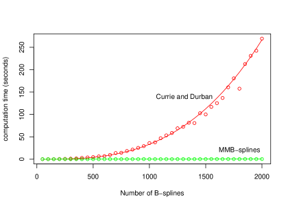
Figure 3: Comparison of computation times. The computation time for the Currie and Durban transformation is cubical in the number of B-splines. The computation time for MMB-splines is linear in the number of B-splines.

5 Conclusion

The MMB-splines method presented in this paper seems to be an attractive way to use B-splines in mixed models. The method was only presented for quadratic splines, but also cubical or higher-degree B-splines could have been used. Other generalizations are also possible, for example extension to multiple penalties citep(Currie & Durbán, 2002) or multiple dimensions citep(Rodríguez-Álvarez et al., 2014).

References

- Crainiceanu & Ruppert (2004) Crainiceanu, C., & Ruppert, D. (2004). Likelihood ratio tests in linear mixed models with one variance component. Journal of the Royal Statistical: Series B, 66, 165-185.
- Currie & Durbán (2002) Currie, I., & Durbán, M. (2002). Flexible smoothing with P-splines: a unified approach. Statistical Modelling, 4, 333-349.
- De Boor (1978) De Boor, C. (1978). A practical guide to splines. Mathematics of Computation.
- Eilers & Marx (1996) Eilers, P., & Marx, B. (1996). Flexible smoothing with B-splines and penalties. Statistical science, 11, 89-121.
- Furrer & Sain (2010) Furrer, R., & Sain, S. (2010). spam: A sparse matrix R package with emphasis on MCMC methods for Gaussian Markov random fields. Journal of Statistical Software, 36, 1-25.
- Gilmour et al. (1995) Gilmour, A., Thompson, R., & Cullis, B. (1995). Average information REML: an efficient algorithm for variance parameter estimation in linear mixed models. Biometrics, 51, 1440-1450.
- Hastie et al. (2009) Hastie, T., Tibshirani, R., & Friedman, J. (2009). The elements of statistical learning. Springer.
- Henderson (1963) Henderson, C. (1963). Selection index and expected genetic advance. Statistical genetics and plant breeding, NAS-NRC 1982.
- Johnson & Thompson (1995) Johnson, D., & Thompson, R. (1995). Restricted maximum likelihood estimation of variance components for univariate animal models using sparse matrix techniques and average information. Journal of dairy science, 78, 449-456.
- Lee & Durbán (2011) Lee, D., & Durbán, M. (2011). P-spline ANOVA-type interaction models for spatio-temporal smoothing. Statistical Modelling, 11, 49-69.
- Patterson & Thompson (1971) Patterson, H., & Thompson, R. (1971). Recovery of inter-block information when block sizes are unequal. Biometrika, 58, 545-554.
- Rodríguez-Álvarez et al. (2014) Rodríguez-Álvarez, M., Lee, D., Kneib, T., Durbán, M., & Eilers, P. (2014). Fast smoothing parameter separation in multidimensional generalized P-splines: the SAP algorithm. Statistics and Computing, 1-17.
- Searle et al. (2009) Searle, S., Casella, G., & McCulloch, C. (2009). Variance components. John Wiley and Sons.