A fictitious domain finite element method for simulations of fluid-structure interactions: The Navier-Stokes equations coupled with a moving solid

Abstract

The paper extends a stabilized fictitious domain finite element method initially developed for the Stokes problem to the incompressible Navier-Stokes equations coupled with a moving solid. This method presents the advantage to predict an optimal approximation of the normal stress tensor at the interface. The dynamics of the solid is governed by the Newton’s laws and the interface between the fluid and the structure is materialized by a level-set which cuts the elements of the mesh. An algorithm is proposed in order to treat the time evolution of the geometry and numerical results are presented on a classical benchmark of the motion of a disk falling in a channel.

1 Introduction

Fluid-structure interactions problems remain a challenge both for a comprehensive study of such problems as for the development of robust numerical methods (see a review in [1]). One class of numerical methods is based on meshes that are conformed to the interface where the physical boundary conditions are imposed [2, 3, 4]. As the geometry of the fluid domain changes through the time, re-meshing is needed, which is excessively time-consuming, in particular for complex systems. An other class of numerical methods is based on non-conforming mesh with a fictitious domain approach where the mesh is cut by the boundary. Most of the non-conforming mesh methods are based on the immersed boundary methods where force-equivalent terms are added to the fluid equations in order to represent the fluid structure interaction [5, 6]. Many related numerical methods have been developed, in particular the popular distributed Lagrange multiplier method, introduced for rigid bodies moving in an incompressible flow [7]. In this method, the fluid domain is extended in order to cover the rigid domain where the fluid velocity is required to be equal to the rigid body velocity.
More recently, eXtended Finite Element Method introduced by Moës, Dolbow and Belytschko in [8] (see a review of such methods in [9]) has been adapted to fluid structure interactions problems in [10, 11, 12, 13]. The idea is similar to the fictitious domain / Lagrange multiplier method aforementioned, but the fluid velocity is no longer extended inside the structure domain, and its value given by the structure velocity is enforced by a Lagrange multiplier only on the fluid-structure interface. One thus gets rid of unnecessary fluid unknowns. Besides, one easily recovers the normal trace of the Cauchy stress tensor on the interface. We note that this method has been originally developed for problems in structural mechanics mostly in the context of cracked domains, see for example [14, 15, 16, 17, 18]. The specificity of the method is that it combines a level-set representation of the geometry of the crack with an enrichment of a finite element space by singular and discontinuous functions.
In the context of fluid-structure interactions, the difficulty related to the applications of such techniques lies in the choice of the Lagrange multiplier space used in order to take into account the interface, which is not trivial because of the fact that the interface cuts the mesh (see [19] for instance). In particular, the natural mesh given by the points of intersection of the interface with the global mesh cannot be used directly. An algorithm to construct a multiplier space satisfying the inf-sup condition is developed in [19], but its implementation can be difficult in practice. The method proposed in the present paper tackles this difficulty by using a stabilization technique proposed in [14]. This method was adapted to contact problems in elastostatics in [20] and more recently to the Stokes problem in [21]. An important feature of this method (based on the eXtended Finite Element Method approach, similarly to [12, 13]) is that the Lagrange multiplier is identified with the normal trace of the Cauchy stress tensor $\sigma(\boldsymbol{\mathrm{u}},p)\boldsymbol{\mathrm{n}}$ at the interface. Moreover, it is possible to obtain a good numerical approximation of $\sigma(\boldsymbol{\mathrm{u}},p)\boldsymbol{\mathrm{n}}$ (the proof is given in [21] for the Stokes problem). This property is crucial in fluid-structure interactions since this quantity gives the force exerted by the viscous fluid on the structure. In the present paper, we propose to extend this method to the Navier-Stokes equations coupled with a moving solid. Note that alternative methods based on the Nitsche’s work [22] (such as [23, 24] in the context of the Poisson problem and [25] in the context of the Stokes problems) do not introduce the Lagrange multiplier and thus do not necessarily provide a good numerical approximation of this force. Our method based on boundary forces is particular interesting for control flow around a structure. The control function can be localized on the boundary of the structure where we impose its local deformation. In order to perform direct numerical simulations of such a control, efficient tools based on accurate computations on the interface must be developed. The present approach is one brick in this research topic where recent development towards stabilized Navier-Stokes equations are proposed (like in [26]).

The outline of the paper is as follows. The continuous fluid-structure interactions problem is given in Section 2 and the weak formulation with the introduction of a Lagrange multiplier for imposing the boundary condition at the interface is given in Section 2.2. Next, in Section 3 the fictitious domain method is recalled with the introduction of the finite element method (Section 3.1) with a time discretization (Section 3.2). Section 4 is devoted to numerical tests and validation on a benchmark corresponding to the falling of a disk in a channel. The efficiency of the method is presented before conclusion.

2 The model

2.1 Fluid-structure interactions

We consider a moving solid which occupies a time-depending domain denoted by $\mathcal{S}(t)$. The remaining domain $\mathcal{F}(t)=\mathcal{O}\setminus\overline{\mathcal{S}(t)}$ corresponds to the fluid flow.

Figure 1: Decomposition of the solid movement.

The displacement of a rigid solid can be given by the knowledge of ${\bf h}(t)$, namely the position of its gravity center, and $\mathbf{R}(t)$ its rotation given by $\displaystyle\left(\begin{array}[]{cc}c&-s\\ s&c\\ \end{array}\right)$ for $\displaystyle c=\cos(\theta(t))$, $s=\sin(\theta(t))$, where $\theta(t)$ is the rotation angle of the solid (see Figure 1). Then at time $t$ the domain occupied by the structure is given by

$$\displaystyle\mathcal{S}(t) = {\bf h}(t)+\mathbf{R}(t)\mathcal{S}(0).$$

Remark: This formulation can be extended in order to consider general deformations of the structure. Then we would have to define a mapping $X^{*}(\cdot,t)$ which corresponds to the deformation of the solid in its own frame of reference. Then, $\mathcal{S}(t)=X_{S}(\mathcal{S}(0),t)$ where $X_{S}(\mathrm{y},t)={\bf h}(t)+\mathbf{R}(t)X^{*}(\mathrm{y},t)$, for $\mathrm{y}\in\mathcal{S}(0)$.

The velocity of the incompressible viscous fluid of density $\rho_{f}$ is denoted by ${\bf u}$, the pressure by $p$ and $\nu$ is the dynamic viscosity. We denote by $\boldsymbol{\mathrm{n}}$ the outward unit normal vector to $\partial\mathcal{F}$ (the boundary of $\mathcal{F}$), and the normal trace on the interface $\Gamma=\partial\mathcal{S}(t)$ of the Cauchy stress tensor is given by

$$\sigma(\boldsymbol{\mathrm{u}},p)\boldsymbol{\mathrm{n}}=2\nu D(\boldsymbol{\mathrm{u}}){\bf n}-p\boldsymbol{\mathrm{n}}, \text{ with }D(\boldsymbol{\mathrm{u}})=\frac{1}{2}\left(\nabla\boldsymbol{\mathrm{u}}+\nabla\boldsymbol{\mathrm{u}}^{T}\right).$$

When gravity forces are considered (we denote by ${\bf g}$ the gravity field), the fluid flow is modeled by the incompressible Navier-Stokes equations

$$\left\{\begin{array}[]{llr}\displaystyle\rho_{f}\left(\frac{\partial{\bf u}}{\partial t}+({\bf u}.\nabla){\bf u}\right)-\nu\Delta{\bf u}+\nabla p=\rho_{f}{\bf g},&\mathrm{x}\in\mathcal{F}(t),&t\in(0,T),\\ \displaystyle\mbox{div}({\bf u})=0,&\mathrm{x}\in\mathcal{F}(t),&t\in(0,T),\\ \displaystyle{\bf u}=0,&\mathrm{x}\in\partial\mathcal{O},&t\in(0,T),\\ \end{array}\right.$$ (1)

and the Newton’s laws are considered for the dynamics of the solid

$$\left\{\begin{array}[]{l}\displaystyle m_{s}{\bf h}^{\prime\prime}(t)=-\int_{\partial\mathcal{S}(t)}{\sigma({\bf u},p){\bf n}}d\Gamma-m_{s}{\bf g},\\ \displaystyle I\theta^{\prime\prime}(t)=-\int_{\partial\mathcal{S}(t)}({\bf x}-{\bf h}(t))^{\bot}\cdot{\sigma({\boldsymbol{\mathrm{u}}},p){\bf n}}d\Gamma,\end{array}\right.$$ (2)

where $m_{s}$ is the mass of the solid, and $I$ is its moment of inertia.
At the interface $\partial\mathcal{S}(t)$, for the coupling between fluid and structure, we impose the continuity of the velocity

$${\bf u}({\bf x},t)={\bf h}^{\prime}(t)+\theta^{\prime}(t)({\bf x}-{\bf h}(t))^{\bot}={\bf u_{\Gamma}},\ \ \ {\bf x}\in\partial\mathcal{S}(t),\ \ \ t\in(0,T).$$ (3)

The coupled system (1)–(3) has for unknowns ${\bf u}$, $p$, ${\bf h}(t)$ and the angular velocity $\omega(t)=\theta^{\prime}(t)$ (a scalar function in 2D).

2.2 Weak formulation of the problem with stabilization terms

We consider the coupled system (1)-(3) and we assume that the boundary condition imposed at the interface $\Gamma=\partial\mathcal{S}(t)$ is sufficiently regular to make sense, and we introduce the following functional spaces (based on the classical Sobolev spaces $\mathrm{L}^{2}(\mathcal{F})$, $\mathbf{H}^{1}(\mathcal{F})$, $\mathbf{H}^{1/2}(\Gamma)$ and $\mathbf{H}^{-1/2}(\Gamma)$, see [27] for instance)

$$\begin{array}[]{lcl}\mathbf{V}&=&\left\{\boldsymbol{\mathrm{v}}\in\mathbf{H}^{1}(\mathcal{F})\mid\boldsymbol{\mathrm{v}}=0\text{ on }\partial\mathcal{O}\right\},\\ Q&=&\mathrm{L}^{2}_{0}(\mathcal{F})=\left\{p\in\mathrm{L}^{2}(\mathcal{F})\mid\displaystyle\int_{\mathcal{F}}p\ \mathrm{d}\mathcal{F}=0\right\},\\ \mathbf{W}&=&\mathbf{H}^{-1/2}(\Gamma)=\left(\mathbf{H}^{1/2}(\Gamma)\right)^{\prime}.\\ \end{array}$$

Due to the fact that we only consider boundary conditions of Dirichlet type, we impose to the pressure $p$ to have null average (this condition is taken into account in $Q$). That variational formulation can be done in three steps:

• Classical formulation of the Navier-Stokes and structure equations (in the formulation $\gamma$ and $\boldsymbol{\mathrm{\lambda}}$ are equal to $0$);

• Introduction of Lagrange multiplier $\boldsymbol{\mathrm{\lambda}}$ in order to take into account the Dirichlet condition at the interface $\Gamma$ (in the formulation only $\gamma$ is equal to $0$);

• Introduction of stabilization terms with a parameter $\gamma$.

This new unknown $\boldsymbol{\mathrm{\lambda}}$ plays a critical role due to the fact that it is equal to the normal trace of the Cauchy stress tensor $\sigma(\boldsymbol{\mathrm{u}},p)\boldsymbol{\mathrm{n}}$ (this equality is described in [28]). The stabilization terms are associated with the constant parameter $\gamma$ (chosen sufficiently small). The variational problem that we consider is the following:

Find $$({\bf u},p,{\bf\lambda},{\bf h}^{\prime},{\bf h},\theta^{\prime},\theta)\in\mathbf{V}\times Q\times\mathbf{W}\times\mathbb{R}^{2}\times\mathbb{R}^{2}\times\mathbb{R}\times\mathbb{R}$$ such that

$$\left\{\begin{array}[]{ll}\displaystyle\int_{\mathcal{F}}\rho_{f}\frac{\partial{\bf u}}{\partial t}\cdot{\bf v}\mathrm{d}\mathcal{F}+\mathcal{A}(({\bf u},p,{\boldsymbol{\mathrm{\lambda}}});{\bf v})+\int_{\mathcal{F}}\rho_{f}[({\bf u}\cdot\nabla){\bf u}]\cdot{\bf v}\mathrm{d}\mathcal{F}=\int_{\mathcal{F}}\rho_{f}{\bf g}\cdot{\bf v}\mathrm{d}\mathcal{F},&\forall{\bf v}\in\mathbf{V},\\ \mathcal{B}(({\bf u},p,\boldsymbol{\lambda});q)=0,&\forall q\in Q,\\ \mathcal{C}(({\bf u},p,\boldsymbol{\lambda});{\boldsymbol{\mathrm{\mu}}})=\mathcal{G}({\boldsymbol{\mathrm{\mu}}}),&\forall{\bf\boldsymbol{\mathrm{\mu}}}\in\mathbf{W},\\ \displaystyle m_{s}{\bf h}^{\prime\prime}(t)=-\int_{\partial\mathcal{S}(t)}{\boldsymbol{\mathrm{\lambda}}}d\Gamma-m_{s}{\bf g},&\\ \displaystyle I\theta^{\prime\prime}(t)=-\int_{\partial\mathcal{S}(t)}({\bf x}-{\bf h}(t))^{\bot}\cdot\boldsymbol{\lambda}d\Gamma,&\end{array}\right.$$

where

$$\mathcal{A}(({\bf u},p,\boldsymbol{\lambda});{\bf v}) = 2\nu\int_{\mathcal{F}}D({\bf u}):D({\bf v})\mathrm{d}\mathcal{F}-\int_{\mathcal{F}}p\mathrm{div}\ {\bf v}\mathrm{d}\mathcal{F}-\int_{\Gamma}\boldsymbol{\lambda}\cdot{\bf v}\mathrm{d}\Gamma$$

$$-4\nu^{2}\gamma\int_{\Gamma}\left(D({\bf u})\boldsymbol{\mathrm{n}}\right)\cdot\left(D({\bf v})\boldsymbol{\mathrm{n}}\right)\mathrm{d}\Gamma+2\nu\gamma\int_{\Gamma}p\left(D({\bf v})\boldsymbol{\mathrm{n}}\cdot\boldsymbol{\mathrm{n}}\right)\mathrm{d}\Gamma+2\nu\gamma\int_{\Gamma}\boldsymbol{\lambda}\cdot\left(D({\bf v})\boldsymbol{\mathrm{n}}\right)\mathrm{d}\Gamma,$$

$$\mathcal{B}(({\bf u},p,\boldsymbol{\lambda});q) = -\int_{\mathcal{F}}q\mathrm{div}\ {\bf u}\mathrm{d}\mathcal{F}+2\nu\gamma\int_{\Gamma}q\left(D({\bf u})\boldsymbol{\mathrm{n}}\cdot\boldsymbol{\mathrm{n}}\right)\mathrm{d}\Gamma-\gamma\int_{\Gamma}pq\mathrm{d}\Gamma-\gamma\int_{\Gamma}q\boldsymbol{\lambda}\cdot\boldsymbol{\mathrm{n}}\mathrm{d}\Gamma,$$

$$\mathcal{C}(({\bf u},p,\boldsymbol{\lambda});\boldsymbol{\mu}) = -\int_{\Gamma}\boldsymbol{\mu}\cdot{\bf u}\mathrm{d}\Gamma+2\nu\gamma\int_{\Gamma}\boldsymbol{\mu}\cdot(D({\bf u})\boldsymbol{\mathrm{n}})\mathrm{d}\Gamma-\gamma\int_{\Gamma}p(\boldsymbol{\mu}\cdot\boldsymbol{\mathrm{n}})\mathrm{d}\Gamma-\gamma\int_{\Gamma}\boldsymbol{\lambda}\cdot\boldsymbol{\mu}\mathrm{d}\Gamma,$$

$$\mathcal{G}(\boldsymbol{\mu}) = -\int_{\Gamma}\boldsymbol{\mu}\cdot{\bf u_{\Gamma}}\mathrm{d}\Gamma=-\int_{\Gamma}\boldsymbol{\mu}\cdot({\bf h}^{\prime}(t)+\theta^{\prime}(t)({\bf x}-{\bf h}(t))^{\bot})\mathrm{d}\Gamma.$$

Remark: The formulation can be justified by the introduction of an extended Lagrangian - à la Barbosa-Hughes, see [29] - whose a stationary point is a weak solution of the problem. The first-order derivatives of this Lagrangian leads to forcing $\boldsymbol{\mathrm{\lambda}}$ to reach the desired value corresponding to $\sigma(\boldsymbol{\mathrm{u}},p)\boldsymbol{\mathrm{n}}$.

3 Fictitious domain approach

We refer to the article [21] for the details of the fictitious domain approach we consider here. In the following, we recall the method used for the present work.

3.1 Finite element discretization

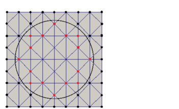
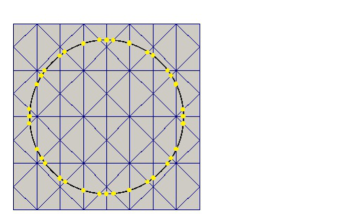
The fictitious domain for the fluid is considered on the whole domain $\mathcal{O}$. Let us introduce three discrete finite element spaces, $\tilde{\mathbf{V}}^{h}\subset\mathbf{H}^{1}(\mathcal{O})$, $\tilde{Q}^{h}\subset\mathrm{L}^{2}_{0}(\mathcal{O})$ and $\tilde{\mathbf{W}}^{h}\subset\mathbf{L}^{2}(\mathcal{O})$. Notice that the spaces $\mathbf{V},\ Q,\ \mathbf{W}$ introduced to define the weak formulation are included into those spaces defined all over the domain $\mathcal{O}=\mathcal{F}\cup\mathcal{S}$. In practice, $\mathcal{O}$ is a simple domain, so that the construction of a unique mesh for all spaces is straightforward (the interface between the fluid and the structure is not considered). Let us consider for instance a rectangular domain where a structured uniform mesh $\mathcal{T}^{h}$ can be constructed (see Figure 3). Classical finite element discretizations can be defined on the spaces $\tilde{\mathbf{V}}^{h}$, $\tilde{Q}^{h}$ and $\tilde{\mathbf{W}}^{h}$. For $\tilde{\mathbf{V}}^{h}$, let us consider for instance a subspace of the continuous functions $C(\overline{\mathcal{O}})$ defined by

$$\tilde{\mathbf{V}}^{h} = \left\{\boldsymbol{\mathrm{v}}^{h}\in C(\overline{\mathcal{O}})\mid\boldsymbol{\mathrm{v}}^{h}_{\left|\partial\mathcal{O}\right.}=0,\ \boldsymbol{\mathrm{v}}^{h}_{\left|T\right.}\in P(T),\ \forall T\in\mathcal{T}^{h}\right\},$$

where $P(T)$ is a finite dimensional space of regular functions, containing $P_{k}(T)$ the polynom space of degree less or equal to an integer $k$ ($k\geq 1$). For more details, see [30] for instance. The mesh step stands for $\displaystyle h=\max_{T\in\mathcal{T}^{h}}h_{T}$, where $h_{T}$ is the diameter of $T$. In order to split the fluid domain and the structure domain, we define spaces on the fluid part $\mathcal{F}$ and on the interface $\Gamma$ only, as

$$\mathbf{V}^{h}:=\tilde{\mathbf{V}}^{h}_{\left|\mathcal{F}\right.},\quad Q^{h}:=\tilde{Q}^{h}_{\left|\mathcal{F}\right.},\quad\mathbf{W}^{h}:=\tilde{\mathbf{W}}^{h}_{\left|\Gamma\right.}.$$

Figure 2: Illustration of the elements cut with respect to the level-set.

Notice that $\mathbf{V}^{h}$, $Q^{h}$, $\mathbf{W}^{h}$ are respective natural discretizations of $\mathbf{V}$, $Q$ and $\mathbf{W}$. It corresponds to cutting the basis functions of spaces $\tilde{\mathbf{V}}^{h}$, $Q^{h}$ and $\tilde{\mathbf{W}}^{h}$, as shown in Figure 2. This approach is equivalent to the eXtended Finite Element Method, as proposed in [13] or [12], where the standard finite element method basis functions are multiplied by Heaviside functions ($H({\bf x})=1$ for ${\bf x}\in\mathcal{F}$ and $H({\bf x})=0$ for ${\bf x}\in\mathcal{O}\setminus\mathcal{F}$), and the products are substituted in the variational formulation of the problem. Thus the degrees of freedom inside the fluid domain $\mathcal{F}$ are used in the same way as in the standard finite element method, whereas the degrees of freedom in the solid domain $\mathcal{S}$ at the vertexes of the elements cut by the interface (the so called virtual degrees of freedom) do not define the field variable at these nodes, but they are necessary to define the fields on $\mathcal{F}$ and to compute the integrals over $\mathcal{F}$. The remaining degrees of freedom, corresponding to the basis functions with support completely outside of the fluid, are eliminated (see Figure 3). We refer to the papers aforementioned for more details.

(a)                                                          (b)

Figure 3: Mesh on a fictitious domain. (a) Standard degrees of freedom (black, outside the disk), virtual ones (red, inside the disk), remaining ones are removed. (b) Bases nodes used for the multiplier space (yellow, on the disk).

The discrete problem consists in finding $(\boldsymbol{\mathrm{u}}^{h},p^{h},\boldsymbol{\mathrm{\lambda}}^{h},{\bf h}^{\prime},{\bf h},\theta^{\prime},\theta)\in\mathbf{V}^{h}\times Q^{h}\times\mathbf{W}^{h}\times\mathbb{R}^{2}\times\mathbb{R}^{2}\times\mathbb{R}\times\mathbb{R}$ such that

$$\left\{\begin{array}[]{lll}\displaystyle\int_{\mathcal{F}}\rho_{f}\frac{\partial{\bf u}^{h}}{\partial t}\cdot{\bf v^{h}}\mathrm{d}\mathcal{F}+\mathcal{A}(({\bf u}^{h},p^{h},{\boldsymbol{\mathrm{\lambda}}}^{h});{\bf v}^{h})+\int_{\mathcal{F}}\rho_{f}[({\bf u}^{h}\cdot\nabla){\bf u}^{h}]\cdot{\bf v}^{h}\mathrm{d}\mathcal{F}=\int_{\mathcal{F}}\rho_{f}{\bf g}\cdot{\bf v}^{h}\mathrm{d}\mathcal{F},\\ &\forall{\bf v}^{h}\in\mathbf{V}^{h},\\ &\\ \mathcal{B}(({\bf u}^{h},p^{h},{\boldsymbol{\mathrm{\lambda}}}^{h});q^{h})=0,&\forall q^{h}\in Q^{h},\\ &\\ \mathcal{C}(({\bf u}^{h},p^{h},{\boldsymbol{\mathrm{\lambda}}}^{h});{\boldsymbol{\mathrm{\mu}}}^{h})=\mathcal{G}({\boldsymbol{\mathrm{\mu}}}^{h}),&\forall{\boldsymbol{\mathrm{\mu}}}^{h}\in\mathbf{W}^{h},\\ &\\ \displaystyle m_{s}{\bf h}^{\prime\prime}(t)=-\int_{\partial\mathcal{S}(t)}{\boldsymbol{\mathrm{\lambda}}}^{h}\mathrm{d}\Gamma-m_{s}{\bf g},\qquad\displaystyle I\theta^{\prime\prime}(t)=-\int_{\partial\mathcal{S}(t)}({\bf x}-{\bf h}(t))^{\bot}\cdot{\boldsymbol{\mathrm{\lambda}}}^{h}\mathrm{d}\Gamma.&\\ \end{array}\right.$$

This is a system of nonlinear differential algebraic equations which can be formulated into a compact form. We denote by $\boldsymbol{U}$, $\boldsymbol{P}$ and $\boldsymbol{\Lambda}$ the respective degrees of freedom of $\boldsymbol{\mathrm{u}}^{h}$, $p^{h}$ and $\boldsymbol{\mathrm{\lambda}}^{h}$. After standard finite element discretization of the following bilinear forms

$$\mathcal{M}_{{\bf u}{\bf u}}:({\bf u},{\bf v}) \longmapsto \int_{\mathcal{F}}\rho_{f}{\bf u}.{\bf v}\mathrm{d}\mathcal{F},\qquad\mathcal{M}_{\boldsymbol{\mathrm{\lambda}}}:{\boldsymbol{\mathrm{\lambda}}}\longmapsto-\int_{\partial\mathcal{S}(t)}{\boldsymbol{\mathrm{\lambda}}}\mathrm{d}\Gamma,$$

$$\mathcal{A}_{{\bf u}{\bf u}}:({\bf u},{\bf v}) \longmapsto 2\nu\int_{\mathcal{F}}D({\bf u}):D({\bf v})\mathrm{d}\mathcal{F}-4\nu^{2}\gamma\int_{\Gamma}\left(D({\bf u})\boldsymbol{\mathrm{n}}\right)\cdot\left(D({\bf v})\boldsymbol{\mathrm{n}}\right)\mathrm{d}\Gamma,$$

$$\mathcal{A}_{{\bf u}p}:({\bf v},p) \longmapsto -\int_{\mathcal{F}}p\mathrm{div}\ {\bf v}\mathrm{d}\mathcal{F}+2\nu\gamma\int_{\Gamma}p\left(D({\bf v})\boldsymbol{\mathrm{n}}\cdot\boldsymbol{\mathrm{n}}\right)\mathrm{d}\Gamma,$$

$$\mathcal{A}_{{\bf u}{\boldsymbol{\mathrm{\lambda}}}}:({\bf u},{\boldsymbol{\mathrm{\lambda}}}) \longmapsto -\int_{\Gamma}{\boldsymbol{\mathrm{\lambda}}}\cdot{\bf v}\mathrm{d}\Gamma+2\nu\gamma\int_{\Gamma}{\boldsymbol{\mathrm{\lambda}}}\cdot\left(D({\bf v})\boldsymbol{\mathrm{n}}\right)\mathrm{d}\Gamma,$$

$$\mathcal{A}_{pp}:(p,q) \longmapsto -\gamma\int_{\Gamma}pq\mathrm{d}\Gamma,\hskip 14.22636pt\mathcal{A}_{p{\boldsymbol{\mathrm{\lambda}}}}:(q,{\boldsymbol{\mathrm{\lambda}}})\longmapsto-\gamma\int_{\Gamma}q{\boldsymbol{\mathrm{\lambda}}}\cdot\boldsymbol{\mathrm{n}}\mathrm{d}\Gamma,$$

$$\mathcal{A}_{{\boldsymbol{\mathrm{\lambda}}}{\boldsymbol{\mathrm{\lambda}}}}:({\boldsymbol{\mathrm{\lambda}}},{\boldsymbol{\mathrm{\mu}}}) \longmapsto -\gamma\int_{\Gamma}{\boldsymbol{\mathrm{\lambda}}}\cdot{\boldsymbol{\mathrm{\mu}}}\mathrm{d}\Gamma,$$

we define matrices like $M_{{\bf u}{\bf u}}$ from $\mathcal{M}_{{\bf u}{\bf u}}$, etc…, the vector $\boldsymbol{G}$ from $\mathcal{G}$, ${\bf F}$ from the gravity forces $\rho_{f}{\bf g}$, $M_{\boldsymbol{\mathrm{\lambda}}}$ the matrix computed by integration over $\Gamma$ of the $\mathbf{W}^{h}$ basis functions and $N(\boldsymbol{U}(t))\boldsymbol{U}(t)$ the matrix depending on the velocity and corresponding to the nonlinear convective term $\displaystyle\int_{\mathcal{F}}\rho_{f}[({\bf u}\cdot\nabla){\bf u}]\cdot{\bf v}\mathrm{d}\mathcal{F}$. Then the matrix formulation is given by

$$M_{{\bf u}{\bf u}}\frac{\mbox{d}\boldsymbol{U(t)}}{\mbox{d}t}+A_{{\bf u}{\bf u}}\boldsymbol{U}(t)+N(\boldsymbol{U}(t))\boldsymbol{U}(t)+A_{{\bf u}p}\boldsymbol{P}(t)+A_{{\bf u}{\bf\lambda}}\boldsymbol{\Lambda}(t)={\bf F},$$ (7)

$$A^{T}_{{\bf u}p}\boldsymbol{U}(t)+A_{pp}\boldsymbol{P}(t)+A_{p{\bf\lambda}}\boldsymbol{\Lambda}(t)=0,$$ (8)

$$A^{T}_{{\bf u}{\bf\lambda}}\boldsymbol{U}(t)+A^{T}_{p{\bf\lambda}}\boldsymbol{P}(t)+A_{{\bf\lambda}{\bf\lambda}}\boldsymbol{\Lambda}(t)=\boldsymbol{G},$$ (9)

$$\displaystyle m_{s}{\bf h}^{\prime\prime}(t)=M_{\bf\lambda}\boldsymbol{\Lambda}(t)-m_{s}{\bf g},$$ (10)

$$\displaystyle\text{{$I\theta^{\prime\prime}(t)=M_{\bf\lambda}\left[({\bf x}-{\bf h}(t))^{\bot}\cdot\boldsymbol{\Lambda}(t)\right]$}}.$$ (11)

At the interface $\Gamma=\partial\mathcal{S}(t)$ represented by a level-set function which cuts the global mesh, the coupling between the fluid and the structure is imposed by a Dirichlet condition whose elements are determined through the computation of $\sigma(\boldsymbol{\mathrm{u}},p){\bf n}$. The main advantage of our numerical method - mathematically justified in [21] - is to return an optimal approximation $\boldsymbol{\Lambda}(t)$ of $\sigma(\boldsymbol{\mathrm{u}},p){\bf n}$ at the interface. Getting a good approximation of this quantity is crucial for the dynamics of the system.

3.2 Time discretization and treatment of the nonlinearity

Classical methods like $\theta$-methods can be used for the time discretization. For a matter of unconditional stability of the scheme, we consider an implicit discretization based on the backward Euler method. We denote by $\boldsymbol{U}^{n+1}$ the solution at the time level $t^{n+1}$ and $dt=t^{n+1}-t^{n}$ is the time step. Particular attention must be done for a moving particle problem. Indeed, at the time level $t^{n+1}$ the solid occupies $\mathcal{S}(t^{n+1})$ which is different from the previous time level $t^{n}$. So, the field variable at the time level $t^{n+1}$ can become undefined near the interface since there was no fluid flow at the time level $t^{n}$ ($\mathcal{S}(t^{n+1})\neq\mathcal{S}(t^{n})$ for the solid and $\mathcal{F}(t^{n+1})\neq\mathcal{F}(t^{n})$ for the fluid). In other words, some degrees of freedom for the fluid part which are not considered at the time level $t^{n}$ must be taken into account at the time level $t^{n+1}$. In particular, the velocity field must be known in such nodes. In the present work, we impose the velocity to be equal to the motion of the solid. The validity of this approximation is justified as soon as time step is sufficiently small to ensure that the structure moves progressively across the mesh without jump of cells (when the level-set doesn’t cuts this cell). This constraint is not too strong and corresponds to the classical CFL condition for velocity of the structure.
In the following we present the algorithm we perform to compute at the time level $t^{n+1}$ the solution ($\boldsymbol{U}^{n+1},\boldsymbol{P}^{n+1},\boldsymbol{\Lambda}^{n+1},{\bf h}^{\prime n+1},{\bf h}^{n+1},\theta^{\prime n+1},\theta^{n+1}$) on $\mathcal{F}(t^{n+1})$. To simplify, we assume that $dt$ is constant. At the time level $t^{n}$ we have access to ($\boldsymbol{U}^{n},\boldsymbol{P}^{n},\boldsymbol{\Lambda}^{n},{\bf h}^{\prime n},{\bf h}^{n},\theta^{\prime n},\theta^{n}$) on $\mathcal{F}(t^{n})$.

• Velocity of the structure -From $\boldsymbol{\Lambda}^{n}$, we compute $({\bf h}^{\prime n+1},\theta^{\prime n+1})$ using (10) and (11) with the mid-point method, as

  $$\displaystyle m_{s}\frac{{\bf h}^{\prime n+1}-{\bf h}^{\prime n}}{dt}=M_{\bf\lambda}\boldsymbol{\Lambda}^{n}-m_{s}{\bf g},$$

  $$\displaystyle I\frac{\theta^{\prime n+1}-\theta^{\prime n}}{dt}=M_{\bf\lambda}\left[({\bf x}-{\bf h}^{n})^{\bot}\cdot\boldsymbol{\Lambda}^{n}\right].$$

• Position of the structure - From $\boldsymbol{\Lambda}^{n}$, we compute $({\bf h}^{n+1},\theta^{n+1})$ using (10) and (11) with mid point rule

  $$\displaystyle m_{s}\frac{{\bf h}^{n+1}-2{\bf h}^{n}+{\bf h}^{n-1}}{dt^{2}}=M_{\bf\lambda}\boldsymbol{\Lambda}^{n}-m_{s}{\bf g},$$

  $$\displaystyle I\frac{\theta^{n+1}-2\theta^{n}+\theta^{n-1}}{dt^{2}}=M_{\bf\lambda}\left[({\bf x}-{\bf h}^{n})^{\bot}\cdot\boldsymbol{\Lambda}^{n}\right].$$

• We update the geometry to determine $\mathcal{F}(t^{n+1})$. It corresponds to update the position of the level-set which is defined from ${\bf h}^{n+1}$ and $\theta^{n+1}$.

• We complete the velocity $\boldsymbol{U}^{n}$ defined on $\mathcal{F}(t^{n})$ to the full domain $\mathcal{O}$ by imposing the velocity on each node of $\mathcal{S}(t^{n+1})$ to be equal to ${\bf h}^{\prime n+1}+\theta^{\prime n+1}({\bf x}-{\bf h}^{n+1})^{\bot}$.
  After this step, we know the Dirichlet condition for the velocity to impose at the interface $\Gamma(t^{n+1})=\partial\mathcal{S}(t^{n+1})$. So we determine $\boldsymbol{G}^{n+1}$ in (9) from ${\bf u}_{\Gamma}^{n+1}={\bf h}^{\prime n+1}+\theta^{\prime n+1}({\bf x}-{\bf h}^{n+1})^{\bot}$.

• Finally, we compute $(\boldsymbol{U}^{n+1},\boldsymbol{P}^{n+1},\boldsymbol{\Lambda}^{n+1})$ such that

  $$M_{{\bf u}{\bf u}}\frac{\boldsymbol{U}^{n+1}-\boldsymbol{U}^{n}}{dt}+A_{{\bf u}{\bf u}}\boldsymbol{U}^{n+1}+N(\boldsymbol{U}^{n+1})\boldsymbol{U}^{n+1}+A_{{\bf u}p}\boldsymbol{P}^{n+1}+A_{{\bf u}{\bf\lambda}}\boldsymbol{\Lambda}^{n+1}=\boldsymbol{F}^{n+1},$$

  $$A^{T}_{{\bf u}p}\boldsymbol{U}^{n+1}+A_{pp}\boldsymbol{P}^{n+1}+A_{p{\bf\lambda}}\boldsymbol{\Lambda}^{n+1}=0,$$

  $$A^{T}_{{\bf u}{\bf\lambda}}\boldsymbol{U}^{n+1}+A^{T}_{p{\bf\lambda}}\boldsymbol{P}^{n+1}+A_{{\bf\lambda}{\bf\lambda}}\boldsymbol{\Lambda}^{n+1}=\boldsymbol{G}^{n+1}.$$

  At this stage, the solution of the resulting nonlinear algebraic system is achieved by a Newton method. The initialization of the Newton algorithm is done with the solution at the previous time step (this solution is defined in item 4–).

• We complete the velocity $\boldsymbol{U}^{n+1}$ defined on $\mathcal{F}(t^{n+1})$ to the full domain $\mathcal{O}$ by imposing the velocity on each node of $\mathcal{S}(t^{n+1})$ to be equal to ${\bf h}^{\prime n+1}+\theta^{\prime n+1}({\bf x}-{\bf h}^{n+1})^{\bot}$.

Remark 1: In practice the mid-point method is used to update the geometry of the structure for the computation of ${\bf h}^{\prime n+1},{\bf h}^{n+1},{\theta^{\prime}}^{n+1},\theta^{n+1}$.
Remark 2: Step 6– plays an important role to update the geometry. Indeed, after extension, we have access to the values of the solution at each node of the full domain. Thus new nodes that appear after update have some values and no interpolation is required.

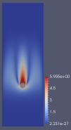
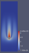
4 Numerical tests: Free fall of a disk in a channel

For validation of our method, we consider the numerical simulation of the motion of a disk falling inside an incompressible Newtonian viscous fluid. The parameters used in the computation, for a disk of radius $R=0.125$ cm in a channel of dimension $[0,2]\times[0,6]$, are given in Table 1.

Parameter	$\rho_{f}$	$\rho_{s}$	$\nu$	$g$
Unit	g/cm2	g/cm2	g/cm2 s	cm/s2
value	1	1.25	0.1	981

Table 1: Parameters used for the simulation.

This simulation is well documented in the literature and considered as a challenging benchmark. We refer to the paper [7] where fictitious domain method is used and [31] for simulations with mesh adaptation.
For the finite element discretization, we consider classical Lagrange family with $P_{2}-P_{1}-P_{0}$ for respectively ${\bf u}$, $p$, and $\boldsymbol{\lambda}$ , which is a choice that satisfies the inf-sup condition required for such kind of problems (see [21] for more details). Uniform triangular meshes are used and defined by imposing a uniform repartition of points on the boundary of the domain. Two meshes are used, $mesh_{50\times 150}$ with $50$ points in $x$-direction and $150$ points in $y$-direction, and $mesh_{100\times 300}$ with $100$ points in $x$-direction and $300$ points in $y$-direction.
Numerical tests are performed with and without stabilization to underline the advantage of the method. When stabilization is considered, we choose $\gamma=h\times\gamma_{0}$ where $\gamma_{0}=0.05$ (see [21] for the justification of this choice). The parameter $\gamma$ has to obey to a compromise between the coerciveness of the system and the weight of the stabilization term. The time discretization step $dt$ is initialized to $0.0005$ and adapted at each time iteration to satisfy a CFL condition. More precisely, we evaluate the norm of the velocity at each point of the structure and we deduce the maximum value $v_{m}=\max_{{\bf x}\in\mathcal{S}(t^{n})}(\|\boldsymbol{\mathrm{u}}({\bf x})\|)$. Then we impose $dt=\min(0.9h/v_{m},2h^{2}/{\nu})$. This condition is not restrictive and we observe that $dt\in[0.0005;0.006]$ in all the tests.
In the literature, in order to study the fall of the disk, curves are given to show the evolution of the vertical velocity and the position of the center of the disk according to the time. We present the same analysis for different adaptation of our method. As expected, the disk reaches quickly a uniform fall velocity with slight moving on the right side of the vertical symmetry axis. This observation was already reported in the literature and is not specific to our method. One challenge is to propose robust methods that limit this breaking. In this section, we show that our method gives an answer to this question. Indeed, numerical simulations can be done with coarse meshes, even if it is not recommended with a fictitious domain approach (points on the interface can be far from the degrees of freedom introduced by the finite element method).

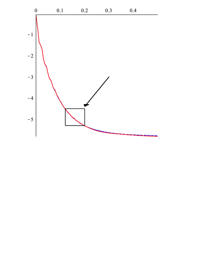
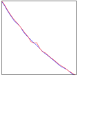
Contribution of the stabilization technique: Numerical tests are performed with the mesh $mesh_{50\times 150}$, with and without performing the stabilization ($\gamma_{0}=0$). We compute the position of the disk according to the time and represent separately the vertical and horizontal positions.
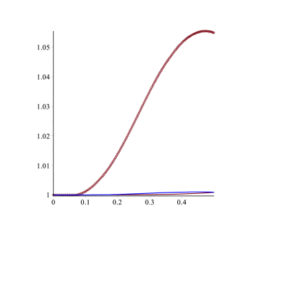
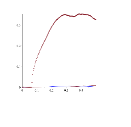
In Figure 4 we represent the vertical velocity through the time. The results are similar, whether we perform stabilization or not. However, with the stabilization technique the method is more robust. If we zoom in (see Figure 4), without stabilization (red curve) some perturbations appear. When we compare the positions of the disk through the time, we do not observe difference on the vertical position in the Figure 5(a). However the difference is more important for the horizontal position and the rotation of the disk. The curves are plotted in red in Figure 6, with the mesh $mesh_{50\times 150}$. With the stabilization technique the results are clearly improved. Without stabilization, the symmetry is broken even if it seems that the disk comes back around the symmetry axis of the cavity at the end of the simulation. This behavior related to the computation of the angular velocity which is represented in Figure 6(b).

Figure 4: Evolution in time $t\in[0;0.5]$ of the vertical velocity for $mesh_{50\times 150}$ with stabilization in blue color and without stabilization in red color.

Influence of the mesh size: With stabilization, we compare the simulations obtained with $mesh_{50\times 150}$ and $mesh_{100\times 300}$. The results are given in Figure 5 (red curves for $mesh_{50\times 150}$ and blue curves for $mesh_{100\times 300}$). As expected, the smoothness of the solution is better when a sharper mesh is used. Besides, the result seems to be as good as results obtained in [7, 31] for instance. When a coarse mesh is used, the velocity is over-estimated. This observation can be justified by the capability of the method for preserving the conservation of the mass. Indeed, with a coarse mesh, a numerical added mass appears in the system. This artificial mass is proportional to the stabilization terms (see $\mathcal{A}_{p{\boldsymbol{\mathrm{\lambda}}}}$ and $\mathcal{A}_{{\boldsymbol{\mathrm{\lambda}}}{\boldsymbol{\mathrm{\lambda}}}}$ in the discrete problem) which are themselves proportional to the mesh size, and thus it can be neglected when the mesh size decreases.

(a)                                                              (b)

Figure 5: Simulations for $t\in[0;0.5]$, for $mesh_{50\times 150}$ in red color, and for $mesh_{100\times 300}$ in blue color. (a) Vertical position of the disk, (b) Vertical velocity.

The computation of the horizontal position of the disk is given in Figure 6(a). We observe that the disk tends to come back towards the symmetry axis of the cavity atthe end of the simulation with $mesh_{100\times 300}$, unlike in the simulations with $mesh_{50\times 150}$, where the symmetry breaking seems to growth. This phenomena can be observed in Figure 6(b) which represents the evolution of the rotation angle of the disk. With $mesh_{50\times 150}$ this angle always growths, unlike for the sharper mesh $mesh_{100\times 300}$. This behavior can be justified by perturbation associated with our numerical method, in particular for the treatment of the nonlinear term. Moreover, a perturbation in horizontal velocity component is difficult to compensate during the simulation and contributes to the amplifying the phenomena. However, with stabilization, relevant values of the rotation are obtained and show that their influence is reduced compared with the translation.

(a)                                                              (b)

Figure 6: Simulations depending on time $t\in[0;0.5]$ with stabilization for $mesh_{50\times 150}$ red lines and for $mesh_{100\times 300}$ blue lines. Red curves (upper) with points have no stabilization with $mesh_{50\times 150}$ points. (a) Horizontal position, (b) Rotation angle.

Figure 7: Imagery illustration of the intensity of the fluid’s velocity during the fall of the ball.

5 Practical remarks on the numerical implementation.

• All the numerical simulations were performed with the free generic library Getfem++ [32] (same source code for 2D and 3D) and implemented on High Performing Computers (parallel computations).

• In order to compute properly the integrals over elements at the interface (during assembling procedure), external call to Qhull Library [33] is realized.

• In the algorithm, steps 1– and 2– require computing of $M_{\bf\lambda}\boldsymbol{\Lambda}^{n}$ and $M_{\bf\lambda}\left[({\bf x}-{\bf h}^{n})^{\bot}\cdot\boldsymbol{\Lambda}^{n}\right]$, corresponding to integrations over the level-set. Such integrations require particular attention, in the sake of preserving a good accuracy. Indeed, the integrations must use nodes on level-set and accurate values on that nodes are required (no interpolation).

• The method is very efficient in time computation, since it requires an update of the assembling matrices only locally near the interface.

• As mentioned in [14], it is possible to define a reinforced stabilization technique in order to prevent difficulties that can occur when the intersection of the solid and the mesh over the whole domain introduce "very small" elements. The technique consists in selecting elements which are better to deduce the normal derivative on $\Gamma$. A similar approach is given in [34]. We think that this kind of reinforced stabilization technique can prevent the perturbations that appear during simulation (see zoom in Figure 4).

6 Conclusion

In this paper, we have considered a new fictitious domain method based on the extended finite element with stabilized term applied to the Navier-Stokes equations coupled with a moving solid. This method is quite simple to implement since all the variables (multipliers and primal variables) are defined on a single mesh independent of the computational domain. The algorithm leads to a robust method (good computation of the normal Cauchy stress tensor) whatever is the intersection of the domain with the - not necessarily sharp - mesh. The simulation of a falling disk with respect to the time confirms that our approach is able to predict well the interaction between the fluid and the structure. The stabilization must be considered to obtain more physical results preserving symmetry. Applications in 3D are in progress, in particular for control flow by acting on the boundary of the solid.