DISCOVERY OF A FAINT OUTER HALO MILKY WAY STAR CLUSTER IN THE SOUTHERN SKY
Abstract
We report the discovery of a new, low luminosity star cluster in the outer halo of the Milky Way. High quality photometry is presented, from which a color-magnitude diagram is constructed, and estimates of age, [Fe/H], [/Fe], and distance are derived. The star cluster, which we designate as Kim 2, lies at a heliocentric distance of kpc. With a half-light radius of pc and ellipticity of , it shares the properties of outer halo GCs, except for the higher metallicity ([Fe/H]) and lower luminosity (. These parameters are similar to those for the globular cluster AM 4, that is considered to be associated with the Sagittarius dwarf spheroidal galaxy. We find evidence of dynamical mass segregation and the presence of extra-tidal stars that suggests Kim 2 is most likely a star cluster. Spectroscopic observations for radial-velocity membership and chemical abundance measurements are needed to further understand the nature of the object.
Subject headings:
globular clusters: general — Galaxy: formation – Galaxy: halo – galaxies: dwarf — Local Group1. Introduction
Globular clusters in the outer halo of the Milky Way (MW) hold important clues to the formation and structure of their host galaxy. Most of these rare distant globular clusters exhibit anomalously red horizontal branch morphology at given metal abundance (Lee1994), and belong to the so-called “young halo” system (Zinn1993a). Young halo objects are hypothesized to have formed in external dwarf galaxies that were accreted into the Galactic potential well and disrupted by the Galactic tidal force (Searle1978). This scenario has received considerable support by observational results from the MW and M31 (DaCosta1995; Marin-Franch2009; Mackey2004; Mackey2010). Indeed, the young halo clusters resemble the globular clusters located in dwarf galaxies associated with the Milky Way in terms of horizontal branch type (Zinn1993b; Smith1998; Johnson1999; Harbeck2001) and other properties such as luminosity, age, and chemical abundance (DaCosta2003).
Despite the significant contribution of modern imaging surveys like the Sloan Digital Sky Survey (Ahn2014) to the discoveries of new Milky Way satellite galaxies (e.g Willman2005; Belokurov2007; Irwin2007; Walsh2007) and extended substructures(e.g Newberg2003; Grillmair2009), only a small number of star clusters have been discovered (Koposov2007; Belokurov2010; Balbinot2013; Kim1), and these are typically located in the inner halo of the Milky Way. A new distant MW halo object at 145 kpc, by the name of PSO J174.0675-10.8774, or Crater, was recently discovered simultaneously in two independent surveys (Laevens2014; Belokurov2014). Although this stellar system shares the structural properties of globular clusters in the outer halo of the Galaxy, confirming its true nature still requires additional investigation. Other than PSO J174.0675-10.8774, only six known Milky Way GCs are located at Galactocentric distances larger than 50 kpc, namely AM 1, Eridanus, NGC 2419, Palomar 3, 4, and 14 (see Table 1). The Hubble Space Telescope Advanced Camera for Survey photometry of the Galactic GCs (Sarajedini2007; Dotter2011) has confirmed that all of the outer halo GCs except for NGC 2419 have a red horizontal branch and young ages relative to the inner halo GCs (Dotter2010).
| PSO J174.0675 | ||||||||
|---|---|---|---|---|---|---|---|---|
| Parameter | AM 1 | Pal 3 | Pal 4 | Pal 14 | Eridanus | NGC2419 | -10.8774aaPSO J174.0675-10.8774 is not yet unambiguously confirmed as a globular cluster. | Unit |
| 03 55 02.3 | 10 05 31.9 | 11 29 16.8 | 16 11 00.6 | 04 24 44.5 | 07 38 08.4 | 11 36 16.2 | h:m:s | |
| 49 36 55 | 00 04 18 | 28 58 25 | 14 57 28 | 21 11 13 | 38 52 57 | 10 52 39 | ||
| 258.34 | 240.15 | 202.31 | 28.74 | 218.10 | 180.37 | deg | ||
| deg | ||||||||
| 123.3 | 92.5 | 108.7 | 76.5 | 90.1 | 82.6 | 145 | kpc | |
| 124.6 | 95.7 | 111.2 | 71.6 | 95.0 | 89.9 | 145 | kpc | |
| [Fe/H] | dex | |||||||
| (Plummer) | 15.2 | 18.0 | 16.6 | 28.0 | 12.4 | 22.1 | 22 | pc |
| mag |
Note. — From Harris1996, combined with Laevens2014 for PSO J174.0675-10.8774.
In this paper, we report the discovery of a distant globular cluster in the constellation of Indus. This object was first detected in our on-going southern sky blind survey with the Dark Energy Camera (DECam) at the 4 m Blanco Telescope at Cerro Tololo Inter-American Observatory (CTIO) and confirmed with deep GMOS-S images at the 8.1 m Gemini South telescope on Cerro Pachõn, Chile (Section 2 & 3). The new star cluster, which we designate as Kim 2, is at a distance kpc and has a low luminosity of only mag and a metallicity of [Fe/H], slightly higher than the other young halo clusters (Section 4). In section 5 we discuss the implication of these properties, present evidence for mass segregation in the cluster and discuss its possible origin.
| Filter | UT Date | Exposure | Seeing | Airmass |
|---|---|---|---|---|
| Sep 20 2014 | s | - | 1.08 - 1.12 | |
| Oct 29 2014 | s | - | 1.23 - 1.42 |
2. Discovery
As part of the Stromlo Milky Way Satellite Survey111http://www.mso.anu.edu.au/jerjen/SMS_Survey.html we collected imaging data for 500 sqr deg with the DECam at the 4 m Blanco telescope at CTIO over three photometric nights from 17th to 19th July 2014. DECam is an array of sixty-two 2k4k CCD detectors with a 2.2 deg2 field of view and a pixel scale of (unbinned). We obtained a series of s dithered exposures in the and band under photometric conditions. The average seeing was for both filters each night. The stacked images were reduced via the DECam community pipeline (DECamCP2014). We used WeightWatcher (WeightWatcher) for weight map combination and SExtractor (SExtractor) for source detection and photometry. Sources were morphologically classified as stellar or non-stellar objects. For the photometric calibration, we regularly observed Stripe 82222 http://cas.sdss.org/stripe82/en/ of the Sloan Digital Sky Survey throughout the three nights with 50 s single exposures in each band. To determine zero points and color terms, we matched our instrumental magnitudes with the Stripe 82 stellar catalogue to a depth of 23 mag and fit the following equations:
| (1) |
| (2) |
where and are the zero points, and are the respective color terms, and are the first order extinctions, and is the mean airmass.
In the Stripe 82 images we observed right after the Kim 2 field, we found 399 stars with and in the identical CCD chip where the cluster was detected. We restricted the calibration to stars fainter than mag to avoid the saturation limit of our DECam data. We determined the zero points, color terms and associated uncertainties by bootstrapping with replacements performed 1000 times and using a linear least-squares fit with 3-sigma clipping rejection. Uncertainties in the zero points were measured 0.013 mag in and 0.010 in , whereas uncertainties in the color terms are 0.011 and 0.009, respectively. The most recent extinction values and for CTIO were obtained from the Dark Energy Survey team. We calibrated our DECam photometry of the Kim 2 field using these coefficients and corrected for exposure time differences.
We employ the same detection algorithm as described in Kim1 to search the photometry catalog for stellar overdensities. In essence, we apply a photometric filter in color-magnitude space adopting isochrone masks based on the Dartmouth stellar evolution models (Dartmouth) to enhance the presence of old and metal-poor stellar populations relative to the Milky Way foreground stars. We then bin the R.A., decl. positions of the stars and convolve the 2-D histogram with a Gaussian kernel. The statistical significance of potential overdensities is measured by comparing their signal to noise ratios (S/Ns) on the density map to those of random clustering in the residual Galactic foreground. This process is repeated for different bin sizes and Gaussian kernels by shifting the isochrone masks over a range of distance moduli from 16 to 22 magnitudes. We detected the new stellar overdensity with a significance of relative to the Poisson noise of the Galactic foreground stars. This object that we chose to call Kim 2 was found at 21h08m49.97s, 51d09m48.6s(J2000) in the constellation of Indus.
3. Follow-up Observations and Data Reduction
To investigate the nature of Kim 2, deep follow-up observations were obtained with the Gemini Multi-Object Spectrograph in imaging mode at the 8.1 m Gemini South telescope through director’s time (GS-2014B-DD-3) on Sep 20, 21, 22, 30 and Oct 29. Since June 2014, GMOS-S is equipped with a new array of three pixel2 Hamamatsu CCDs with a field of view and a pixel scale of (unbinned). To reduce readout time, we employed binning, resulting in a plate scale of pixel-1. A series of s dithered exposures in and in band were observed. These and filters are similar, but not identical, to the and filters used by the SDSS. We chose the nine best images in each band for our photometric analysis. A summary of the selected observations is presented in Table 2.
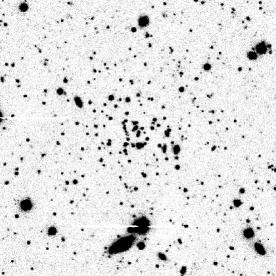
We employed the latest Gemini IRAF package V1.13 (commissioning release)333http://www.gemini.edu/node/12227 for data reduction. We applied bias and flat-field images provided by the Gemini science archive for standard GMOS baseline calibration to each exposure using the GIREDUCE task. The three CCD frames of each reduced image were then mosaicked into a single frame using the GMOSAIC task. Figure 1 shows a cut out at the centre of a deep band image, formed by combining the nine individual mosaicked frames of the passband using the IMCOADD task, in which Kim 2 is visible as a concentration of faint stars.
The photometry of the reduced GMOS images was carried out using the software package kitchen_sync presented in Anderson2008 and modified to work with GMOS-S data. It exploits two distinct methods to measure bright and faint stars. Astrometric and photometric measurements of bright stars have been performed in each mosaicked image, independently, by using appropriate point-spread function (PSF) model, and later combined. To derive the PSF models, we adapted to our data the software as described in (Anderson2006, see also Bellini2010). Briefly, we used the most isolated, bright and non-saturated stars in each image to determine a grid of four empirical PSFs. To account for the spatial variation of the PSF across the field of view, we assumed that to each pixel of the image corresponds a PSF that is a bi-linear weighted interpolation of the closest four PSFs of the grid.
Furthermore, the flux and position can also be determined by fitting for each star simultaneously all the pixels in all the exposures. This approach works better for very faint stars, which can not be robustly measured in every individual exposure. We refer the reader to the papers by Anderson2006 and Anderson2008 for further details.
We then conducted the photometric calibration using 65 stars with and we found in the field of view of GMOS. Comparing their instrumental magnitudes to the calibrated magnitudes of our DECam photometry in Section 2, we derived a calibration equation composed of a photometric zero point and a color term from bootstrapping the data 1000 times and performing a least-square fit with 3-sigma clipping rejection. Uncertainties in the zero points are 0.022 mag in the band and 0.023 mag in . Uncertainties in the color terms are 0.020 and 0.019, respectively.
We performed artificial star tests to determine the completeness level of our photometry. To do this we used the recipe and the software described in detail by Anderson2008. Briefly, we first generated an input list of artificial stars and placed along the fiducial line of the MS and the RGB of Kim 2, which we have derived by hand. The list includes the coordinates of the stars in the reference frame and the magnitudes in g and r bands. Artificial stars have been placed in each image according to the overall cluster distribution as in Milone2009.
For each star in the input list, the software by Anderson2008 adds, in each image, a star with appropriate flux and position and measures it by using the same procedure as for real stars. An artificial star is considered to be detected when the input and the output position differ by less then 0.5 pixel and the input and the output flux by less than 0.75 mag.
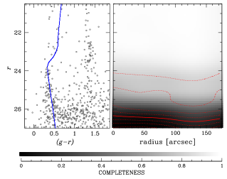
The software provides for artificial stars the same diagnostics of the photometric quality as for real star. We applied the same procedure used for real stars to select a sub-sample of stars with small astrometric errors, and well fitted by the PSF. Figure 2 shows the recovery rate of the input stars as a function of the stellar magnitude and the radial distance from the cluster center.
To address the effect of crowding, we measured the completeness not only as a function of the stellar magnitude but also the distance from the cluster center. For the latter, we divided the GMOS field into five concentric annuli, in each of which we measured the completeness in seven magnitude bins, in the interval . Interpolating the recovery rate of the input stars at each of these grid points allows us to estimate the completeness of any star at any position within the cluster as shown in Figure 2.
4. Candidate Properties
4.1. Color-Magnitude Diagram
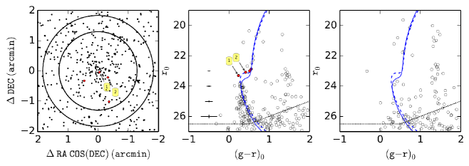
The left panel of Figure 3 shows the RA-DEC distribution of all objects classified as point source by our GMOS photometry centred on Kim 2. The middle panel of Figure 3 shows the extinction-corrected CMD of all stars located within () from the overdensity center. All magnitudes are individually corrected for Galactic reddening by the Schlegel1998 maps and the extinction coefficients of Schlafly2011. In Table LABEL:tab:GMOSdata, we present our GMOS photometry of all stars brighter than the 50% completeness level, the dotted line in the middle panel of Figure 3. For comparison, the right panel shows the CMD of stars in an equal area between the radii and , the majority of which are expected to be MW field stars.
The subgiant branch and the red giant branch (RGB) of this loose and faint cluster is almost absent, and no hints of an horizontal branch or red giant clump are visible. The main sequence (MS) however is well defined down to , below which our photometry is affected by incompleteness. There are four possible subgiant branch and MS turn-off stars (red dots in Figure 3) consistent with the location of a main-sequence that runs from mag down to mag. The stars labelled #1 and #2 have small angular distances from the nominal cluster center (see left panel of Figure 3). This supports the idea that they are cluster members. If true, we would observe a lack of stars between star #1 and the brightest main sequence stars. Such a gap in the luminosity function is uncommon but not unheard of, for example in Segue 3 (see Fig.2 in Fadely2011). Overplotted on our CMD are two theoretical isochrones from the Dartmouth data base. They will be discussed in the next section.
| Radial | Radial | |||||||||
|---|---|---|---|---|---|---|---|---|---|---|
| (J2000) | (J2000) | Distance | (J2000) | (J2000) | Distance | |||||
| (h m s) | ( ) | () | (mag) | (mag) | (h m s) | ( ) | () | (mag) | (mag) | |
| 21:08:49.81 | -51:09:46.66 | 0.040 | 24.16 | 0.37 | 21:08:46.11 | -51:09:52.80 | 0.608 | 24.86 | 1.18 | |
| 21:08:50.04 | -51:09:51.57 | 0.051 | 24.42 | 0.46 | 21:08:53.28 | -51:10:08.69 | 0.618 | 23.31 | 1.52 | |
| 21:08:49.78 | -51:09:51.74 | 0.060 | 21.70 | 1.34 | 21:08:51.43 | -51:09:13.99 | 0.620 | 25.80 | 0.36 | |
| 21:08:49.68 | -51:09:51.33 | 0.064 | 23.38 | 0.27 | 21:08:47.67 | -51:09:18.26 | 0.621 | 26.35 | 0.52 | |
| 21:08:50.42 | -51:09:51.05 | 0.082 | 23.83 | 0.32 | 21:08:46.14 | -51:09:35.97 | 0.636 | 25.28 | 0.29 | |
| 21:08:49.46 | -51:09:50.63 | 0.087 | 24.96 | 0.37 | 21:08:45.87 | -51:09:39.90 | 0.658 | 25.83 | 0.55 | |
| 21:08:49.50 | -51:09:45.45 | 0.090 | 26.27 | 0.52 | 21:08:46.96 | -51:09:20.73 | 0.662 | 23.46 | 1.54 | |
| 21:08:49.36 | -51:09:48.45 | 0.095 | 24.18 | 0.38 | 21:08:53.62 | -51:09:26.57 | 0.681 | 21.15 | 0.88 | |
| 21:08:49.61 | -51:09:43.60 | 0.100 | 24.71 | 0.40 | 21:08:47.79 | -51:09:13.09 | 0.683 | 26.09 | 0.31 | |
| 21:08:50.46 | -51:09:43.76 | 0.111 | 25.22 | 0.42 | 21:08:48.20 | -51:10:26.09 | 0.683 | 26.14 | 0.54 | |
| 21:08:50.45 | -51:09:53.91 | 0.117 | 23.97 | 0.35 | 21:08:53.07 | -51:10:17.52 | 0.685 | 25.48 | 0.50 | |
| 21:08:49.99 | -51:09:41.23 | 0.123 | 24.12 | 0.39 | 21:08:50.20 | -51:09:07.17 | 0.691 | 25.85 | 0.51 | |
| 21:08:50.48 | -51:09:42.44 | 0.130 | 25.52 | 0.61 | 21:08:50.17 | -51:10:30.25 | 0.695 | 20.67 | 1.36 | |
| 21:08:50.39 | -51:09:55.39 | 0.131 | 25.50 | 0.49 | 21:08:54.46 | -51:09:55.98 | 0.715 | 25.08 | 0.32 | |
| 21:08:50.52 | -51:09:41.00 | 0.154 | 24.94 | 0.37 | 21:08:49.22 | -51:09:05.58 | 0.727 | 25.98 | 0.54 | |
| 21:08:49.12 | -51:09:43.51 | 0.158 | 23.91 | 0.30 | 21:08:54.43 | -51:09:31.98 | 0.752 | 25.52 | 0.23 | |
| 21:08:50.41 | -51:09:40.04 | 0.158 | 24.81 | 0.43 | 21:08:50.76 | -51:10:33.49 | 0.758 | 25.60 | 0.47 | |
| 21:08:50.23 | -51:09:58.76 | 0.174 | 24.90 | 0.33 | 21:08:46.43 | -51:09:15.23 | 0.785 | 21.19 | 0.39 | |
| 21:08:51.21 | -51:09:49.31 | 0.195 | 25.09 | 0.45 | 21:08:49.35 | -51:09:00.85 | 0.802 | 24.07 | 0.31 | |
| 21:08:48.76 | -51:09:51.53 | 0.196 | 24.36 | 0.35 | 21:08:49.65 | -51:10:37.71 | 0.820 | 20.50 | 0.77 | |
| 21:08:51.24 | -51:09:50.87 | 0.203 | 24.09 | 0.29 | 21:08:55.20 | -51:09:48.95 | 0.820 | 23.64 | 1.43 | |
| 21:08:50.36 | -51:09:36.70 | 0.208 | 24.17 | 0.33 | 21:08:50.02 | -51:08:58.14 | 0.841 | 22.75 | 0.48 | |
| 21:08:48.81 | -51:09:42.16 | 0.211 | 24.74 | 0.34 | 21:08:53.89 | -51:10:23.19 | 0.843 | 25.25 | 0.37 | |
| 21:08:48.88 | -51:09:58.27 | 0.234 | 25.50 | 1.49 | 21:08:51.40 | -51:10:38.67 | 0.864 | 25.90 | 0.52 | |
| 21:08:48.46 | -51:09:45.11 | 0.244 | 25.59 | 0.51 | 21:08:51.27 | -51:08:57.01 | 0.884 | 23.95 | 1.56 | |
| 21:08:48.39 | -51:09:46.36 | 0.250 | 23.92 | 1.08 | 21:08:45.25 | -51:10:20.17 | 0.907 | 25.32 | 0.31 | |
| 21:08:49.60 | -51:10:04.35 | 0.269 | 26.00 | 0.50 | 21:08:53.34 | -51:09:04.04 | 0.912 | 26.30 | 0.67 | |
| 21:08:49.67 | -51:09:32.71 | 0.269 | 25.70 | 0.50 | 21:08:44.72 | -51:10:12.36 | 0.914 | 22.54 | 0.59 | |
| 21:08:48.30 | -51:09:44.43 | 0.270 | 24.17 | 0.36 | 21:08:46.21 | -51:09:06.23 | 0.920 | 25.77 | 0.49 | |
| 21:08:51.71 | -51:09:52.70 | 0.282 | 25.53 | 0.27 | 21:08:44.95 | -51:10:18.04 | 0.927 | 20.80 | 0.71 | |
| 21:08:48.41 | -51:09:57.73 | 0.288 | 24.73 | 0.36 | 21:08:47.23 | -51:08:58.48 | 0.939 | 24.63 | 1.43 | |
| 21:08:49.48 | -51:10:05.34 | 0.289 | 24.04 | 0.17 | 21:08:55.76 | -51:10:04.42 | 0.945 | 24.19 | 0.35 | |
| 21:08:51.85 | -51:09:46.59 | 0.297 | 25.15 | 0.28 | 21:08:54.01 | -51:10:31.06 | 0.950 | 20.43 | 0.53 | |
| 21:08:51.62 | -51:09:58.41 | 0.306 | 25.11 | 0.30 | 21:08:44.83 | -51:09:16.29 | 0.969 | 23.59 | 0.70 | |
| 21:08:50.31 | -51:09:30.40 | 0.308 | 23.70 | 1.60 | 21:08:54.60 | -51:09:08.32 | 0.989 | 26.07 | 0.39 | |
| 21:08:50.67 | -51:10:06.09 | 0.312 | 25.57 | 0.31 | 21:08:52.91 | -51:10:41.16 | 0.990 | 25.63 | 0.28 | |
| 21:08:51.88 | -51:09:42.67 | 0.316 | 24.80 | 0.30 | 21:08:55.70 | -51:09:21.85 | 1.003 | 24.48 | 0.37 | |
| 21:08:48.88 | -51:10:04.68 | 0.318 | 25.27 | 0.42 | 21:08:56.36 | -51:09:43.54 | 1.005 | 25.58 | 0.92 | |
| 21:08:50.68 | -51:09:30.35 | 0.324 | 25.26 | 0.34 | 21:08:49.09 | -51:08:47.63 | 1.025 | 25.96 | 0.77 | |
| 21:08:51.56 | -51:09:35.91 | 0.328 | 25.90 | 0.43 | 21:08:56.25 | -51:10:08.85 | 1.040 | 24.63 | 0.31 | |
| 21:08:49.14 | -51:09:30.18 | 0.333 | 24.97 | 0.44 | 21:08:44.24 | -51:10:20.47 | 1.043 | 23.33 | 1.35 | |
| 21:08:47.66 | -51:09:47.41 | 0.363 | 26.41 | 0.39 | 21:08:43.38 | -51:10:01.49 | 1.054 | 25.58 | 0.22 | |
| 21:08:51.13 | -51:09:29.50 | 0.367 | 22.09 | 0.63 | 21:08:56.65 | -51:09:59.53 | 1.063 | 26.09 | 0.81 | |
| 21:08:50.39 | -51:10:10.67 | 0.374 | 24.61 | 1.44 | 21:08:48.50 | -51:08:46.22 | 1.065 | 25.86 | 1.00 | |
| 21:08:49.91 | -51:10:11.50 | 0.382 | 23.73 | 1.23 | 21:08:43.26 | -51:10:00.83 | 1.071 | 26.09 | 0.43 | |
| 21:08:52.32 | -51:09:42.66 | 0.382 | 26.13 | 0.82 | 21:08:55.74 | -51:10:24.13 | 1.082 | 24.03 | 0.35 | |
| 21:08:47.88 | -51:10:01.51 | 0.391 | 23.16 | 0.44 | 21:08:47.64 | -51:10:49.72 | 1.082 | 23.07 | 0.54 | |
| 21:08:52.53 | -51:09:53.25 | 0.409 | 24.85 | 0.39 | 21:08:49.07 | -51:08:43.27 | 1.098 | 25.99 | -0.18 | |
| 21:08:52.60 | -51:09:57.71 | 0.440 | 26.42 | 0.55 | 21:08:50.56 | -51:08:42.41 | 1.107 | 24.78 | 1.10 | |
| 21:08:52.15 | -51:09:31.75 | 0.443 | 24.86 | 0.23 | 21:08:43.01 | -51:10:02.77 | 1.117 | 26.45 | 0.16 | |
| 21:08:50.66 | -51:09:21.20 | 0.469 | 25.66 | 0.47 | 21:08:44.16 | -51:09:09.61 | 1.119 | 24.78 | 1.60 | |
| 21:08:47.68 | -51:09:25.65 | 0.525 | 22.35 | 0.63 | 21:08:46.02 | -51:10:45.91 | 1.138 | 23.16 | 1.48 | |
| 21:08:46.90 | -51:09:33.69 | 0.542 | 26.36 | 0.51 | 21:08:55.17 | -51:10:36.31 | 1.139 | 23.78 | 0.93 | |
| 21:08:47.50 | -51:10:12.08 | 0.551 | 22.93 | 1.43 | 21:08:56.24 | -51:09:14.14 | 1.140 | 25.06 | 0.39 | |
| 21:08:46.41 | -51:09:50.38 | 0.558 | 26.21 | 0.60 | 21:08:48.42 | -51:10:55.57 | 1.142 | 26.18 | 0.72 | |
| 21:08:47.03 | -51:09:29.66 | 0.558 | 26.19 | 0.68 | 21:08:42.91 | -51:09:29.48 | 1.152 | 25.07 | 0.40 | |
| 21:08:46.65 | -51:09:35.71 | 0.562 | 26.35 | 0.54 | 21:08:45.39 | -51:10:42.69 | 1.152 | 24.78 | 1.82 | |
| 21:08:52.89 | -51:10:08.28 | 0.564 | 22.95 | 0.58 | 21:08:53.20 | -51:08:45.94 | 1.161 | 25.63 | 0.50 | |
| 21:08:52.23 | -51:09:22.30 | 0.564 | 25.39 | 0.54 | 21:08:46.98 | -51:08:44.46 | 1.167 | 23.50 | 1.46 | |
| 21:08:51.70 | -51:09:17.53 | 0.585 | 25.84 | 0.61 | 21:08:43.92 | -51:10:29.53 | 1.168 | 26.26 | 0.44 | |
| 21:08:53.72 | -51:09:50.90 | 0.590 | 26.29 | 0.65 | 21:08:50.94 | -51:08:38.12 | 1.184 | 24.01 | 1.50 | |
| 21:08:50.92 | -51:09:14.21 | 0.592 | 25.23 | 1.39 | 21:08:57.20 | -51:09:20.16 | 1.229 | 24.74 | 0.43 | |
| 21:08:53.75 | -51:09:49.88 | 0.593 | 26.49 | 0.42 | 21:08:45.21 | -51:08:49.99 | 1.230 | 26.37 | 0.34 | |
| 21:08:53.24 | -51:09:30.70 | 0.593 | 24.77 | 1.69 | 21:08:42.36 | -51:10:06.62 | 1.230 | 26.48 | 0.35 | |
| 21:08:46.27 | -51:09:40.95 | 0.593 | 25.36 | 0.38 | 21:08:45.70 | -51:08:46.41 | 1.234 | 24.63 | 1.50 | |
| 21:08:46.16 | -51:09:53.32 | 0.603 | 25.63 | 0.88 | 21:08:51.29 | -51:08:35.17 | 1.241 | 25.50 | 1.24 | |
| 21:08:47.36 | -51:10:15.60 | 0.608 | 25.87 | 0.31 | 21:08:43.39 | -51:09:05.60 | 1.256 | 23.35 |