Atmospheric neutrino flux calculation using the NRLMSISE00 atmospheric model

Abstract

We extend our calculation of the atmospheric neutrino fluxes to polar and tropical regions. It is well known that the air density profile in the polar and the tropical regions are different from the mid-latitude region. Also there are large seasonal variations in the polar region. In this extension, we use the NRLMSISE-00 global atmospheric model Picone et al. (2002) replacing the US-standard ’76 atmospheric model us- , which has no positional or seasonal variations. With the NRLMSISE-00 atmospheric model, we study the atmospheric neutrino flux at the polar and tropical regions with seasonal variations. The geomagnetic model IGRF igr we have used in our calculations seems accurate enough in the polar regions also. However, the polar and the equatorial regions are the two extremes in the IGRF model, and the magnetic field configurations are largely different to each other. Note, the equatorial region is also the tropical region generally. We study the effect of the geomagnetic field on the atmospheric neutrino flux in these extreme regions.

I introduction

In this paper, we extend the calculation of the atmospheric neutrino flux Honda et al. (2004, 2007, 2011) to the sites in polar and tropical regions. In our earliest full 3D-calculation Honda et al. (2004), we used DPMJET-III Roesler et al. (2000) for the hadronic interaction model above 5 GeV, and NUCRIN Hänssget and Ranft (1986) below 5 GeV. We modified DPMJET-III as in Ref. Honda et al. (2007) to reproduce the experimental muon spectra better, mainly using the data observed by BESS group Haino et al. (2004). In a recent work Honda et al. (2011), we introduced JAM interaction model for the low energy hadronic interactions. JAM is a nuclear interaction model developed with PHITS (Particle and Heavy-Ion Transport code System) Niita et al. (2006). In Ref. Honda et al. (2011), we could reproduce the observed muon flux at the low energies at balloon altitude Abe et al. (2003) with DPMJET-III above 32 GeV and JAM below better than with the combination of DPMJET-III above 5 GeV and NUCRIN below that. Besides the interaction model, we have also improved the calculation scheme according to the increase of available computational power, such as the “virtual detector correction” introduced in Ref. Honda et al. (2007) and the optimization of it in Ref. Honda et al. (2011). The statistics of the Monte Carlo simulation is also improved at every step of the work.

We used the US-standard ’76 atmospheric model in our earlier calculations. The US-standard ’76 atmospheric model had been used generally in the study of cosmic rays in the atmosphere for a long time Battistoni et al. (2003); Barr et al. (2004). But, the air density profile in US-standard ’76 is represented as a function of altitude only, and has no time variation and no position dependence around the Earth. In Ref Sanuki et al. (2007), we discussed the validity of using such a atmospheric model in the calculation of atmospheric neutrino flux, assuming small variations to the US-standard ’76 atmospheric model. However, the difference of air density profile in the polar regions and mid-latitude regions is lager than the considered variations in the study. Also there is a large seasonal variation of the air density profile in the polar region. We install the NRLMSISE-00 global atmospheric model Picone et al. (2002) which represents proper position dependence and the time variations on the Earth, to calculate the atmospheric neutrino flux in the polar and tropical regions.

We have used the IGRF geomagnetic field model igr in our calculation, and it is accurate enough in the polar and tropical ($\eqsim$ equatorial) regions. However, the geomagnetic field strongly affects the atmospheric neutrino flux, and is largely different in the polar and equatorial regions. The extension in this paper is also the study of atmospheric neutrino flux under these widely different geomagnetic field conditions.

The models of primary cosmic rays spectra and interactions are the same as those in Ref. Honda et al. (2011). The model of primary cosmic rays are constructed based on the AMS01 Alcaraz et al. (2000) and BESS Sanuki et al. (2000); Haino et al. (2004) observations. However, there are newer cosmic ray observation experiments Wefel et al. (2005); Yoon et al. (2011); Adriani et al. (2011); Aguilar et al. (2015), and we will make a short comment on them and the error of our calculation in the summary. We note, the combination of the modified DPMJET-III above 32 GeV and JAM below that reproduces the observed muon spectra best with the present cosmic ray spectra model.

In our 3D-calculations of the atmospheric neutrino flux, we followed the motion of all the cosmic rays, which penetrate the rigidity cutoff, and their secondaries. Then we examine all the neutrinos produced during their propagation in the atmosphere, and register the neutrinos which hit the virtual detector assumed around the target neutrino observation site. Therefore, we do not need a change in the calculation scheme other than the atmospheric model to calculate the atmospheric neutrino flux at a new site in the polar and tropical regions.

We study in detail the atmospheric neutrino flux at the India-based Neutrino Observatory (INO) site (lat, lon)=($9^{\circ}59^{\prime\prime},77^{\circ}16^{\prime\prime}$) for the tropical and equatorial region, and the South Pole ($-90^{\circ}00^{\prime\prime},0^{\circ}00^{\prime\prime}$) and Pyhäsalmi ($63^{\circ}40^{\prime\prime},6^{\circ}41^{\prime\prime}$) mine (Finland) for the polar regions in this paper. Also we compare the atmospheric neutrino flux calculated with the NRLMSISE-00 atmospheric model and that calculated with the US-standard ’76 atmospheric model at Super Kamiokande (SK) site ($36^{\circ}26^{\prime\prime},137^{\circ}10^{\prime\prime}$).

We note that the atmospheric neutrino production height is important for the analysis of neutrino oscillations as well as the flux. As the production height is related to the atmospheric model, we study the production height of atmospheric neutrinos with the NRLMSISE-00 atmospheric model in detail, and compare the atmospheric neutrino production height with that calculated with US-standard ’76 atmospheric model at the SK site.

The tables for the flux and production height calculated in this paper are available in the web page, http://www.icrr.u-tokyo.ac.jp/~mhonda .

II NRLMSISE-00 atmospheric model

NRLMSISE-00 Picone et al. (2002) is an empirical, global model of the Earth’s atmosphere from ground to space. It models the temperatures and densities of the atmosphere’s components. However, the air density profile is the most important quantity in the calculation of atmospheric neutrino flux. We calculate the ratio of the air density in 4 seasons, March – May, June – August, September – November, and December – February at the SK site (KAM), INO site (INO), South pole (SPL), and Pyhäsalmi mine (PYH) by the NRLMSISE-00 atmospheric model to that by the US-standard ’76 atmospheric model, and show it in Fig. 1 as a function of altitude.

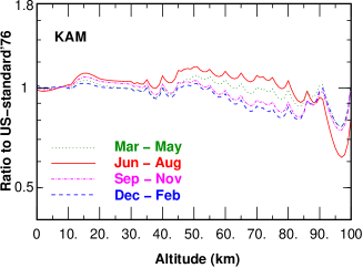
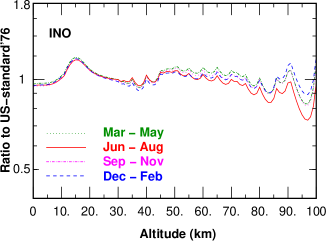
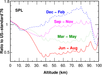
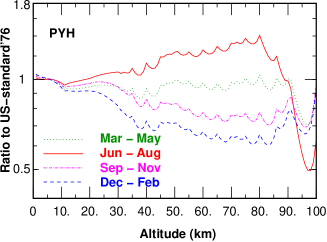
Figure 1: The ratio of air density in the NRLMSISE-00 atmospheric model to that of US-standard ’76 atmospheric model for the SK site (KAM), INO site (INO), South pole (SPL), and Pyhäsalmi mine (PYH), in the 4 seasons, March – May, June – August, September – November, and December – February.

In the tropical region (INO), we see a $\sim$ 20 % larger air density than the US-standard ’76 atmospheric model at the altitude of $\sim 15$ km a.s.l (above sea level). However, except for that, the air density profile is similar to the US-standard ’76 atmospheric model, and there is almost no seasonal variation by the NRLMSISE-00 atmospheric model. In the mid-latitude region (KAM), we find seasonal variations but they are small, and the air density profile is close to that of the US-standard ’76 atmospheric model through all the seasons below 40 km a.s.l. On the other hand, we find large seasonal variations in the Polar region (SPL and PYH) above 10 km a.s.l., especially at the South Pole (SPL). At the Pyhäsalmi mine, the air density profile is similar to that of the US-standard ’76 atmospheric model below 10 km a.s.l, but at the South Pole, the air density decreases quicker than that even below 10 km a.s.l.

Thus, we expect some seasonal variations of atmospheric neutrino flux except for the tropical region, and study it some in detail with the NRLMSISE-00 atmospheric model in the section V.

III Geomagnetic Field and Sites

We have already reported a large effect of geomagnetic field on the calculation of atmospheric neutrino flux for several sites in mid-latitude, such as SK and SNO sites Honda et al. (2004, 2011), through the rigidity cutoff and muon bending.

As a naive illustration of the rigidity cutoff, consider the gyro motion of cosmic rays guided by the horizontal component of the geomagnetic field near the Earth. The cosmic rays with a very small radius of gyro motion can not arrive at a very close point to the earth. As the radius of the gyro motion becomes larger, the cosmic rays can access the point, but the Earth works as a slant shield, limiting the access azimuth angle of cosmic rays. When the radius is large enough, the Earth becomes a flat shield just limiting the upward going cosmic rays, and the limitation on the access azimuth angle disappears. This mechanism is called the rigidity cutoff.

The effect of the muon bending on the atmospheric neutrino flux is often explained by the difference of the arrival zenith angle of neutrinos from that without the muon bending by the geomagnetic field. As the atmospheric neutrino flux above a few GeV has a large arrival zenith angle dependence, a little difference of the zenith angle results in a large difference of the flux separately visible from the rigidity cutoff at these energies. For the difference of the arrival zenith angle, the horizontal component of the geomagnetic field is responsible.

Thus, the horizontal component of geomagnetic field ($B_{h}$) is an important parameter to understand the effects of rigidity cutoff and muon bending. In Fig. 2, we draw the strength of the horizontal component of the geomagnetic field using the IGRF geomagnetic model for the year of 2010 with the position of the SK site ($B_{h}\sim 30000$nT), INO site ($B_{h}\sim 40000$nT), South Pole ($B_{h}\sim 16000$nT), and Pyhásalmi mine ($B_{h}\sim 13000$nT) for which we are going to calculate the atmospheric neutrino flux.

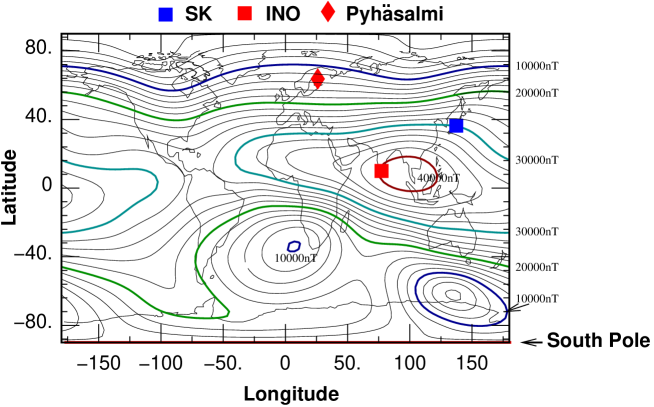
Figure 2: The horizontal component and the sites, Kamioka (KAM), South pole (SPL), INO site (INO), and Pyhäsalmi mine (PYH). where atmospheric neutrino flux is calculated.

IV Calculation of Atmospheric neutrino flux

Except for the atmospheric model, the calculation scheme, including the interaction model and the cosmic ray spectra model are the same as in the previous work Honda et al. (2011). We assume the surface of the Earth as a sphere with radius of $R_{e}=6378.140$ km. In addition, we assume 2 more spheres, the injection sphere with a radius of $R_{inj}=R_{e}+100$ km and escape sphere with radius $R_{esc}=10\times R_{e}$. Before Ref. Honda et al. (2007), we assumed one more, the simulation sphere with radius of $R_{sim}$ ($R_{inj}<R_{sim}<R_{esc}$). We discarded the cosmic rays which go outside of this sphere after the injection. We took $R_{sim}=R_{e}+3000$ km in Ref. Honda et al. (2007). However, now we identify the simulation sphere and the escape sphere by taking $R_{sim}=R_{esc}$ after Ref. Honda et al. (2011).

For each cosmic ray event simulation, we sample an energy and a chemical composition of cosmic ray to simulate, according to the cosmic ray spectra model. Then we sample the position and the initial direction of the cosmic ray on the injection sphere to start the simulation. For each cosmic ray, we apply the rigidity cutoff test and check if it reaches this position penetrating the rigidity cutoff.

This rigidity cutoff test is carried out by the back tracing method, solving the equation of motion in the inverse time direction in the geomagnetic field. When the sampled cosmic ray reaches the escape sphere without touching the injection sphere again, we judge that the cosmic ray can reach the starting position from deep space, and feed it into the simulator of the propagation in the atmosphere.

Generally, the transition from inhibited to allowed rigidity is not clear. Most cosmic rays, which fail the rigidity cutoff test, hit the injection sphere very quickly before completing one cycle of gyro motion. However, some of them with rigidity near the transition, travel a long distance before hitting the injection sphere. Also a cosmic ray with slightly higher rigidity than one which passes the rigidity cutoff test may fail the test even starting from the same position and direction.

A primary cosmic ray may pass through the injection sphere more than once. In this case we have to select the first entrance to avoid double counting. For this purpose, we require that the cosmic ray should not come back to the injection sphere again during back tracing.

The simulator of cosmic ray propagation in the atmosphere follows the motion of all the cosmic rays, both primary cosmic rays which passed the rigidity cutoff test and secondary cosmic rays produced in interactions of the cosmic rays recursively, until they reach the escape sphere, or hit the surface of the Earth, or interact with an air nucleus, or decay. Each neutrino produced in the cosmic ray interaction or decay is examined if its path will take it through the virtual detector assumed around the neutrino observation site, and when it goes through the virtual detector, it is registered and the number is used to calculate the atmospheric neutrino flux. We take a circle with radius of 1113.2 km as the virtual detector. Note, the radius corresponds a change in longitude of 10 degrees on the equator.

As the virtual detector is far larger than the real neutrino detector, we introduce the “virtual detector correction”. Assuming a circle with a radius of $\theta_{d}$ around the real detector as the virtual detector, the flux $\Phi_{d}$ defined as the average flux in the virtual detector may be written in the form as

$$\Phi_{d}=\Phi_{0}+\Phi_{0}^{(2)}\theta_{d}^{2}~{}+\dots,$$ (1)

with the flux $\Phi_{0}$ at the real detector Honda et al. (2007). Then, we can cancel out the $\Phi_{0}^{(2)}\theta_{d}^{2}$ term, using two fluxes $\Phi_{1}$ and $\Phi_{2}$ determined in the virtual detectors with radii $\theta_{1}$ and $\theta_{2}$ respectively as

$$\Phi_{0}\simeq\frac{\theta_{1}^{2}\Phi_{2}-\theta_{2}^{2}\Phi_{1}}{\theta_{1}^{2}-\theta_{2}^{2}}=\frac{\Phi_{2}-r^{2}\Phi_{1}}{1-r^{2}},$$ (2)

where $r=\theta_{2}$/$\theta_{1}$. We took $r=1/2$ in Ref. Honda et al. (2007), but optimize it to $r=1/\sqrt{2}$ in Ref. Honda et al. (2011) to minimize the statistical error.

V Atmospheric neutrino flux at each site

In Fig. 3, we show the one year average of atmospheric neutrino fluxes at the SK site, INO site, South Pole, and Pyhäsalmi mine, averaging over all the directions. The qualitative features are the same at all the sites. but we find a difference of flux among the sites by factor $\sim$ 3 at the low energy end due to the large difference of the cutoff rigidity among these sites. The differences of flux among the sites above 10 GeV is small in the figure. However we expect a large seasonal variations at South Pole and Pyhäsalmi mine, and we will study them in the next subsection some in detail.

V.1 Seasonal variation of the atmospheric neutrino flux

To study the seasonal variations, we calculate the ratio of seasonal fluxes to the yearly flux average, and show them in Fig. 4. Also the ratio of the flux calculated with the US-standard ’76 atmospheric model to the yearly flux average is shown in the panel for SK site below 1 TeV. Note, the calculation of the fluxes with the US-standard ’76 atmospheric model was carried out in the previous work Honda et al. (2011), and the statistics of the Monte Carlo simulation is poorer than that in the present work especially above 1 TeV.

At the mid-latitude region (SK site) and tropical region (INO site), the seasonal differences are small, and is difficult to see even in the ratio. On the other hand, the seasonal variaston is large in the Polar region, as the summer–winter difference reaches more than 10 % at the South Pole at 10 TeV, and more than 5 % at the Pyhäsalmi mine. At both sites, the atmospheric neutrino flux is higher in summer (December – February at the South Pole and June – August at the Pyhäsalmi mine). This may be understood by the fact that the air density at higher altitudes ($\gtrsim$ 15 km) is higher in the summer at both sites (see Fig. 1). We note the seasonal variation of the $\nu_{e}$ and $\bar{\nu}_{e}$ fluxes starts from $\lesssim$ 10 GeV, where that of the $\nu_{\mu}$ and $\bar{\nu}_{\mu}$ is still small.

The effect of the air density profile on the atmospheric neutrinos is generally discussed considering the relative probability of pions to decay or to interact with air nuclei. This effect works equally on all flavors of neutrino at high energies ($\gtrsim$ 100 GeV), where the probability of the parent pions to interact becomes comparable to that to decay, and may explain the large seasonal variation above 1 TeV. However, it does not explain the seasonal variation of the $\nu_{e}$ and $\bar{\nu}_{e}$ fluxes starting from $\lesssim$ 10 GeV, and the difference from that of the $\nu_{\mu}$ and $\bar{\nu}_{\mu}$ fluxes.

To explain these difference, we need to consider the muon propagation in the atmosphere. When the air shrinks down lower, the muons are created at lower altitudes, and the probability of muons to hit the ground before decaying increases. When the muons hit the rock or ice, they lose their energy quickly producing neutrinos with very low energies ($\lesssim$ 0.1 GeV) only. Then the flux of neutrinos produced in the decay of muons decreases. This mechanism results in the variation of neutrino flux near the vertical directions at relatively high energies ($\gtrsim$ 10 GeV). It explain the variation of neutrino flux there, and the difference of the $\nu_{e}$ and $\bar{\nu}_{e}$ fluxes and the $\nu_{\mu}$ and $\bar{\nu}_{\mu}$ fluxes, as half of the $\nu_{\mu}$ and $\bar{\nu}_{\mu}$ are created in the pion decay directly.

There is another mechanism which has a large effect on the energy spectra of neutrinos at lower energies. When the atmosphere shrinks lower, the muons travel in denser air and lose more energy before the decay. The larger energy loss of the muons causes a shift to the energy spectra of the neutrinos produced in the muon decay towards the lower energy direction. As the energy spectra of atmospheric neutrinos are steeply decreasing at the energies $\gtrsim$ 0.1 GeV, the fluxes decrease in the denser air at those energies. However, this mechanism is effective when most muons decay in the air ($E_{\mu}\lesssim$ GeV), and for the neutrinos with energies below a few GeV. This mechanism is responsible to the seasonal variation of neutrino flux below 10 GeV.

The differences between the fluxes calculated with the US-standard ’76 atmospheric model and yearly averaged one at the SK site are far less than 5 %. It is difficult to say that the differences are due to the difference in the atmospheric model, since there are some improvement in the calculation scheme and statistics of Monte Carlo simulation after the previous work Honda et al. (2011).

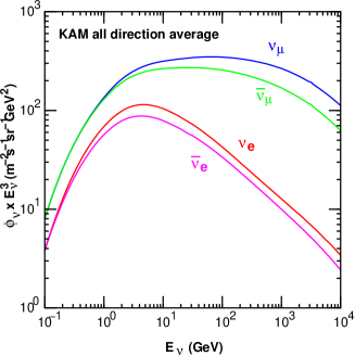
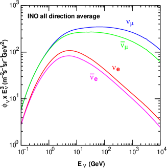
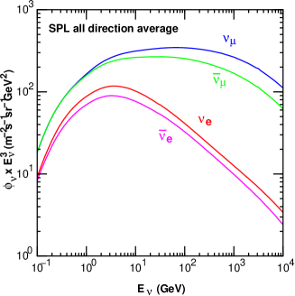
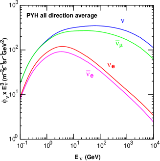
Figure 3: All-direction averaged atmospheric neutrino flux for 4 sites averaging over one year. KAM stands for the SK site, INO for the INO site, SPL for the South Pole, and PYH for the Pyhäsalmi mine.

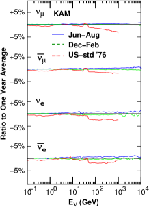
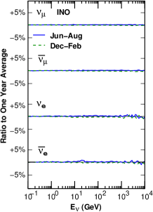
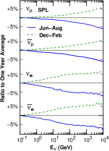
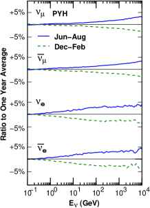
Figure 4: Ratios of the all-direction averaged flux in June – August and in December – February to that of the yearly average. For the SK site, we also plot the ratio for the calculation with the US-standard ’76 atmospheric model to the yearly average in dash-dot below 1 TeV.

V.2 Flavor-ratio of the atmospheric neutrino flux

In Fig. 5, we show the flavor-ratio defined as the flux ratio of different neutrino flavors such as, $(\nu_{\mu}+\bar{\nu}_{\mu})/(\nu_{e}+\bar{\nu}_{e})$, $(\nu_{\mu}/\bar{\nu}_{\mu})$, and $(\nu_{e}/\bar{\nu}_{e})$ at the SK site, INO site, South Pole, and Pyhäsalmi mine, averaging over all the directions. We find that the flavor-ratio is very similar to each other among these sites, confirming the stability of the flavor-ratio. However, the flavor-ratio is an important quantity in the study of neutrino oscillations, so we need to study the seasonal variations and position dependence’s more precisely.

To see the seasonal variation of the flavor-ratio, we calculate the ratio of the flavor-ratio calculated with the seasonally averaged fluxes to that calculated with the yearly averaged fluxes and plot them in Fig. 6 for each site. Also, to see the positional dependence on the earth, we take the flavor-ratio calculated with the yearly averaged fluxes at the SK site as the “reference flavor-ratio”. Then we calculate the ratio of the “reference flavor-ratio” to those calculated with yearly averaged fluxes at other sites, and plotted them in their panels of Fig. 6. While in the panel of the SK site, we show the ratio of the flavor-ratio calculated with the US-standard ’76 atmospheric model to that calculated with the yearly averaged fluxes at the SK site (i.e. the “reference flavor-ratio”).

At the sites in the Polar region (South Pole and Pyhäsalmi mine), the flavor-ratio, $(\nu_{\mu}+\bar{\nu}_{\mu})/(\nu_{e}+\bar{\nu}_{e})$ shows a seasonal variation, high in summer and low in winter, with the maximum of the amplitude at $\sim$ 100 GeV. This is considered to be due to the seasonal variation of the altitude of cosmic ray interactions. Also the flavor-ratio shows some differences from the SK site at the energy below a few GeV. This is considered to be due to the lower air density at the neutrino production height of 10$\sim$20 km a.s.l (see section VI) in the Polar region. The smaller muon energy loss causes a smaller shifts of the energy spectra of the neutrinos produced in the muon decay .

Note, the air density at the South pole at the 10$\sim$20 km a.s.l. is much lower than at the Pyhäsalmi mine in Fig. 1, but the difference of the flavor-ratio, $(\nu_{\mu}+\bar{\nu}_{\mu})/(\nu_{e}+\bar{\nu}_{e})$ at the South Pole from the SK site is similar to that at the Pyhäsalmi mine. This is considered to be due to the higher observation site at the South Pole (2835m a.s.l.). The shorter distance from the ground to the production height of muons reduces the neutrino fluxes produced by muon decay at the South Pole.

In the $\nu_{e}/\bar{\nu}_{e}$ ratio, we also find a difference from the SK site at the South Pole and Pyhäsalmi mine, below a few GeV. This difference is considered to be due to the difference of cutoff rigidity. The $\nu_{e}/\bar{\nu}_{e}$ ratio reflects the $\pi^{+}/\pi^{-}$ ratio of parent pions. As the majority of primary cosmic rays are protons, there is a $\pi^{+}$ excess generally. Especially when the cutoff rigidity is low enough, the pion production of primary cosmic rays overwhelms that of secondary cosmic rays, and $\pi^{+}/\pi^{-}$ and $\nu_{e}/\bar{\nu}_{e}$ ratios are high even at low energies. However, when cutoff rigidity is high, the pion production by secondary cosmic rays can not be ignored, and the $\pi^{+}$ excess is diluted by the secondary neutron cosmic ray interactions.

In the comparison of neutrino flavor-ratio between the SK site (mid-latitude region) and the INO site (tropical region), we find a small difference in the $(\nu_{\mu}+\bar{\nu}_{\mu})/(\nu_{e}+\bar{\nu}_{e})$ ratio due to the difference of air density at $15$ km a.s.l., and the difference of the muon energy loss. Other ratios are quite similar to each other. The differences of the flavor-ratio with the US-standard ’76 atmosphere model are very small to that in the present calculation.

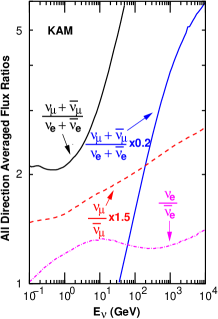
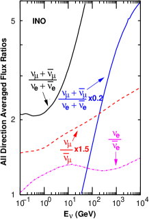
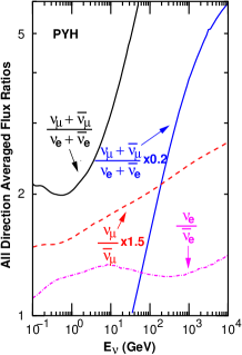
Figure 5: Neutrino flavor-ratio calculated with the all-direction and one-year averaged atmospheric neutrino flux. KAM stands for the SK site, INO for the INO site, SPL for the South Pole, and PYH for the Pyhäsalmi mine.

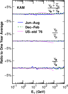
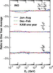
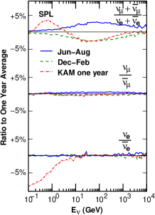
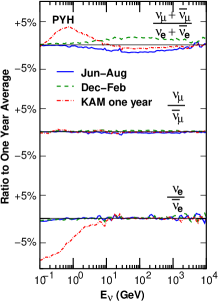
Figure 6: Ratios of the flavor-ratio calculated with the all-direction and seasonally averaged flux to that calculated with all-direction and yealy averaged flux. The solid lines are the flux ratio in June – August, and dashed lines are in December – February. KAM stands for the SK site, INO for the INO site, SPL for the South Pole, and PYH for the Pyhäsalmi mine. Taking the yealy averaged flavor-ratio at SK-site as the ’‘reference flavor-ratio”, the ratio of ’‘reference flavor-ratio” to the yearly averaged flavor-ratio at each site are plotted with dash-dot other than the panel for the SK-site. In the panel for the SK-site, the ratio of the flavor-ratio with the US-standard ’76 atmospheric model to the yearly averaged flavor-ratio at SK-site is plotted with dash-dot.

V.3 Zenith angle variation of the atmospheric neutrino flux at 3.2 GeV

In Fig. 7, we show the the zenith angle dependence of the atmospheric neutrino flux calculated at the 4 sites at 3.2 GeV. We also plot the atmospheric neutrino flux calculated with the US-standard ’76 atmospheric model Honda et al. (2011) at the SK site, although the differences are small and within the thickness of the line. The seasonal variation is very small at the SK and INO sites as in the all-direction average, but is seen clearly in the down going neutrino fluxes at the South Pole and Pyhäsalmi mine even at this energy. At both the sites the trend is the same as the all-direction average at high energies, the atmospheric neutrino flux is large in summer (June – August at Pyhäsalmi mine and December – February at the South Pole).

The amplitude of the seasonal variation is different among different neutrino flavors in Fig. 7. It is $\sim$ 2.5% for $\nu_{\mu}$ and $\bar{\nu}_{\mu}$, and $\sim$ 10 % for $\nu_{e}$ and $\bar{\nu}_{e}$ for the vertically down going direction at the South Pole. The muon energy loss in the atmosphere before the decay seems to be mainly responsible to this seasonal variations.

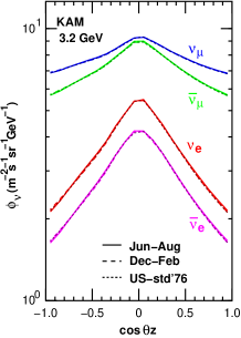
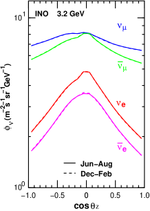
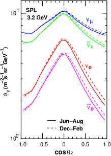
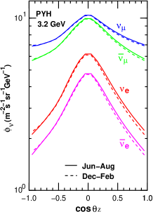
Figure 7: Arrival zenith angle dependence of atmospheric neutrino fluxes averaged over all azimuth angles at 3.2 GeV. KAM stands for the SK site, INO for the INO site, SPL for the South Pole, and PYH for the Pyhäsalmi mine. The solid lines are the time average in June – August, and dashed lines are in December – February. For SK site, we also plot the calculation with the US-standard ’76 atmospheric model using a dotted line (but is difficult to see separately). Note, $\theta_{z}$ stands for the zenith angle.

Leaving from the seasonal variation, the atmospheric neutrino flux at near horizontal directions are largely different from site to site. The horizontal fluxes at the SK site are $\sim 10$ % smaller than those at the South Pole or Pyhäsalmi mine, but $\sim 10$ % larger than those at the INO site. The differences in the atmospheric neutrino fluxes at near horizontal directions is mainly caused by the difference of rigidity cutoff at near horizontal directions. The rigidity cutoff works most strongly for the neutrinos arriving from near horizontal geomagnetic East directions. At the SK site, we can almost ignore the rigidity cutoff at near vertical directions, but it is still strong at near horizontal directions. We can explain the difference between the SK site and the Polar region by the difference of rigidity cutoff, but can not explain the difference between INO and SK sites only by the difference of rigidity cutoff. We need to consider the muon bending, as the suppression for the $\nu_{\mu}$ and $\bar{\nu}_{e}$ is stronger than that for $\bar{\nu}_{\mu}$ and $\nu_{e}$ at the INO site. The suppression by the muon bending will be understood better with the azimuthal variation of atmospheric neutrinos described in subsection V.4.

The fluxes at the South Pole and Pyhäsalmi mine are a little smaller than the SK and INO sites at $\cos\theta_{z}\sim-0.7$, and they have some structure there due to the rigidity cutoff and the muon bending at the places where the neutrinos are produced. On the other hand, the rigidity cutoff and the muon bending effects are weaker at the SK and INO sites at $\cos\theta_{z}\sim-0.7$ than the South Pole and Pyhäsalmi mine.

Apart from the geomagnetic field, the vertically down going neutrino fluxes at the South Pole are a little smaller than those at the Pyhäsalmi mine due to the difference of the observation altitudes. For the South Pole, 2835m a.s.l. is assumed as the observation site, and sea level for Pyhäsalmi mine.

V.4 Azimuthal variation of atmospheric neutrino flux

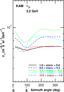
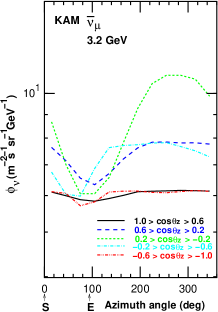
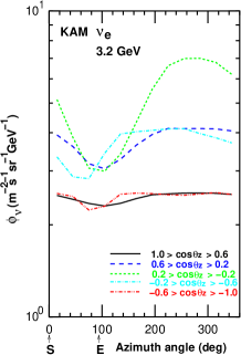
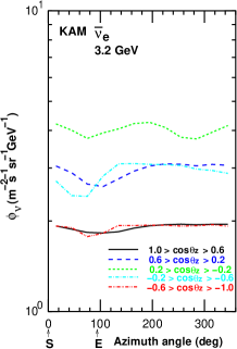
Figure 8: Arrival azimuth angle dependence of the time averaged atmospheric neutrino flux in 5 zenith angle bins, $1>\cos\theta_{z}>0.6$, $0.4>\cos\theta_{z}>0.2$, $0.2>\cos\theta_{z}>-0.2$, $-0.2>\cos\theta_{z}>-0.6$, and $-0.6>\cos\theta_{z}>-1$ at the SK site. The azimuth angle is measured counter-clockwise from South. Solid line shows the averaged fluxe in $1>\cos\theta_{z}>0.6$, dashed line that in $0.4>\cos\theta_{z}>0.2$, dotted line that in $0.2>\cos\theta_{z}>-0.2$, dash dot that in $-0.2>\cos\theta_{z}>-0.6$, and dash 2dots aht in $-0.6>\cos\theta_{z}>-1$.

Next, we study the azimuthal variation of the neutrino fluxes in 5 zenith angle bins; $1>\cos\theta_{z}>0.6$, $0.4>\cos\theta_{z}>0.2$, $0.2>\cos\theta_{z}>-0.2$, $-0.2>\cos\theta_{z}>-0.6$, and $-0.6>\cos\theta_{z}>-1$ at 3.2 GeV, averaging over a year. In Fig. 8, we show the azimuthal variation of atmospheric neutrino flux at the SK site, in Fig. 9, those at the INO site, in Fig. 10, those at the South Pole and in Fig. 11, those at the Pyhäsalmi mine.

In these figures we observe two kinds of effects from the geomagnetic field. One is the rigidity cutoff, and the other is the muon bending. The geomagnetic field directed to the North filters the low energy cosmic rays from the East directions, since the cosmic rays generally carry a positive charge. The rigidity cutoff reduces all flavors of neutrino from the East at the same rate.

On the other hand, the effect of muon bending depends on the muon charge. The positive muon and its decay products are affected by the geomagnetic field in the same way as the rigidity cutoff, and the negative muon and its decay products are affected in the opposite way. Then, muon bending reduces the $\bar{\nu}_{\mu}$ and $\nu_{e}$ fluxes from the East, but reduces the $\nu_{\mu}$ and $\bar{\nu}_{e}$ fluxes from the West.

In Fig. 8, we find small azimuthal variations of atmospheric neutrino fluxes at near vertically down going directions ($1>\cos\theta_{z}>0.6$) at the SK site. As the variation shape is almost the same among all neutrino flavors, this variation is considered to be due to the rigidity cutoff, but the effect is already small at the SK site for near vertical directions at 3.2 GeV.

At near horizontal directions ($0.2>\cos\theta_{z}>-0.2$), $\bar{\nu}_{\mu}$ and $\nu_{e}$ fluxes have large sinusoidal azimuthal variations, but $\nu_{\mu}$ and $\bar{\nu}_{e}$ fluxes have small but more complicated azimuthal variations. This is because the rigidity cutoff and the muon bending work in the same directions for $\bar{\nu}_{\mu}$ and $\nu_{e}$ fluxes, and in the opposite directions for $\nu_{\mu}$ and $\bar{\nu}_{e}$ fluxes. The dip at $\sim 90^{\circ}$ commonly seen in all neutrino flavors is considered to be due to the rigidity cutoff, and the dip at $\sim 270^{\circ}$ seen in the $\nu_{\mu}$ and $\bar{\nu}_{e}$ fluxes is due to muon bending.

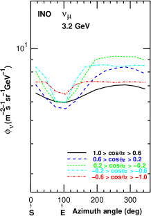
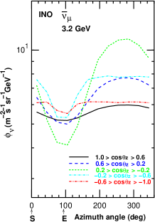
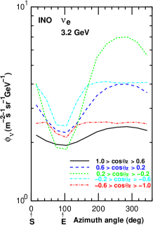
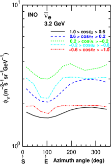
Figure 9: Azimuth angle dependence of the time averaged atmospheric neutrino flux in 5 zenith angle bins, $1>\cos\theta_{z}>0.6$, $0.4>\cos\theta_{z}>0.2$, $0.2>\cos\theta_{z}>-0.2$, $-0.2>\cos\theta_{z}>-0.6$, and $-0.6>\cos\theta_{z}>-1$ at the INO site. The azimuth angle is measured counter-clockwise from the South. Solid line shows the averaged fluxe in $1>\cos\theta_{z}>0.6$, dashed line that in $0.4>\cos\theta_{z}>0.2$, dotted line that in $0.2>\cos\theta_{z}>-0.2$, dash dot that in $-0.2>\cos\theta_{z}>-0.6$, and dash 2dots aht in $-0.6>\cos\theta_{z}>-1$.

In Fig. 9, we find larger azimuthal variations of atmospheric neutrino fluxes at near vertically down going directions ($1>\cos\theta_{z}>0.6$) at the INO site compared to the SK site. As the variation shape is similar among all neutrino flavors, this is considered as an effect of the rigidity cutoff, and is still strong at the INO site for vertical down going directions at 3.2 GeV. The azimuthal variation at near horizontal directions ($0.2>\cos\theta_{z}>-0.2$) are also larger than the SK site for each neutrino flavor, due to the larger horizontal component of the geomagnetic field.

We note that the muon bending effect is seen in the azimuthal averaged flux plot (Fig. 7) at the INO site at near horizontal directions. The muon bending suppresses the $\nu_{\mu}$ and $\bar{\nu}_{e}$ fluxes from the West, but enhances them from the East. However, the rigidity cutoff works strongly for the East directions, canceling the enhancement from the East, and the muon bending is seen as a suppression of the $\nu_{\mu}$ and $\bar{\nu}_{e}$ fluxes in Fig. 7. On the other hand for $\bar{\nu}_{\mu}$ and $\nu_{e}$, the muon bending enhances the fluxes from the West, but suppresses them from the East. As the rigidity cutoff works weakly for the West directions, the muon bending is seen as an enhancement of the $\bar{\nu}_{\mu}$ and $\nu_{e}$ fluxes in Fig. 7. The same mechanism works at other sites, but the amplitudes of the suppression and enhancement are small, and it is not seen clearly even at the SK site (KAM).

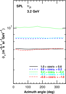
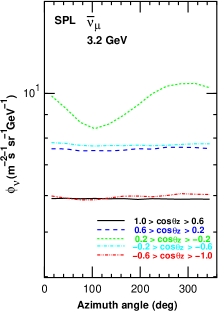
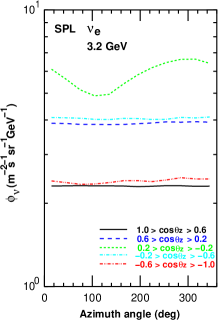
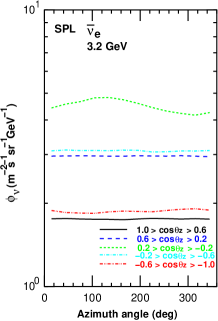
Figure 10: Azimuth angle dependence of the time averaged atmospheric neutrino flux in 5 zenith angle bins, $1>\cos\theta_{z}>0.6$, $0.4>\cos\theta_{z}>0.2$, $0.2>\cos\theta_{z}>-0.2$, $-0.2>\cos\theta_{z}>-0.6$, and $-0.6>\cos\theta_{z}>-1$ at the South Pole. The azimuth angle is measured counter-clockwise from the meridian line of 180 degree in longitude. Solid line shows the averaged fluxe in $1>\cos\theta_{z}>0.6$, dashed line that in $0.4>\cos\theta_{z}>0.2$, dotted line that in $0.2>\cos\theta_{z}>-0.2$, dash dot that in $-0.2>\cos\theta_{z}>-0.6$, and dash 2dots aht in $-0.6>\cos\theta_{z}>-1$.

In Fig. 10, we find that there are almost no azimuthal variations of the atmospheric neutrino flux except for the near horizontal directions ($0.2>\cos\theta_{z}>-0.2$) at the South Pole, since the geomagnetic field is almost vertical at the South Pole. At near horizontal directions we find the azimuthal variations of the $\bar{\nu}_{\mu}$ and $\nu_{e}$, having the minimum at $\sim$ 90^∘ and the maximum at $\sim$ 270^∘. Also there are slightly smaller variations of $\nu_{\mu}$ and $\bar{\nu}_{e}$, having the minimum at $\sim$ 90^∘ and the maximum at $\sim$ 270^∘. These features represent the fact that the rigidity cutoff works very weakly at the South Pole, and the muon bending works mainly with the residual horizontal component of the geomagnetic field. We note that the azimuthal variation for upward going directions ($\cos\theta_{z}<-0.2$) is also very small at the South pole. This is probably because the South Pole is close to the geomagnetic South pole in the dipole approximation of the geomagnetic field.

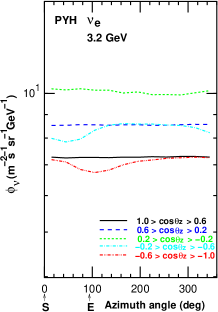
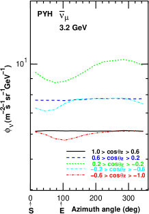
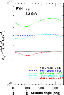
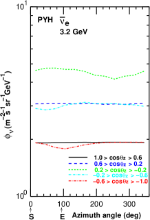
Figure 11: Azimuth angle dependence of the time averaged atmospheric neutrino flux in 5 zenith angle bins, $1>\cos\theta_{z}>0.6$, $0.4>\cos\theta_{z}>0.2$, $0.2>\cos\theta_{z}>-0.2$, $-0.2>\cos\theta_{z}>-0.6$, and $-0.6>\cos\theta_{z}>-1$ at the Pyhäsalmi mine. The azimuth angle is measured counter-clockwise from the South. Solid line shows the averaged fluxe in $1>\cos\theta_{z}>0.6$, dashed line that in $0.4>\cos\theta_{z}>0.2$, dotted line that in $0.2>\cos\theta_{z}>-0.2$, dash dot that in $-0.2>\cos\theta_{z}>-0.6$, and dash 2dots aht in $-0.6>\cos\theta_{z}>-1$.

In Fig. 11, we find the features of azimuthal variations of down going and near horizontal atmospheric neutrino flux ($\cos\theta_{z}>-0.2$) at the Pyhäsalmi mine are almost the same as those at the South Pole. We note that the horizontal component of the geomagnetic field at the Pyhäsalmi mine ($B_{h}\sim 13000$ nT) is even smaller than that of the South Pole ($B_{h}\sim 16000$ nT). However, as the Pyhäsalmi mine sits at a distant position from the geomagnetic North Pole, the rigidity cutoff and muon bending affects the azimuthal variations of the upward going neutrinos.

VI production height of atmospheric neutrino

Here we study the production heights of atmospheric neutrinos calculated with the NRLMSISE-00 atmospheric model. The production height is an important parameter for analyzing the neutrino oscillations using atmospheric neutrinos. As the production heights are distributed in a wide range from sea level to $\sim$ 100 km a.s.l., we examine the cumulative distribution, and plot the height where the cumulative distribution of production height reaches 10 %, 50 %, and 90 % as a function of neutrino energy for vertical down going neutrinos ($\cos\theta_{z}>0.9$) and horizontally going neutrinos ($0.1>\cos\theta_{z}>0$) in Figs 12, 13, 15, and  14, In those figures, the heights shown by the lines of 10 %, 50 %, and 90 % indicate 10 %, 50 %, and 90 % of neutrinos are created below those height, respectively. for the SK site, INO site, South Pole, and Pyhäsalmi mine respectively. To make the distributions in the figures, we combine particle and anti-particle neutrinos, and average over all azimuth angles. In the figures for the SK site, we also plot the same flavor-ratio with the US-standard ’76 atmospheric model below 32 GeV, calculated in the previous work Honda et al. (2011).

The production heights are largely different between $\nu_{\mu}$ + $\bar{\nu}_{\mu}$ and $\nu_{e}$ + $\bar{\nu}_{e}$, and also between vertical and horizontal directions. The large energy dependence of production height of the $\nu_{e}$ and $\bar{\nu}_{e}$ are explained by the fact that they are mainly produced by muon decay in the energies $\lesssim$ 100 GeV for near vertical directions, and $\lesssim$ 1 TeV for near horizontal directions. The muons fly long distances before decays, and make neutrinos at a lower altitude. As the muon flight length increases with the muon energy, the production height of the $\nu_{e}$ and $\bar{\nu}_{e}$ becomes lower as long as the muon is their major source. However, above 100 GeV for vertical directions and 1 TeV for horizontal directions, Kaon decay becomes the main source, then the production height becomes high again.

Muon decay is also a source of $\nu_{\mu}$ and $\bar{\nu}_{\mu}$. A similar variation to $\nu_{e}$ and $\bar{\nu}_{e}$ is also seen in $\nu_{\mu}$ and $\bar{\nu}_{\mu}$, but with a smaller amplitude. The fraction of $\nu_{\mu}$ and $\bar{\nu}_{\mu}$ created in muon decay is not so large, roughly a half at low energies and decreasing with the energy as muons tend to hit the ground. The effect of muon flight in the production height is smaller on $\nu_{\mu}$ and $\bar{\nu}_{\mu}$ than that on $\nu_{e}$ and $\bar{\nu}_{e}$.

Note, above 100 GeV for vertical directions and 1 TeV for horizontal directions, Kaon decay becomes the main source of all flavors of neutrinos. Then the production height becomes high, close to the production height of Kaons, or the hadronic interaction zone of cosmic rays. We would also like to note that the production height calculated in 3D-scheme is smoothly connected to that calculated in the 1D-scheme as well as the flux.

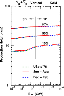
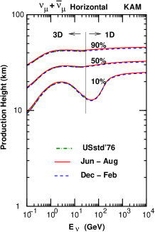
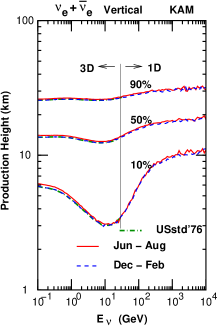
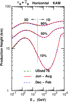
Figure 12: Production height of atmospheric neutrinos for $\nu_{\mu}$ + $\bar{\nu}_{\mu}$ and $\nu_{e}$ + $\bar{\nu}_{e}$ going to vertically down and horizontal directions, summing all azimuth directions at the SK site. The height that cumulative distribution reaches 10 %, 50 %, and 90 % are shown as the function of neutrino energy. The time average values in June – August are shown as solid lines and in December – February as Dashed line. The same values with the US-standard ’76 atmospheric model are also shown in dash dot in the 3D region.

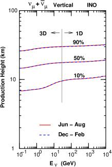
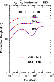
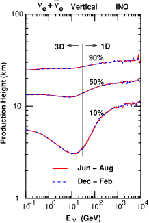
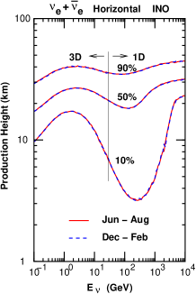
Figure 13: Production height of atmospheric neutrinos for $\nu_{\mu}$ + $\bar{\nu}_{\mu}$ and $\nu_{e}$ + $\bar{\nu}_{e}$ going to vertical down and horizontal directions, summing all azimuth directions at the INO site. The height that cumulative distribution reaches 10 %, 50 %, and 90 % are shown as a function of neutrino energy. The time average values in June – August are shown as solid lines and in December – February as Dashed line.

At the SK and INO sites, we observe small difference between the averages of June – August and December – February. Especially at the INO site, the difference is almost invisible in the figures. The difference between the calculations with the NRLMSISE-00 and US-standard ’76 atmospheric models at the SK site is also small. On the other hand, we find a large seasonal variation of production height at the South Pole. The variation of the median (cumulative distribution of 50 %) height extend to $\sim$ 20% variation at near horizontal directions, and the variation of the amplitude is similar between $\nu_{\mu}$ + $\bar{\nu}_{\mu}$ and $\nu_{e}$ + $\bar{\nu}_{e}$. At the Pyhäsalmi mine, we also find a seasonal variation of $\sim$ 10 % for the median.

The energy dependence of the production height is similar among the different sites. However, the of 10 % line of the cumulative distribution for $\nu_{e}$ + $\bar{\nu}_{e}$ at the South Pole is a little higher than that at other sites due to the altitude of the sites, as we assumed the observation site is 2835m a.s.l. for the South Pole, and sea level for other sites.

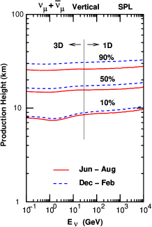
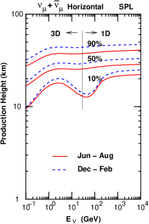
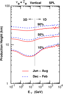
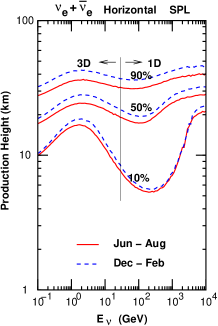
Figure 14: Production height of atmospheric neutrinos for $\nu_{\mu}$ + $\bar{\nu}_{\mu}$ and $\nu_{e}$ + $\bar{\nu}_{e}$ going to vertically down and horizontal directions, summing all azimuth directions at the South Pole. The height that cumulative distribution reaches 10 %, 50 %, and 90 % are shown as a function of neutrino energy. The time average values in June – August are shown as solid lines and in December – February as Dashed line.

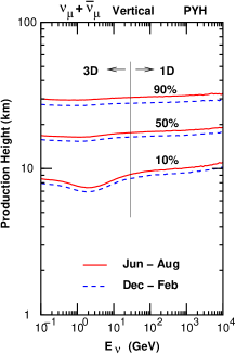
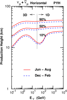
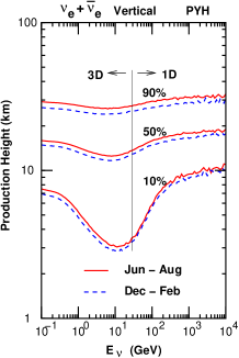
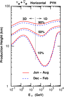
Figure 15: Production height of atmospheric neutrinos for $\nu_{\mu}$ + $\bar{\nu}_{\mu}$ and $\nu_{e}$ + $\bar{\nu}_{e}$ going to vertically down and horizontal directions, summing all azimuth directions at the Pyhäsalmi mine. The height that cumulative distribution reaches 10 %, 50 %, and 90 % are shown as a function of neutrino energy. The time average values in June – August are shown as solid lines and in December – February as Dashed line.

In Fig. 16 we plotted the azimuthal variation of the median of the production height at near horizontal directions for the atmospheric neutrinos at $E_{\nu}=3.36$ GeV ($3.16<E_{\nu}<3.55$ GeV), summing the production height distribution over a year. We find there are sinusoidal variations with azimuth angle for all flavor neutrinos, but in an opposite direction to each other among the neutrinos and anti-neutrinos, at the SK and INO site. The azimuth variation of production height at the Pyhäsalmi mine is smaller than that at the SK and INO sites, but the shape is similar. The azimuthal variation of production height at the South Pole is small. These sinusoidal features at the SK and INO sites could be understood if we consider that the production height is mainly controlled by the horizontal component of the geomagnetic field and the effect of the rigidity cutoff is small.

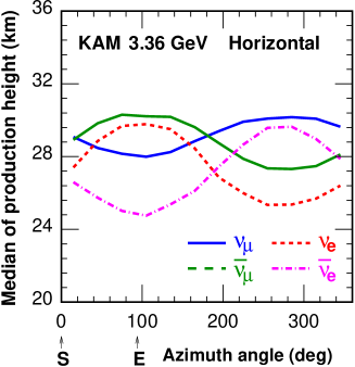
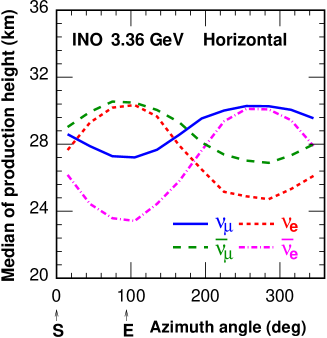
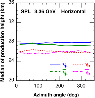
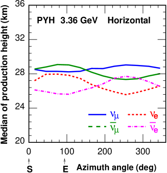
Figure 16: Azimuthal variation of production height of atmospheric neutrinos at the SK site, INO site, South Pole and Pyhäsalmi mine for near horizontal directions. The height that cumulative distribution reaches 50 % is shown as the function of azimuth for neutrino in the energy range of $3.16<E_{\nu}<3.55$ GeV.

VII summary and discussion

We have extended our calculation of atmospheric neutrino flux to the tropical (INO site) and polar regions (South Pole and Pyhäsalmi mine). In this extension, we have updated the atmospheric model from the US-standard ’76 model to the NRLMSISE-00 model. When we compare the two atmospheric models, we find the NRLMSISE-00 atmospheric model almost agrees with the US-standard ’76 atmospheric model in the tropical and mid-latitude region. However, they disagree with each other largely in the polar region. Also the NRLMSISE-00 atmospheric model suggests a large seasonal variation in the polar region. The atmospheric neutrino flux calculated with the NRLMSISE-00 model is compared with that calculated with the US-standard ’76 model at the SK site.

Adding to the air density profile, there is a large difference of the geomagnetic field configuration between equatorial and polar regions. It is well known that the influence of geomagnetic field on the atmospheric neutrino is large. The extension in this paper is also the study of the atmospheric neutrino flux in the two extremes in the IGRF geomagnetic field model. Note, our calculation so far was limited to the sites in mid-latitude region.

As expected, the calculated atmospheric neutrino flux at the equatorial (tropical) site (INO) suffers a strong effect from the horizontal component of the geomagnetic field. A large reduction of the neutrino flux is still seen at 3.2 GeV for down going directions due to the rigidity cutoff. The muon bending causes a large azimuthal variation of neutrino fluxes. reducing $\nu_{\mu}$ and $\bar{\nu}_{e}$ fluxes and enhancing a little $\bar{\nu}_{\mu}$ and $\nu_{e}$ flues at horizontal directions.

On the other hand, the large seasonal variation of air density profile at the polar regions (South Pole and Pyhäsalmi mine) causes a large seasonal variation of atmospheric neutrino flux. We had expected that the seasonal dependence is large at higher energies since the $\pi$ decay and interaction ratio changes with the air density. But at the South Pole, a $\sim$ 10 % variation is seen even at 3.2 GeV in the $\nu_{e}$ and $\bar{\nu}_{e}$ fluxes for vertically down going directions. The fluxes of the $\nu_{\mu}$ and $\bar{\nu}_{\mu}$ also show variations, but smaller than those of the $\nu_{e}$ and $\bar{\nu}_{e}$. This is considered to be due to the change of muon energy loss rate in the atmosphere according to the change of the air density by the seasons.

We also studied the production height of atmospheric neutrinos with the NRLMSISE-00 atmospheric model. For the mid-latitude region (SK site), they are very close to the production height calculated with the US-standard ’76 atmospheric model. In the polar region, we find a seasonal variation of production height, but in the mid-latitude and tropical regions, the seasonal variation of production height is small, and almost invisible. However, we find a large azimuthal variation of production height due to the muon bending in the mid-latitude and tropical regions.

Here, we would like to make a short comment on the calculation error of the atmospheric neutrino flux, and on the recent observations of the cosmic rays. First note that this work is still within the calculation scheme established in Ref Honda et al. (2007) which is based on the comparison of atmospheric muon observation and calculation. Therefore, the estimation made in Ref Honda et al. (2007) is still valid in this work. The total error is a little lower than 10 % in the energy region 1–10 GeV. The error increases outside of this energy region due to the small number of available muon observation data at the lower energies, and due to the uncertainty of Kaon production at higher energies.

The recent observations of the primary cosmic rays Wefel et al. (2005); Yoon et al. (2011); Adriani et al. (2011); Aguilar et al. (2015), suggest that we need to modify the interaction model again to reconstruct the observed atmospheric muon fluxes with them. In a preliminary work Honda (2011), we find it is possible to modify the interaction model in such a way. and the atmospheric neutrino flux calculated with that is very close to the present calculation in 1–10 GeV and well within the error estimated in Ref Honda et al. (2007). Now would be the time to study the interaction model with the updated primary cosmic ray spectra model for the calculation of atmospheric neutrino flux.