Baseband Modulation Instability as the Origin of Rogue Waves

Abstract

We study the existence and properties of rogue wave solutions in different nonlinear wave evolution models that are commonly used in optics and hydrodynamics. In particular, we consider Fokas-Lenells equation, the defocusing vector nolinear Schrödinger equation, and the long-wave-short-wave resonance equation. We show that rogue wave solutions in all of these models exist in the subset of parameters where modulation instability is present, if and only if the unstable sideband spectrum also contains cw or zero-frequency perturbations as a limiting case (baseband instability). We numerically confirm that rogue waves may only be excited from a weakly perturbed cw whenever the baseband instability is present. Conversely, modulation instability leads to nonlinear periodic oscillations.

I Introduction

Many nonlinear wave equations associated with different physical systems exhibit the emergence of extreme, high-amplitude events that occur with low probability, and yet may have dramatic consequences.

Perhaps the most widely known examples of such processes are the giant oceanic rogue waves hopkin04 that unexpectedly grow with a great destructive power from the average sea level fluctuations. This makes the study of rogue waves a very important problem for ocean liners and hydrotechnic constructions perkin06 ; pelinosky08 . Hence, it is not surprising that the phenomenon of rogue waves has attracted the ample attention of oceanographers over the last decade. Although the existence of rogue waves has been confirmed by multiple observations, uncertainty still remains on their fundamental origins kharif09 .

In recent years, research on oceanic rogue waves has also drawn the interest of researchers in many other domains of physics and enginering applications, which share similar complexity features: in particular, consider nonlinear optics dud14 . The ongoing debate on the origin and definition of rogue waves has stimulated the comparison of their predictions and observations in hydrodynamics and optics, since analogous dynamics can be identified on the basis of their common mathematical models onorato13 .

So far, the focusing nonlinear Schrödinger equation (NLSE) has played a pivotal role as universal model for rogue wave solutions, boh in optics and in hydrodynamics. For example, the Peregrine soliton, first predicted as far as $30$ years ago peregrine83 , is the simplest rogue-wave solution of the focusing NLSE. This rogue wave has only recently been experimentally observed in optical fibers kibler10 , water-wave tanks amin11 , and plasmas bailung11 .

For several systems the standard focusing NLSE turns out to be an oversimplified description: this fact pushes the research to move beyond this model. In this direction, recent developments consist in including the effect of dissipative terms. In fact, a substantial supply of energy (f.i., from the wind in oceanography, or from a pumping source in laser cavities) is generally required to drive rogue wave formation lecap12 . Because of their high amplitude or great steepness, rogue wave generation may be strongly affected by higher-order perturbations, such as those described by the Hirota equation ankiew10 , the Sasa-Satsuma equation bandel12 and the derivative NLSE chen14 .

The study of rogue wave solutions to coupled wave systems is another hot topic, where several advances were recently reported. Indeed, numerous physical phenomena require modeling waves with two or more components. When compared to scalar dynamical systems, vector systems may allow for energy transfer between their different degrees of freedom, which potentially yields rich and significant new families of vector rogue-wave solutions. Rogue-wave families have been recently found as solutions of the vector NLSE (VNLSE)baronio12 ; liu2013 ; zhai2013 ; baronio14 , the three-wave resonant interaction equations baronio13 , the coupled Hirota equations chen13 , and the long-wave-short-wave resonance chen14R .

As far as rogue waves excitation is concerned, it is generally recognized that modulation instability (MI) is among the several mechanisms which may lead to rogue wave excitation. MI is a fundamental property of many nonlinear dispersive systems, that is associated with the growth of periodic perturbations on an unstable continuous-wave background zakh09 . In the initial evolution of MI, sidebands within the instability spectrum experience an exponential amplification at the expense of the pump. The subsequent wave dynamics is more complex and it involves a cyclic energy exchange between multiple spectral modes. In fiber optics, MI seeded from noise results in a series of high-contrast peaks of random intensity. These localized peaks have been compared with similar structures that are also seen in studies of ocean rogue waves dud14 . Nevertheless, the conditions under which MI may produce an extreme wave event are not fully understood. A rogue wave may be the result of MI, but conversely not every kind of MI necessarily leads to rogue-wave generation ruderman10 ; sluniaev10 ; kharif10 ; baronio14 .

In this work, our aim is to show that the condition for the existence of rogue wave solutions in different nonlinear wave models, which are commonly used both in optics and hydrodynamics, coincides with the condition of baseband MI. We define baseband MI as the condition where a cw background is unstable with respect to perturbations having infinitesimally small frequencies. Conversely, we define passband MI the situation where the perturbation experiences gain in a spectral region not including $\omega=0$ as a limiting case. We shall consider here the Fokas-Lenells equation (FLE) chen14 , the defocusing VNLSE baronio14 and the long-wave-short-wave (LWSW) resonance chen14R . As we shall see, in the baseband-MI regime multiple rogue waves can be excited. Conversely, in the pass-band regime, MI only leads to the birth of nonlinear oscillations.

We point out that, in this work, we consider as rogue wave a wave that appears from nowhere and disappears without a trace. More precisely, we take as a formal mathematical description of a rogue wave a solution that can be written in terms of rational functions, with the property of being localized in both coordinates.

II Fokas-Lenells equation

The FLE is partial differential equation that has been derived as a generalization of the NLSE fok95 ; len09 . In the context of optics, the FLE models the propagation of ultra-short nonlinear light pulses in monomode optical fibers len09 .

For our studies, we write the FLE in a normalized form

$$i(1+i\kappa\partial_{\tau})\psi_{\xi}+\frac{1}{2}\psi_{\tau\tau}+\sigma|\psi|^{2}(1+i\kappa\partial_{\tau})\psi=0,$$ (1)

where $\psi(\xi,\tau)$ represents the complex envelope of the field; $\xi$, $\tau$ are the propagation distance and the retarded time, respectively; each subscripted variable in Eq. (1) stands for partial differentiation. $\sigma$ ($\sigma=\pm 1$) denotes a self-focusing ($\sigma=1$) or self-defocusing ($\sigma=-1$) nonlinearity, respectively. The real positive parameter $\kappa$ ($\kappa\geq 0$) represents a spatio-temporal perturbation. For $\kappa=0$, Eq. (1) reduces to the NLSE.

Soliton, multi-solitons, breathers and rogue waves solutions have been recently found for Eq. (1). Let us examine the existence condition for these rogue waves. The rogue wave solutions may be expressed as chen14

$$\psi=\psi_{0}\left[1-\frac{2iK^{3}(\xi+2\kappa\tau)+\sigma K/a^{2})}{D+i\kappa K\gamma}\right]$$ (2)

where $\psi_{0}=ae^{i(\omega\tau-\beta\xi)}$ represents the background solution of Eq. (1), $a$ is the real amplitude parameter ($a>0$), $\omega$ the frequency; moreover $\beta=\omega^{2}/2K-\sigma a^{2}$, $K=1-\omega\kappa$, $\gamma=K^{2}\tau+(K^{2}-1)\xi/(2\kappa)$, $D=(\sigma\gamma+a^{2}\kappa K\xi)^{2}+a^{2}\alpha^{2}\xi^{2}+\sigma K/(4a^{2})$, $\alpha=\pm\sqrt{\sigma K-a^{2}\kappa^{2}K^{2}}$.

The rogue wave solutions (2) depend on the real parameters $a$ and $\omega$, for fixed $\sigma$ and $\kappa$. In the focusing regime ($\sigma=1$), rational rogue waves exist for $\omega$ in the range $[1/\kappa-1/(a^{2}\kappa^{3}),1/\kappa]$. Whereas in the defocusing regime rogue waves exist for $\omega$ in the range $[1/\kappa,1/\kappa+1/(a^{2}\kappa^{3})]$. Figure 1 shows the domains of rogue wave existence in the plane $(\omega,\kappa)$, for either the focusing or the defocusing regimes. Surprisingly, exponential soliton states exist in the complementary region of the $(\omega,\kappa)$ plane (see Ref. chen14 for details on the properties of these nonlinear waves). Figure 2 illustrates a typical example of rogue wave solution (2).

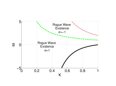
Figure 1: Existence domains of rogue waves in the plane $(\kappa,\omega)$, with $a=1$, in the focusing regime ($\sigma=1$) and defocusing regime ($\sigma=-1$). The red dotted line denotes $\omega=1/\kappa+1/\kappa^{3}$; green dashed line $\omega=1/\kappa$; black solid line $\omega=1/\kappa-1/\kappa^{3}$.

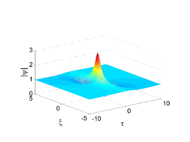
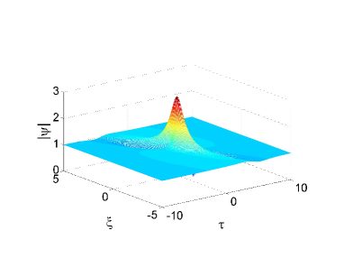
Figure 2: Typical rogue soliton states. Top, focusing regime $\sigma=1$, $\kappa=0.5$ and $a=1,\omega=0$. Bottom, defocusing regime $\sigma=-1$, $\kappa=0.5$ and $a=1,\omega=4$.

Let us turn our attention now to the linear stability analysis of the background solution of Eq.(1). A perturbed nonlinear background can be written as $\psi_{p}=[a+p]e^{i(\omega\tau-\beta\xi)}$, where $p(\xi,\tau)$ is a small complex perturbation that satisfies a linear differential evolution equation. Whenever $p$ is $\tau$-periodic with frequency $\Omega$, i.e., $p(\xi,\tau)=\eta_{s}(\xi)e^{i\Omega\tau}+\eta_{a}(\xi)e^{-i\Omega\tau}$, such equation reduces to a set of $2\times 2$ linear ordinary differential equations $\eta^{\prime}=iM\eta$, with $\eta=[\eta_{s},\eta^{*}_{a}]^{T}$ (here a prime stands for differentiation with respect to $\tau$). For any given real frequency $\Omega$, the generic perturbation $\eta(\xi)$ is a linear combination of exponentials $e^{iw_{j}\xi}$ where $w_{j},(j=1,2)$ are the two eigenvalues of the matrix $M=\{M_{ij}\}$, whose elements read as:

$$M_{11} =\frac{-\frac{1}{2}\Omega^{2}+\sigma a^{2}K-\Omega(\omega+\beta\kappa+\sigma a^{2}\kappa)}{(K-\kappa\Omega)},$$

$$M_{12} =\frac{\sigma a^{2}K}{(K-\kappa\Omega)},$$

$$M_{21} =-\frac{\sigma a^{2}K}{(K+\kappa\Omega)},$$

$$M_{22} =\frac{\frac{1}{2}\Omega^{2}-\sigma a^{2}K-\Omega(\omega+\beta\kappa+\sigma a^{2}\kappa)}{(K+\kappa\Omega)}.$$

Since the entries of the matrix M are all real, the eigenvalues $w_{j}$ are either real or they appear as complex conjugate pairs. The eigenvalues of the matrix $M$ are the roots of its characteristic polynomial,

$$B(w) =B_{2}w^{2}+B_{1}w+B_{0},$$ (3)

$$B_{2} =K^{2}-\kappa^{2}\Omega^{2},$$

$$B_{1} =-4\Omega(2\beta\kappa K+\kappa\Omega^{2}+2K\omega),$$

$$B_{0} =-\Omega^{2}+4[\beta^{2}\kappa^{2}+a^{4}\kappa^{2}+\omega^{2}+$$

$$2\beta\kappa(a^{2}\kappa\sigma+\omega)+A^{2}\sigma(K+2\kappa\omega).$$

Mi occurs whenever M has an eigenvalue $w$ with a negative imaginary part. Indeed, if the explosive rate is $G(\Omega)=-\textrm{Im}\{w\}>0$, perturbations grow exponentially like $\exp(G\xi)$ at the expense of the pump wave.

MI is well depicted by displaying the gain $G(\Omega)$ as function of $a,\omega,\sigma,\kappa$ and $\Omega$. The resulting MI gain spectrum is illustrated in Fig. 3 and Fig. 4.

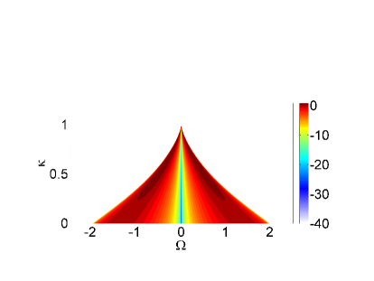
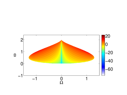
Figure 3: Maps of logaritmic MI gain ($10log_{10}G$) in the focusing ($\sigma=1$) FLE (1). Top, MI on the $(\Omega,\kappa)$ plane, calculated for the case $a=1,\omega=1$. Bottom, MI on the $(\Omega,\omega)$ plane, calculated for the case $a=1,\kappa=0.5$.

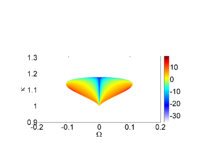
Figure 4: Maps of of logaritmic MI gain ($10log_{10}G$) in the defocusing ($\sigma=-1$) FLE (1). MI on the $(\Omega,\kappa)$ plane, calculated for the case $a=2,\omega=1$.

These figures show the MI gain in the focusing ans defocusing regime, respectively. In both cases, baseband MI is only present in a certain subset of the $\omega,\kappa$ parameters. Since the gain band (where $G(\Omega)\neq 0$) can be written as $0\leq\Omega_{1}<\Omega<\Omega_{2}$ (and its symmetric counterpart with respect to $\Omega=0$), baseband MI is obtained if $\Omega_{1}=0$, whereas passband MI occurs for $\Omega_{1}>0$.

We proceed next by focusing our attention on the MI gain spectrum, by evaluating the sign of the discriminant $\Delta$ of the characteristic polymomial (3): this leads to

$$sign\{\Delta\}=sign\{\Omega^{2}-4a^{2}\sigma K^{3}\left(1-a^{2}\kappa^{2}\sigma K\right)\}.$$ (4)

If the discriminant $\Delta$ is positive, the characteristic polynomial has two real roots and there is no MI. On the other hand if the discriminant $\Delta$ is negative, the characteristic polynomial $B$ has two complex conjugate roots, and Eq. (1) exhibits baseband MI. It is clear from Eq. (4) that for FLE if there is MI, it is of baseband type only: either the system is modulationally unstable for $\Omega\rightarrow 0$, either there is no MI at all. The interesting finding is that the sign constraint on the discriminant, which determines the presence of baseband MI, leads to the condition that $\omega$ should be in the range $[1/\kappa-1/(a^{2}\kappa^{3}),1/\kappa]$ in the focusing regime ($\sigma=1$), and in the range $[1/\kappa,1/\kappa+1/(a^{2}\kappa^{3})]$ in the defocusing regime ($\sigma=-1$). These conditions exactly coincide with the constraints that are required for the existence of the rogue wave solution (2).

These results are important since they show that, for both the focusing and the defocusing regime, rogue wave solutions of Eq. (1) only exist in the subset of the parameters space where also baseband MI is present.

We checked the results of our analysis by extensive numerical solutions of Eq. (1). These simulations indeed confirm that, in the baseband MI regime, multiple rogue waves can generated from an input plane wave background with a superimposed random noise seed (see Fig. 5).

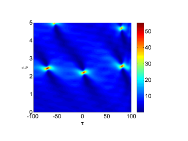
Figure 5: Color plot of $|\psi(\xi,\tau)|^{2}$ from the numerical solution of the focusing FLE (1) in the baseband MI regime. The initial condition is a plane wave perturbed by a random noise seed, with parameters: $a=2,\omega=1$, $\kappa=1.15,\sigma=-1$.

III Defocusing VNLSE

The defocusing VNLSE constitutes another model that has been thoroughly exploited for the description of fundamental physical phenomena in several different disciplines. In oceanography, for instance, it may describe the interaction of crossing currents miguel_crossing . In the context of nonlinear optics, it has been derived for the description of pulse propagation in randomly birefringent fibers meniuk , or coupled beam propagation in photorefractive media segev .

For our studies, we write the defocusing VNLSE in the following dimensionless form

$$\left\{\begin{array}[]{lll}i\psi^{(1)}_{\xi}+\psi^{(1)}_{\tau\tau}-2(|\psi^{(1)}|^{2}+|\psi^{(2)}|^{2})\psi^{(1)}&=&0\\ i\psi^{(2)}_{\xi}+\psi^{(2)}_{\tau\tau}-2(|\psi^{(1)}|^{2}+|\psi^{(2)}|^{2})\psi^{(2)}&=&0,\end{array}\right.$$ (5)

where $\psi^{(1)}(\xi,\tau),\,\psi^{(2)}(\xi,\tau)$ represent complex wave envelopes; $\xi,\tau$ are the propagation distance and the retarded time, respectively; each subscripted variable in Eqs. (5) stands for partial differentiation. Note that Eqs. (5) refer to the defocusing (or normal dispersion) regime. Unlike the case of the scalar NLSE, rational rogue solutions of the defocusing VNLSE do exist, as it was recently demonstrated baronio14 . These rogue wave solutions can be expressed as:

$$\psi^{(j)}=\psi_{0}^{(j)}\big{[}\frac{p^{2}\tau^{2}+p^{4}\xi^{2}+p\tau(\alpha_{j}+\beta\theta_{j})-i\alpha_{j}p^{2}\xi+\beta\theta_{j}}{p^{2}\tau^{2}+p^{4}\xi^{2}+\beta(p\tau+1)}\big{]}$$ (6)

with $j=1,2$. $\psi_{0}^{(j)}=a_{j}e^{i(\omega_{j}\tau-\beta_{j}\xi)}$, represent the background solution of Eqs. (5), $a_{j}$ are the real amplitude parameters ($a_{j}>0$), $\omega_{j}$ are the frequencies, and $\beta_{j}=\omega_{j}^{2}+2(a_{1}^{2}+a_{2}^{2})$.

Moreover, $\alpha_{j}=4p^{2}/(p^{2}+4\omega_{j}^{2}),\theta_{j}=(2\omega_{j}+ip)/(2\omega_{j}-ip);\beta=p^{3}/\chi(p^{2}+4\omega_{1}\omega_{2}),p=2\textrm{{Im}}(\lambda+k),\omega_{1}+\omega_{2}=2\textrm{{Re}}(\lambda+k),\omega_{1}-\omega_{2}=2\omega,\chi=\textrm{{Im}}k.$ The evaluation of the complex value of $\lambda$ and $k$ should be performed as follows. The parameter $\lambda$ is the double solution of the polynomial $A(\lambda)=\lambda^{3}+A_{2}\lambda^{2}+A_{1}\lambda+A_{0}=0$, with $A_{0}=-k^{3}+k(\omega^{2}+a_{1}^{2}+a_{2}^{2})+\omega(a_{2}^{2}-a_{1}^{2})$, $A_{1}=-k^{2}-\omega^{2}+a_{1}^{2}+a_{2}^{2}$, $A_{2}=k$. Moreover, the constraint on the double roots of $A(\lambda)$ is satisfied whenever the discriminant of $A(\lambda)$ is zero, which results in the fourth order polinomial condition $D(k)=k^{4}+D_{3}k^{3}+D_{2}k^{2}+D_{1}k+D_{0}=0$, with $D_{0}=(\omega^{2}-a_{1}^{2}-a_{2}^{2})^{3}/(2^{4}\omega^{2})-(3/4)^{3}(a_{2}^{2}-a_{1}^{2})^{2}$, $D_{1}=-9(a_{2}^{2}-a_{1}^{2})(2\omega^{2}+a_{1}^{2}+a_{2}^{2})/(2^{4}\omega)$, $D_{2}=-[8q^{4}-(a_{1}^{2}+a_{2}^{2})^{2}+20\omega^{2}(a_{1}^{2}+a_{2}^{2})]/(2^{4}\omega^{2})$, $D_{3}=(a_{2}^{2}-a_{1}^{2})/(2\omega)$. Thus, $\lambda$ is the double solution of the third order polynomial $A(\lambda)$, and $k$ is any strictly complex solution of the fourth order polynomial $D(k)$ (see Ref. baronio14 for details on nonlinear waves calculations and characteristics).

The rogue waves (6) depend on the real parameters $a_{1},a_{2}$ and $\omega$ which originate from the backgrounds: $a_{1},a_{2}$ represent the amplitudes, and $2\omega$ the “frequency” difference of the waves. Figure 6 shows a typical dark-bright solution (6).

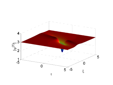
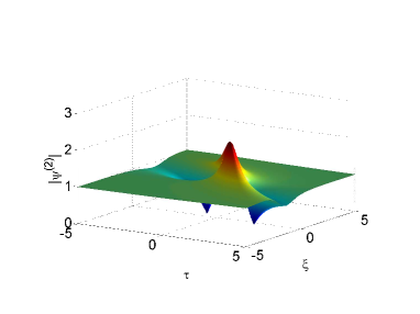
Figure 6: Rogue wave envelope distributions $|\psi^{(1)}(\tau,\xi)|$ and $|\psi^{(2)}(\tau,\xi)|$ of expression (6). Here, $a_{1}=3,a_{2}=1,\omega=1$. $k=2.36954+1.1972i$ and $\lambda=-1.69162-1.79721i$.

In the defocusing regime, it has been demonstrated baronio14 that rogue waves exist in the subset of parameters $a_{1},a_{2},\omega$ where

$$(a_{1}^{2}+a_{2}^{2})^{3}-12(a_{1}^{4}-7a_{1}^{2}a_{2}^{2}+a_{2}^{4})\omega^{2}+48(a_{1}^{2}+a_{2}^{2})\omega^{4}-64\omega^{6}>0.$$ (7)

Figure 7 illustrates two characteristic examples of the existence condition for rogue waves. In particular, Fig.7 shows that, for a fixed $\omega$, the background amplitudes should be sufficiently large in order to allow for rogue wave formation.

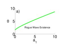
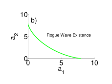
Figure 7: Rogue wave existence condition. a) $(\omega,a_{1})$ plane, with $a_{2}=3$. b) $(a_{2},a_{1})$ plane, with $\omega=4$.

Let us turn our attention now to the linear stability analysis of the background solution of Eqs.(5). A perturbed nonlinear background may be written as $\psi_{p}^{(j)}=[a_{j}+p_{j}]e^{i\omega_{j}\tau-i\beta_{j}\xi}$, where $p_{j}(\xi,\tau)$ are small complex perturbations that obey a linear partial differential equation. Whenever $p_{j}(\xi,\tau)$ are $\tau-$periodic with frequency $\Omega$, i.e., $p_{j}(\xi,\tau)=\eta_{j,s}(\xi)e^{i\Omega\tau}+\eta_{j,a}(\xi)e^{-i\Omega\tau}$, their equations reduce to the $4\times 4$ linear ordinary differential equation $\eta^{\prime}=iM\eta$, with $\eta=[\eta_{1,s},\eta^{*}_{1,a},\eta_{2,s},\eta^{*}_{2,a}]^{T}$ . For any given real frequency $\Omega$, the generic perturbation $\eta(\xi)$ may be expressed by a linear combination of exponentials $\exp(iw_{j}\xi)$ where $w_{j},\;j=1,\cdots,4,$ are the four eigenvalues of the matrix $M=\{M_{ij}\}$.

$$M_{11} =-\Omega^{2}-2\Omega\omega_{1}-2a_{1}^{2},$$

$$M_{22} =\Omega^{2}-2\Omega\omega_{1}+2a_{1}^{2},$$

$$M_{33} =-\Omega^{2}-2\Omega\omega_{2}-2a_{2}^{2},$$

$$M_{44} =\Omega^{2}-2\Omega\omega_{2}+2a_{2}^{2},$$

$$M_{12} =-M_{21}=-2a_{1}^{2},$$

$$M_{13} =M_{14}=M_{31}=M_{32}=-2a_{1}a_{2},$$

$$M_{41} =M_{23}=M_{24}=M_{42}=2a_{1}a_{2},$$

$$M_{43} =-M_{34}=2a_{2}^{2}.$$

Since the entries of the matrix $M$ are all real, the eigenvalues $w_{j}$ are either real or they appear as complex conjugate pairs. These eigenvalues are the roots of the characteristic polynomial $B(w)$ of the matrix $M$:

$$B(w) =w^{4}+B_{3}w^{3}+B_{2}w^{2}+B_{1}w+B_{0},$$

$$B_{0} =(\Omega^{2}-4\omega^{2})[4(a_{1}^{2}+a_{2}^{2}-\omega^{2})+\Omega^{2}]\Omega^{4},$$

$$B_{1} =16\omega(a_{1}^{2}-a_{2}^{2})\Omega^{3},$$

$$B_{2} =-2[2(a_{1}^{2}+a_{2}^{2}+2\omega^{2})+\Omega^{2}]\Omega^{2},$$

$$B_{3} =0.$$

MI occurs whenever $M$ has an eigenvalue $w$ with a negative imaginary part, $\textrm{Im}\{w\}<0$. Indeed, if the explosive rate is $G(\Omega)=-\textrm{Im}\{w\}>0$, initial perturbations grow exponentially as $\exp(G\xi)$ at the expense of the pump waves. Typical shapes of the MI gain $G(\Omega)$ are shown in Fig. 8.

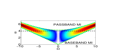
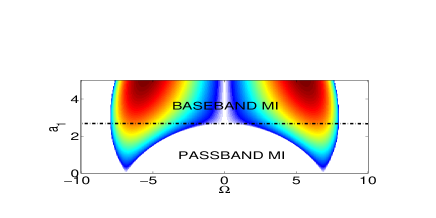
Figure 8: Maps of MI gain $2G$ of the VNLSE (5). a) MI on the $(\Omega,\omega)$ plane, calculated for the case $a_{1}=3,a_{2}=3$, $\omega_{1}=-\omega_{2}=\omega$. Dotted (green online) curves represent the analytical marginal stability condition $\Omega=2\omega$, $\Omega^{2}=\textrm{max}\{4\omega^{2}-8a^{2},0\}$. b) MI on the $(\Omega,a_{1})$ plane, calculated for the case $a_{2}=3,\omega_{1}=-\omega_{2}=4$.

Figure 8(a) corresponds to the case where the nonlinear background modes have opposite frequencies ($\omega_{1}=-\omega_{2}=\omega$). The higher $\omega$, the higher $G$. In the special case of equal background amplitudes $a_{1}=a_{2}=a$, the marginal stability conditions can be analytically found: $\Omega^{2}=4\omega^{2}$, $\Omega^{2}=\textrm{max}\{4\omega^{2}-8a^{2},0\}$. Thus, for $a^{2}>\omega^{2}/2$ a baseband MI, which includes frequencies that are arbitrarily close to zero, is present (i.e. $0<\Omega^{2}<4\omega^{2}$). Instead, for $a^{2}\leq\omega^{2}/2$, MI only occurs for frequencies within the passband range $(4\omega^{2}-8a^{2})<\Omega^{2}<4\omega^{2}$. We may point out that the rogue waves (6) necessarily exist for $a^{2}>\omega^{2}/2$. Thus, rogue waves (6) and baseband MI coexist.

Figure 8(b) illustrates the case of different frequencies ($\omega_{1}=-\omega_{2}=\omega$) and input amplitudes $a_{1}\neq a_{2}$ for the nonlinear background modes. For low values of $a_{1}$, only passband MI is present. By increasing $a_{1}$, the baseband MI condition is eventually attained.
In order to analytically represent the condition for the occurrence of baseband MI, let us consider the limit $\Omega\rightarrow 0$. To this aim, we may rewrite the characteristic polynomial as $B(\Omega v)=\Omega^{4}b(v)$, and consider the polynomial $b(v)$ at $\Omega=0$, namely $b(v)=v^{4}+b_{3}v^{3}+b_{2}v^{2}+b_{1}v+b_{0}$, $b_{0}=-16\omega^{2}(a_{1}^{2}+a_{2}^{2}-\omega^{2})$, $b_{1}=16q(a_{1}^{2}-a_{2}^{2})$, $b_{2}=-4(a_{1}^{2}+a_{2}^{2}+2\omega^{2})$, $b_{3}=0$. Let us evaluate now the discriminant of the characteristic polynomial $B$: if the discriminant is positive, $B$ has four real roots, and no MI occurs. Whereas if the discriminant of $B$ is negative, there are two real roots and two complex conjugate roots, and Eqs.(5) exhibits baseband MI. Again, the interesting finding is that the constraint on the sign of the discriminant of the characteristic polynomial $B$, which leads to the baseband MI condition, turns out to exactly coincide with the sign constraint (7) that is required for rogue wave existence.

Thus we may conclude that in the defocusing regime, rogue wave solutions (6) only exist in the subset of the parameter space where MI is present, and in particular if and only if baseband MI is present.

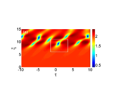
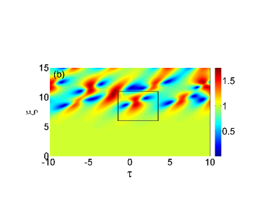
Figure 9: Color plot of $|\psi^{(1)}(\tau,\xi)|$ (a) and $|\psi^{(2)}(\tau,\xi)|$ (b) from the numerical solution of the defocusing VNLSE. The initial condition is a plane wave perturbed by weak random noise. Parameters: $a_{1}=2,a_{2}=1,\omega=1$. A rogue wave is highlighted by a surrounding box.

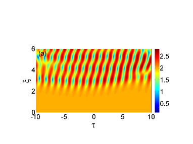
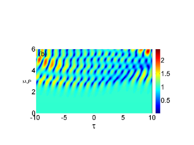
Figure 10: Color plot of $|\psi^{(1)}(\tau,\xi)|$ (a) and $|\psi^{(2)}(\tau,\xi)|$ (b) from the numerical solution of the defocusing VNLSE. The initial condition is a plane wave perturbed by weak random noise. Parameters: $a_{1}=2,a_{2}=1,\omega=3$. No rogue waves are generated in this case.

Fig. 9 and Fig. 10 show two different numerically computed nonlinear evolutions, obtained in the case of baseband MI (leading to rogue wave generation) and of passband MI, respectively. These evolutions permit to highlight that the nonlinear evolution of baseband MI leads to rogue wave solutions of the VNLSE (5) . Figure 9 shows the numerically computed evolution of a plane wave perturbed by a small random noise in the baseband MI regime. After a first initial stage of linear growth of the unstable frequency modes, for $\xi>5$ the nonlinear stage of MI is reached. As we can see, MI leads to the formation of multiple isolated peaks (dips) that emerge at random positions. By carefully analyzing one of these peaks, for example the peak near the point ($\tau=0,\xi=9$), we may clearly recognize the shape of a rogue wave as it is described by the expression (6). Conversely, Fig.10 shows the numerically computed evolution of a plane wave perturbed by a small random noise, in the passband MI regime. After a first initial stage of linear growth of the unstable frequency modes, for $\xi>2$ the nonlinear stage of MI is reached. In this case, we may observe the generation of a train of nonlinear oscillations, with wave-numbers corresponding to the peak of MI gain ($\Omega_{max}=5$). As it was expected, no isolated peaks (dips) emerge from noise in this case, given that the condition for the existence of rogue waves is not verified.

IV LWSW model

The last model we consider in our survey is the LWSW resonance. It is as well a general model that describes the interaction between a rapidly varying wave and a quasi continuous one. In optics the LWSW resonance rules wave propagation in negative index media tataronis08 or the optical-microvave interactions bubke03 . Whereas in hydrodynamics the LWSW resonance results from the interaction between capillary and gravity waves djordjevic77 .

For our studies, we write the LWSW equations in the dimensionless form

$$\left\{\begin{array}[]{lll}i\psi^{(S)}_{\xi}&+&\frac{1}{2}\psi^{(S)}_{\tau\tau}+\psi^{(L)}\psi^{(S)}=0\\ \psi^{(L)}_{\xi}&-&|\psi^{(S)}|^{2}_{\tau}=0,\end{array}\right.$$ (8)

where $\psi^{(S)}(\xi,\tau)$ represents the short wave complex envelope, and $\psi^{(L)}(\xi,\tau)$ represents the long wave real field; $\xi$ and $\tau$ are the propagation distance and the retarded time, respectively; each subscripted variable stands for partial differentiation.

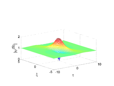
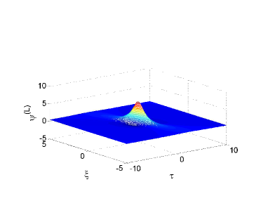
Figure 11: Rogue wave envelope distributions $|\psi^{(S)}(\tau,\xi)|$ and $|\psi^{(L)}(\tau,\xi)|$ corresponding to expressions (8). Here, $a=1,\omega=0,b=0.5$.

The fundamental rogue wave solution of Eqs. (8) has recently been reported in Ref.chen14R , and reads as

$$\psi^{(S)}=\psi_{0}^{(S)}\big{[}1-\frac{i\xi+\frac{i\tau}{2m-\omega}+\frac{1}{2(2m-\omega)(m-\omega)}}{(\tau-m\xi)^{2}+n^{2}\xi^{2}+1/4n^{2}}\big{]},$$

$$\psi^{(L)}=b+\frac{n^{2}\xi^{2}-(\tau-m\xi)^{2}+1/4n^{2}}{[(\tau-m\xi)^{2}+n^{2}\xi^{2}+1/4n^{2}]^{2}},$$ (9)

where $\psi_{0}^{(S)}=ae^{i(\omega\tau-\beta\xi)}$ represents the background solution of the short wave, defined by the amplitude $a$ ($a>0$), frequency $\omega$, and wave number $\beta=\omega^{2}/2-b$; the amplitude $b$ ($b\geq 0$) defines the background solution of the coupled long wave real field. The parameters $m$ and $n$ are real, defined by $m=\frac{1}{6}[5\omega-\sqrt{3(\omega^{2}+l+\upsilon/l)}]$, $n=\pm\sqrt{(3m-\omega)(m-\omega)}$, with $\upsilon=\frac{1}{9}\omega^{4}+6\omega a^{2}$, $\rho=\frac{1}{2}\omega^{6}-\frac{1}{54}(27a^{2}+5\omega^{3})^{2}$. $l=-(\rho-\sqrt{\rho^{2}-\upsilon^{3}})^{1/3}$, for $\omega\leq-3(2a^{2})^{1/3}$, and $l=(-\rho+\sqrt{\rho^{2}-\upsilon^{3}})^{1/3}$, for $-3(2a^{2})^{1/3}<\omega\leq\frac{3}{2}(2a^{2})^{1/3}$. LWSW rogue waves (9) depend on the real parameters $a$, $\omega$ and $b$ (see Ref. chen14R for details on nonlinear wave characteristics). Figure 11 shows a typical LWSW rogue solution. Importantly, the existence condition for rogue waves of the LWSW model is that $\omega\leq\frac{3}{2}(2a^{2})^{1/3}$.

Let us turn our attention now to the linear stability analysis of the background solution of Eqs. (8). Here a perturbed nonlinear background can be written as $\psi_{p}^{(S)}=[a+p_{S}]e^{i\omega\tau-i\beta\xi}$, and $\psi_{p}^{(L)}=b+p_{L}$ where $p_{S}(\xi,\tau),p_{L}(\xi,\tau)$ are small complex perturbations that obey linear partial differential equations. Whenever the perturbations $p_{S},p_{L}$ are $\tau-$periodic with frequency $\Omega$, i.e., $p_{S}(\xi,\tau)=\eta_{s}(\xi)e^{i\Omega\tau}+\eta_{a}(\xi)e^{-i\Omega\tau}$, and recalling that $\psi_{p}^{(L)}$ is real, $p_{L}(\xi,\tau)=g(\xi)e^{i\Omega\tau}+g^{*}(\xi)e^{-i\Omega\tau}$, the perturbation equations reduce to a $3\times 3$ linear ordinary differential equation $\eta^{\prime}=iM\eta$, with $\eta=[\eta_{s},\eta^{*}_{a},g]^{T}$ (here a prime stands for differentiation with respect to $\tau$). For any given real frequency $\Omega$, the generic perturbation may be expressed as a linear combination of exponentials $\exp(iw_{j}\xi)$ where $w_{j},\;j=1,\cdots,3,$ are the three eigenvalues of the matrix:

$$M=\left[\begin{array}[]{ccc}-\frac{1}{2}\Omega^{2}-\omega\Omega&0&a\\ 0&\frac{1}{2}\Omega^{2}-\omega\Omega&-a\\ \Omega a&\Omega a&0\end{array}\right].$$ (10)

Since the entries of the matrix $M$ are all real, the eigenvalues $w_{j}$ are either real, or they appear as complex conjugate pairs. These eigenvalues are obtained as the roots of the characteristic polynomial $B(w)$ of the matrix $M$:

$$B(w) =B_{3}w^{3}+B_{2}w^{2}+B_{1}w+B_{0},$$ (11)

$$B_{0} =a^{2}\Omega^{3},\;\;B_{1}=\omega^{2}\Omega^{2}-\Omega^{4}/4,\;\;B_{2}=2\omega\Omega,\;\;B_{3}=1.$$

MI occurs whenever $M$ has an eigenvalue $w$ with a negative imaginary part, i.e., $\textrm{Im}\{w\}<0$. Indeed, if the explosive rate is $G(\Omega)=-\textrm{Im}\{w\}>0$, perturbations grow larger exponentially like $\exp(G\xi)$ at the expense of the pump waves. By calculating the discriminant of the polynomial $B$, one finds $\Delta=\Omega^{6}(\frac{1}{16}\Omega^{6}-\frac{1}{2}\Omega^{4}-\omega(9a^{2}-\omega^{3})\Omega^{2}+4a^{2}\omega^{3}-27a^{4})$. If the discriminant $\Delta$ is positive, the polynomial $B$ has real roots, and no MI occurs. Conversely if the discriminant $\Delta$ is negative, the polynomial $B$ has two complex conjugate roots, which means that MI is present for Eqs.(8). The marginal stability curves, corresponding to $\Delta=0$, can thus be calculated. Figure 12 shows a typical MI gain spectrum of the LWSW Eqs. (8): as one can see, there exist regions of either baseband or passband MI.

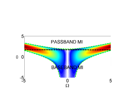
Figure 12: Maps of MI gain $2G$ of the LWSW Eqs. (8). MI on the $(\Omega,\omega)$ plane, calculated for the case $a=1$, Dashed (green online) curves represent the analytical marginal stability condition $\Omega^{6}(\frac{1}{16}\Omega^{6}-\frac{1}{2}\Omega^{4}-\omega(9a^{2}-\omega^{3})\Omega^{2}+4a^{2}\omega^{3}-27a^{2})=0$.

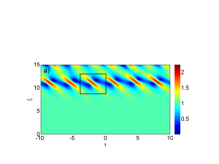
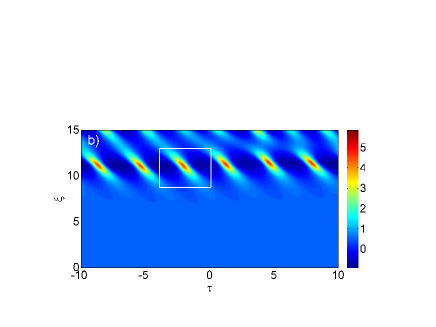
Figure 13: Color plot of $|\psi^{(S)}(\tau,\xi)|$ (a) and $|\psi^{(L)}(\tau,\xi)|$ (b) from the numerical solution of the LWSW equation. The initial condition is a plane wave perturbed by weak random noise. Parameters: $a=1,B=0.5,\omega=0$. A rogue wave is highlighted by a surrounding box.

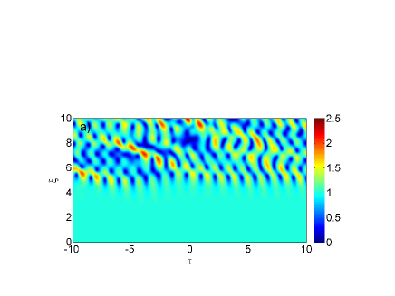
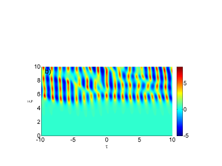
Figure 14: Color plot of $|\psi^{(S)}(\tau,\xi)|$ (a) and $|\psi^{(L)}(\tau,\xi)|$ (b) from the numerical solution of the LWSW equation. The initial condition is a plane wave perturbed by weak random noise. Parameters: $a=1,B=0.5,\omega=2.5$. No rogue wave is generated in this case.

As in previous sections, let us proceed now to discuss the MI behavior in the limit situation where $\Omega\rightarrow 0$, a condition which characterizes the occurrence of baseband MI. In this regime, the discriminant of the polynomial $B$ reduces to $\Delta=4a^{2}\omega^{3}-27a^{4}$, which leads to the MI condition $\omega<\frac{3}{2}(2a^{2})^{1/3}$. Again, the baseband MI condition turns out to exactly coincide with the condition for the existence of rogue wave solutions of Eqs. (8).

Figure 14 shows a numerical solution of LWSW, obtained in the case of baseband MI (leading to rogue wave generation), showing the evolution of a plane wave perturbed by a small random noise. After a first initial stage of linear growth of the unstable frequency modes, for $\xi>8$ the nonlinear stage of MI is reached. As we can see, MI leads to the formation of multiple isolated peaks that emerge at random positions. By carefully analyzing one of these peaks, we may clearly recognize the shape of a rogue wave as it is described by the expression (IV).

V Conclusions

In this work we studied the existence and the properties of rogue wave solutions in different integrable nonlinear wave evolution models which are of widespread use both in optics and in hydrodynamics. Namely, we considered the Fokas-Lenells equation, the defocusing vector nolinear Schrödinger equation and the long-wave-short-wave resonance. We found out that in all of these models rogue waves, which can be modeled as rational solutions, only exist in the subset of parameters where MI is present, but if and only if the MI gain band also contains the zero-frequency perturbation as a limiting case (baseband MI). We have numerically confirmed that in the baseband-MI regime rogue waves can indeed be excited from a noisy input cw background. Otherwise, when there is passband MI we only observed the generation of nonlinear wave oscillations. Based on the above findings, we are led to believe that the conditions for simultaneous rogue wave existence and of baseband MI may also be extended to other relevant and integrable and non-integrable physical models of great interest for applications, for instance consider frequency conversion models baro10 ; confo12 where extreme wave events and complex breaking beaviours are known to place confo06 ; confo13 .

References

- (1) , Nature 430, 492 (2004).
- (2) S. Perkins, Science News 170, 328 (2006).
- (3) E. Pelinovsky and C. Kharif, Extreme Ocean Waves (Springer, Berlin, 2008).
- (4) C. Kharif, E. Pelinovsky, and A. Slunyaev, Rogue Waves in the Ocean (Springer, Heidelberg, 2009).
- (5) J. M. Dudley, F. Dias, M. Erkintalo, and G. Genty, Nat. Photon. 8, 755 (2014).
- (6) M. Onorato, S. Residori, U. Bortolozzo, A. Montina, and F.T. Arecchi, Phys. Rep. 528, 47 (2013).
- (7) D.H. Peregrine, J. Australian Math. Soc. Ser. B 25, 16 (1983).
- (8) B. Kibler, J. Fatome, C. Finot, G. Millot, F. Dias, G. Genty, N. Akhmediev, and J.M. Dudley, Nat. Phys. 6, 790 (2010).
- (9) A. Chabchoub, N.P. Hoffmann, and N. Akhmediev, Phys. Rev. Lett. 106, 204502 (2011).
- (10) H. Bailung, S.K. Sharma, and Y. Nakamura, Phys. Rev. Lett. 107, 255005 (2011).
- (11) C. Lecaplain, Ph. Grelu, J.M. Soto-Crespo, and N. Akhmediev, Phys. Rev. Lett. 108, 233901 (2012).
- (12) A. Ankiewicz, J.M. Soto-Crespo and N. Akhmediev, Phys. Rev. E 81, 046602 (2010).
- (13) U. Bandelow and N. Akhmediev, Phys. Rev. E 86, 026606 (2012).
- (14) S. Chen and L. Y. Song Phys. Lett. A 378, 1228 (2014).
- (15) F. Baronio, A. Degasperis, M. Conforti, and S. Wabnitz, Phys. Rev. Lett. 109, 044102 (2012).
- (16) L.C. Zhao and J. Liu, Phys. Rev. E 87, 013201 (2013).
- (17) B.G. Zhai, W.G. Zhang, X.L. Wang, H.Q. Zhang, Schrödinger equations,” Nonlinear Anal-Real 14, 14-27 (2013).
- (18) F. Baronio, M. Conforti, A. Degasperis, S. Lombardo, M. Onorato, and S. Wabnitz, Phys. Rev. Lett. 113, 034101 (2014).
- (19) F. Baronio, M. Conforti, A. Degasperis, and S. Lombardo, Phys. Rev. Lett. 111, 114101 (2013).
- (20) S. Chen and L. Y. Song, Phys. Rev. E 87, 032910 (2013).
- (21) S. Chen, Ph. Grelu, and J.M. Soto-Crespo, Phys. Rev. E 89, 011201(R) (2014).
- (22) V. E. Zakharov and L. A. Ostrovsky, Physica D 238, 540 (2009).
- (23) M.S. Ruderman, Eur. Phys. J. Special Topics 185, 57 (2010).
- (24) A. Sluniaev, Eur. Phys. J. Special Topics 185, 67 (2010).
- (25) C. Kharif and J. Touboul, Eur. Phys. J. Special Topics 185, 159 (2010).
- (26) A. S. Fokas, Physica D 87, 145 (1995).
- (27) J. Lenells, Stud. Appl. Math. 123, 215 (2009).
- (28) M. Onorato, A. R. Osborne, and M. Serio, Phys. Rev. Lett. 96, 014503 (2006).
- (29) P. K. A. Wai and C. R. Menyuk, J. Lightwave Technol. 14, 148 (1996).
- (30) Z. Chen, M. Segev, T. H. Coskun, D. N. Christodoulides, and Y. S. Kivshiar, J. Opt. Soc. Am. B 11, 3066 (1997).
- (31) A. Chowdhury and J. A. Tataronis, Phys. Rev. Lett. 100, 153905 (2008).
- (32) K. Bubke, D. C. Hutchings, U. Peshel, and F. Lederer, Phys. Rev. E 67, 016611 (2003).
- (33) V. D. Djordjevic and L. G. Redekopp, J. Fluid Mech. 79, 703 (1977).
- (34) F. Baronio, M. Conforti, C. De Angelis, A. Degasperis, M. Andreana, V. Couderc, and A. Barthelemy, Phys. Rev. Lett. 104, 113902 (2010).
- (35) M. Conforti, F. Baronio, and S. Trillo, Opt. Lett. 37, 1082-1084 (2012).
- (36) M. Conforti, F. Baronio, A. Degasperis, and S. Wabnitz, Phys. Rev. E 74, 065602 (2006).
- (37) M. Conforti, F. Baronio, and S. Trillo, Opt. Lett. 38, 1648 (2013).