Simulation of X-ray diffraction profiles for bent anisotropic crystals

Abstract

The equations for calculating diffraction profiles for bent crystals are revisited for both meridional and sagittal bending. Two approximated methods for computing diffraction profiles are treated: multilamellar and Penning-Polder. A common treatment of crystal anisotropy is included in these models. The formulation presented is implemented into the XOP package, completing and updating the crystal module that simulates diffraction profiles for perfect, mosaic and now distorted crystals by elastic bending.

The equations for simulating diffraction profiles and their implementation in computer code are presented for the cases of meridional and sagittal bent crystals using the multilamellar and Penning-Polder theories and including crystal anisotropy.

1 Introduction

The motivation of this work is the availability of easy-to-use computer codes for simulating diffraction or reflection profiles of bent crystals. The target audience is the users and researchers of synchrotron radiation facilities, but also other fields of X-ray research, like plasma physics. There is a vast literature on the theory and applicability of the Dynamical Theory of Diffraction to the calculation of diffraction profiles (see e.g, [Authier] for an updated review). However, many scientists and engineers need to know the performances of bent crystals under X-rays without becoming specialist in the field of Dynamical Diffraction. Several available codes may be used, many of them available via collaborations with their authors: REFLECT [REFLECT], REFLEX [Caciuffo], PEPO [Schulze], DIXI [DIXI], and others publically available [Stepanov]. One popular code for the synchrotron community is XOP [Xop2011], a graphical environment for computer codes for i) modeling of X-ray sources (e.g., synchrotron radiation sources, such as undulators and wigglers), ii) calculating characteristics of optical elements (mirrors, filters, crystals, multilayers, etc.), and iii) multipurpose data visualizations and analyses. XOP is used extensively to simulate crystal diffraction profiles for perfect, bent, and mosaic crystals.

The calculation of diffraction profiles for flat (undistorted) crystals is usually performed using the basic equations of the Dynamical Theory, in different formulations. Although a full quantum treatment of X-ray diffraction by a crystal exists [ashkin, kuriyama], a classical approach, as discussed in [hartwig_hierarchy] is adopted for most practical cases. In the classical approach, the propagation of the X-ray field inside and outside the crystal is described by the Maxwell equations assuming that all quantities (electric susceptibility, electric field, etc.) are defined in a continuous way for any point in the space and time, and the interaction of the X-ray field with the crystal electrons is described by quantum mechanics. The dynamical theories for X-ray diffraction in perfect crystals have been extended to include lattice distortions related to crystalline defects and macroscopic bending. For practical purposes, several levels of approximations may be defined [hartwig_hierarchy]:

1. dynamical diffraction theory for the perfect crystal,

2. local applications of the dynamical theory for perfect crystals to distorted ones,

3. geometrical optics or eikonal theory, and

4. wave optics or Takagi theory.

Item (a) is related to the classical dynamical diffraction of X-rays in perfect crystals. The term dynamical is used when the rescattering and absorption of the X-rays in the crystal volume is considered. Perfect crystals are ideal undistorted monocrystals over a large distances (as compared with the unit cells) thus assuming perfect alignment of the atoms in the crystalline structure. There is no curvature of the atomic planes (like the originated by elastic bending or thermal distortion) and no alteration of the atomic order (no inclusions, dislocations, defects, stress, cracks, etc). Since the pioneering work of [Darwin14], several several formulations are available [Ewald17], [Laue31], [Zachariasen], etc. Some comprehensive books describe them [James], [Pinsker] and [Authier], which includes a complete historical review.

The (b) approximation works for crystals with small distortions with respect to the perfect crystals. This means that the displacement vector $\vec{u}(\vec{r})$ varies very slowly. The crystal deformation transforms a point with position $\vec{r}$ into another at $\vec{r^{\prime}}$, with $\vec{u}(\vec{r})=\vec{r^{\prime}}-\vec{r}\approx\vec{u}(\vec{r^{\prime}})$). The crystal reflectivity for diffracted beam can therefore be computed quantitatively by shifting the angular position of the incident direction by a value equal to the effective misorientation, and applying the diffracted intensity of the perfect crystal. This method was introduced by [Bonse] and [Authier1966]. Also, the multilamellar method [Caciuffo, Erola] discussed later belongs to this category. It can be used for estimating the diffraction profile in both Bragg and Laue geometries in many practical cases of crystal curvature.

The diffraction theory of the (c) approximation mimics the geometrical optics for visible light. An inductive derivation was made by [Penning], a deductive theory was presented in [Kato1, Kato2, Kato3], and a derivation from the Takagi-Taupin Equations is in [IndenbomLevel3]. Level (d) rely on the Takagi-Taupin equations [Takagi, Taupin].

For calculations of perfect undistorted crystals XOP implements the equations of the dynamical theory of diffraction from [Zachariasen], summarized in Section 2.1. On the other hand, imperfect mosaic crystals can be simulated in XOP also using Zachariasen theory which is valid for mosaicity values much larger than the Darwin width.

In this work we extended the XCRYSTAL application in XOP to cover perfect crystals with small deformations originated by elastic bending. Elastic bending produces a crystal distortion that depends on its anisotropy. Every crystalline material is anisotropic, meaning the the elastic constants are not scalar, but depend on the direction (they are deduced from the compliance or stiffness tensors). Anisotropy is important when the crystal is bent, and is not relevant for the perfect undistorted crystals. We distinguish curvature in two directions with respect to the direction of the incident beam: meridional curvature in a plane that contains the incident direction, and sagittal, a plane perpendicular to it. The meridional plane coincides with the diffraction plane. A cylindrically bent crystal is curved in one single plane. A single moment is sufficient to bent the crystal in one direction. Two moments along perpendicular planes will bend the crystal in two directions. Perfect cylinders are difficult to obtain by elastic bending, because when applying one-moment to a crystal block or plate there is an spurious curvature in the plane perpendicular to the main bending plane (anticlastic curvature). Spherical or toroidal crystals are curved in both planes, usually made by applying two moments. The elastic constants and tensors are related to the principal crystallographic directions, which are coincident with the crystal block directions only if the crystals is symmetric. i.e., the crystalline planes are parallel to the crystal faces. In the most general case, the crystal planes are not parallel to the crystallographic directions and the crystal is called asymmetric. For the diffraction effects, a crystal curved with a non constant radius of curvature (parabolic, ellipsoidal, conic, etc.) can be approximated as a crystal with two averaged curvatures over the meridional and sagittal planes.

For simulating the diffraction profiles, two approximated theories are used: the multilamellar method and the Penning-Polder theory.

The multilamellar method described in Section 2.2 can be used to simulate diffraction profiles of curved crystals in both Bragg and Laue geometries. This models belongs to level of approximation (b). We develop the formulation of the multilamellar theory working for both sagittal and meridional curvatures in both Bragg and Laue geometries. This requires a correct treatment of the crystal anisotropy. The unified formulation presented here extends the cases treated in literature for isotropic Bragg crystals like [Caciuffo, Erola] and for anisotropic Laue crystals [xianbo_spie] to the general case of two-moment bending Laue or Bragg anisotropic crystals.

The Penning-Polder model [Penning] summarized in Section 2.3 belongs to the level of approximations (c), and only applies to Laue geometry. This model has been successfully applied for calculating the diffraction profiles of high energy monochromators used in beamlines at many synchrotrons (APS, NSLS, ESRF, Spring-8, Petra, Diamond, etc.). Again, we present here a formulation that can be applied for crystals bent in two directions (meridional and sagittaly, thus unifying previous uses of the Penning-Polder theory for meridionally bent crystals, isotropic [Sanchez1997] or anisotropic [Schulze], or for sagittal bending [xianbo_spie]. Approximation level (d), thus solving Takagi-Taupin equations will be addressed in a future work.

From the computer point of view, a unification of and modernization of the XOP crystal module has been done in order to upgrade, clean and improve its structure. A single Fortran 95 module calculates now crystal diffraction using the different calculation algorithms described here, using a full 3D vectorial calculus for beam direction and crystal orientation. Thus, this paper is a good companion of the software package and will be used as reference manual. It is designed for being integrated in other X-ray codes, like for the ray tracing package SHADOW [SHADOW].

2 Algorithms for computing diffraction by bent crystals

Using a crystal reflection defined by the Miller indices $hkl$, the reciprocal vector of the lattice is $\vec{H}=(1/d_{hkl})\vec{n}^{H}$, with $d_{hkl}$ the interplanar distance, and $\vec{n}^{H}$ a unitary vector normal to the Bragg planes [$hkl$].

The Laue equation

$$\vec{k}^{H}_{B}=\vec{k}^{0}_{B}+\vec{H},$$ (1)

which is satisfied only for the diffraction condition, gives the wavevector of the diffracted wave $\vec{k}^{H}_{B}$ for a particular position of the incident wavevector $\vec{k}^{0}_{B}$, that is, its angle with the reflecting $[hkl]$ planes is the Bragg angle $\theta_{B}$. This gives the Bragg law $\lambda=2d_{hkl}\sin\theta_{B}$, with $\lambda$ the photon wavelength. In this paper $|\vec{k}|=1/\lambda$ as in the text of [Zachariasen].

The change in the direction of any monochromatic beam (not necessarily satisfying the diffraction condition or Laue equation) diffracted by a crystal (Laue or Bragg) can be calculated using i) elastic scattering in the diffraction process:

$$|\vec{k^{0}}|=|\vec{k^{H}}|=\frac{1}{\lambda},$$ (2)

with $\vec{k}^{0,H}=(1/\lambda)\vec{V}^{0,H}$, and $\vec{V}$ a unitary vector; and ii) the boundary conditions at the crystal surface:

$$\vec{k}^{H}_{||}=\vec{k}^{0}_{||}+\vec{H}_{||},$$ (3)

where $||$ refers to the component parallel to the crystal surface.

A crystal cut is defined by $\vec{n}$, a unity vector normal to the crystal surface pointing outside the crystal bulk. Usually it is expressed as a function of $\alpha$ in Bragg geometry, and $\chi$ in Laue geometry, but if both values are well-defined they can be used indistinctly in both geometries (see Appendix A). The projections of the beam directions onto this vector are: $\gamma_{0}=\vec{n}~{}\cdot~{}\vec{V^{0}}$ and $\gamma_{H}=\vec{n}~{}\cdot~{}\vec{V^{H}}$. The asymmetry factor is $b=(\vec{n}\cdot\vec{k^{0}})/(\vec{n}\cdot(\vec{k^{0}}+\vec{H}))\approx\gamma_{0}/\gamma_{H}$.

2.1 The perfect crystal

For the perfect (undistorted) crystal we follow the [Zachariasen] formulation, because of its accuracy, compactness and easy numerical implementation. This formulation expresses the crystal reflectivity as a function of angular parameter:

$$\alpha_{Z}=\frac{1}{|\vec{k}^{0}|^{2}}\left[|\vec{H}|^{2}+2\vec{k}^{0}~{}.~{}\vec{H}\right]$$ (4)

which measures the separation of the incident field from the Bragg condition either in angular terms (“rotating crystal”, for a fixed photon wavelength):

$$\alpha_{Z}\approx 2(\theta_{B}-\theta)\sin(2\theta_{B})=-2\Delta\theta\sin(2\theta_{B}),$$ (5)

or in terms of photon wavelength (or energy): (“Laue method”)

$$\alpha_{Z}\approx 4\frac{\lambda-\lambda_{B}}{\lambda_{B}}\sin^{2}\theta_{B}=4\frac{E_{B}-E}{E_{B}}\sin^{2}\theta_{B},$$ (6)

However, it is recommended to compute $\alpha_{Z}$ using the exact expression in Eq. (4) which is also valid in extreme cases, like in normal incidence.

The X-ray reflectivity of a single perfect parallel-sided crystal in Bragg (or reflection) geometry is:

$$r^{bragg}(\alpha_{Z})\equiv\frac{1}{|b|}\frac{I^{H}}{I^{0}}=\frac{1}{|b|}\left|\frac{x_{1}x_{2}(c_{1}-c_{2})}{c_{2}x_{2}-c_{1}x_{1}}\right|^{2}.$$ (7)

For Laue (or transmission) geometry we have:

$$r^{laue}(\alpha_{Z})\equiv\frac{1}{|b|}\frac{I^{H}}{I^{0}}=\frac{1}{|b|}\left|\frac{x_{1}x_{2}(c_{1}-c_{2})}{x_{2}-x_{1}}\right|^{2}.$$ (8)

The transmitivity (forward diffracted beam) are

$$t^{bragg}(\alpha_{Z})=\left|\frac{c_{1}c_{2}(x_{2}-x_{1})}{c_{2}x_{2}-c_{1}x_{1}}\right|^{2},$$ (9)

$$t^{laue}(\alpha_{Z})=\left|\frac{x_{2}c_{1}-x_{1}c_{2}}{x_{2}-x_{1}}\right|^{2},$$ (10)

$I^{0}$ is the intensity of the incident wave along direction $\vec{V^{0}}$ with wavevector $\vec{k^{0}}$ , $I^{H}$ is the intensity of the external diffracted wave along the direction $\vec{V^{H}}$ with wavevector $\vec{k^{H}}$ , $c_{1,2}$ are phase terms dependent on the crystal thickness $T$, and both $x_{1,2}$ and $c_{1,2}$ terms depend on $\alpha_{Z}$ and on the crystal electrical susceptibility in a rather non-trivial way:

$$\left(\begin{array}[]{ll}x_{1}\\ x_{2}\end{array}\right)=\frac{-z\pm\sqrt{qP^{2}+z^{2}}}{P\Psi_{\bar{H}}},$$ (13)

$$z=\frac{1-b}{2}\Psi_{0}+\frac{b}{2}\alpha_{Z},$$ (14)

$q=b\Psi_{H}\Psi_{\bar{H}}$, $P$ is the polarization factor ($P=1$ for $\sigma$-polarization, $P=|\cos 2\theta_{B}|$ for $\pi$-polarization), and $\Psi_{H}$ is the Fourier component of the electrical susceptibility $\Psi_{0}$ related to the structure factor $F_{H}$ as:

$$\Psi_{H}=\frac{-r_{0}\lambda^{2}}{\pi v_{c}}F_{H};~{}~{}~{}r_{0}=\frac{e^{2}}{mc^{2}},$$ (15)

where $r_{0}$ the classical electron radius, $v_{c}$ the volume of the unit cell, $e$ the charge of the electron and $c$ the speed of light.

The $c_{1,2}$ phases in Eqs. 7-10 are expressed as:

$$c_{1}=e^{-i\phi_{1}T}$$

$$c_{2}=e^{-i\phi_{2}T}$$

$$\phi_{1}=-\frac{2\pi k^{0}\delta^{\prime}_{0}}{\gamma_{0}}$$ (16)

$$\phi_{2}=-\frac{2\pi k^{0}\delta^{\prime\prime}_{0}}{\gamma_{0}}$$

and the other quantities are defined as:

$$\left(\begin{array}[]{ll}\delta_{0}^{\prime}\\ \delta_{0}^{\prime\prime}\end{array}\right)=\frac{1}{2}\left(\Psi_{0}-z\pm\sqrt{qP^{2}+z^{2}}\right),$$ (19)

Note that a factor $|b|^{-1}$ appears for calculating the diffracted beams (Eqs. (7) and (8)) to guarantee the conservation of the total power when the linear width of the incident beam is large compared with the depth of penetration in the crystal, as discussed in [Zachariasen] (pag. 122). This factor is not present for the transmitted beams (Eqs. (9) and (10)). Also note that the signs of $\phi_{1,2}$ in Eq. 2.1 are changed with respect to [Zachariasen] because in our definitions the surface normal points outside the crystal.

$\alpha_{Z}$ in Eq. (4) is the magnitude that measures the separation of the incident beam $\vec{k}^{0}$ from the Bragg position. One can define a dimensionless parameter $\eta$ that measures the “normalized” angular separation or “deviation parameter” [Zachariasen],[Authier].

$$\eta=\frac{z}{\sqrt{|b|}P|\Psi_{H}|}=\frac{\frac{1-b}{2}\Psi_{0}+\frac{b}{2}\alpha_{Z}}{\sqrt{|b|}P|\Psi_{H}|}$$ (21)

The Bragg uncorrected angle verifies the Bragg law $\lambda=2d_{hkl}\sin\theta_{B}$. The angle at $\eta=0$ corresponds to the Bragg angle corrected by refraction $\theta_{Bc}$:

$$\theta_{Bc}\approx\theta_{B}+\frac{1-b}{b}\frac{\Psi_{0}}{2\sin(2\theta_{B})}$$ (22)

Bragg angle and corrected Bragg angle are equal only for Laue symmetric case ($b=1$). The Darwin width is the angular interval $(\Delta\theta)_{D}$ that corresponds to a $2\eta$ width centered at $\eta=0$:

$$(\Delta\theta)_{D}=2\left|\frac{P|\Psi_{H}|}{\sqrt{|b|}\sin(2\theta_{B})}\right|$$ (23)

The Darwin width corresponds to the total reflection zone for a non-absorbing thick Bragg crystal, and to the FWHM (Full Width at Half Maximum) for the non-absorbing Laue crystal. It is often used as an indicator of the width of the diffraction profile. The Darwin width is exactly the FWHM for Laue non-absorbing crystals, but for the Bragg the case of thick-nonabsorbing crystals (known as Ewald solution) it is $FWHM=2\sqrt{3}/3(\Delta\theta)_{D}\approx 1.155(\Delta\theta)_{D}$. (or $FWHM=3\sqrt{2}/4(\Delta\theta)_{D}\approx 1.061(\Delta\theta)_{D}$ for the small-absorbing infinitely-thick crystal, or Darwin solution) [Zachariasen]. For a general crystal the FWHM can be calculated numerically from the simulated diffraction profile.

Another important parameter is the extinction depth. The extinction in crystals is associated to the crystal thickness needed to diffract most of the beam, and it is associated to the primary extinction coefficient $\mu_{ext}$ or attenuation of the incident beam due to the diffraction. The extinction depth $\Lambda$ is the depth at which the intensity of the incident wave is attenuated by a factor $1/e$:

$$\Lambda=\frac{1}{\mu_{ext}}=\frac{\lambda|\gamma_{0}|}{2\pi\sqrt{|b|}P|\Psi_{H}|\sqrt{1-\eta^{2}}}$$ (24)

Its value is usually given at the center of the diffraction profile ($\eta=0$). In some cases, the extinction is given for amplitude instead of intensity, and the value is twice the one defined in Eq. (24): $\Lambda_{ampl}=2\Lambda$. Moreover, one can also define the extinction length along the incident beam path (instead of depth along the crystal normal), thus $\Lambda_{length}=\Lambda/|\gamma_{0}|$. Usually extinction is associated to crystals in Bragg geometry, but for weakly absorbing crystals (as for Laue crystals) it is more appropriated to use the Pendellösung depth $\Lambda_{pend}$ ($\Lambda_{pend}=2\pi\Lambda$).

2.2 The Multilamellar (ML) method

The main idea behind this method is to decompose the crystal (in the direction of beam penetration) in several layers of a suitable thickness. Each layer behaves as a perfect crystal, thus the diffracted and transmitted beams are calculated using the dynamical theory for plane crystals. The different layers are misaligned one with respect to the others in order to follow the cylindrical surface of the crystal plate. This model was first introduced by [White] and further developed by, among others, [Egert] and [Boeuf]. It has been used for optimization of monochromators for inelastic scattering and coronary angiography applications [Suortti, Erola], and for simulating crystal analyzers for fusion plasma diagnostics [Caciuffo] .

In the ML method, the bent crystal of thickness $T$ is decomposed into a series of perfect crystal lamellae of constant thickness $\Delta T$. The value of $\eta$ is then a function of the depth $t$ ($t=x_{3}$ axis) in the crystal from the entrance surface, or

$$\eta(t)=\eta(0)+cA,$$ (25)

where $\eta(0)$ is the $\eta$ value (Eq. (23)) at $t=0$ or entrance surface, $A$ is the crystal thickness in units of extinction depth for the amplitude given by [Zachariasen] (Eq. 3.140)

$$A=\frac{T}{2\Lambda}=\frac{\pi P|\Psi_{H}|}{\lambda\sqrt{|\gamma_{0}\gamma_{h}|}}T.$$ (26)

The parameter $c$ is a reduced curvature, the “deformation gradient”. It is a constant for uniform bending, and its expression comes directly from Eq. (25) (see also [ML03, Taupin1964]):

$$c=\frac{\mathrm{d}\eta}{\mathrm{d}A},$$ (27)

and depends on the bending geometry and elasticity parameters of the crystal. Appendix B gives an introduction to the elastic anisotropy in crystals. An general expression of $c$ for a doubly curved Laue or Bragg crystal is obtained in Appendix C:

$$c=\frac{-2b\Lambda}{\sqrt{|b|}P|\Psi_{H}|}[A_{1}(s_{21}\frac{M_{1}}{I}+s_{22}\frac{M_{2}}{I})+$$

$$A_{2}(s_{31}\frac{M_{1}}{I}+s_{32}\frac{M_{2}}{I})+A_{3}(s_{41}\frac{M_{1}}{I}+s_{42}\frac{M_{2}}{I})]$$ (28)

where $M$ are the bending moments, $s_{ij}$ are components of the compliance tensor (see Appendix B), $I$ is the inertia moment of the crystal, and $A_{i}$ coefficients depending on the in and out beam directions:

$$A_{1}=(V^{H}_{2})^{2}V^{0}_{3}-(V^{0}_{2})^{2}V^{H}_{3}$$

$$A_{2}=V^{H}_{3}V^{0}_{3}(V^{H}_{3}-V^{0}_{3})$$ (29)

$$A_{3}=V^{H}_{3}V^{0}_{3}(V^{H}_{2}-V^{0}_{2})$$

Based on the adopted model (see Fig. 1), the Bragg planes in each lamella are tilted relative to the ones in its neighbor lamella by an angle $\Delta\eta=\pi/2$ for the Laue case and $\Delta\eta=2$ for the Bragg case. Therefore, the reduced thickness for the lamella is $\Delta A=\Delta\eta/|c|$ (Eq. 2.2), thus giving $\Delta A=\pi/(2|c|)$ for Laue and $\Delta A=2/|c|$ for Bragg case. The thickness of a lamella is (Eq. 26) $\Delta T=2\Lambda~{}\Delta A$ and the number of lamellae is $N=A/\Delta A=T/\Delta T$.

The total reflectivity of the given set of layers can be computed by writing the energy balance for the $n$ layers, which leads for the Bragg case to:

$$\mathcal{R}=\sum_{j=1}^{N}\left\{r_{j}^{bragg}e^{-\mu(j-1)S_{H}}\prod_{k=0}^{j-1}t_{k}^{bragg}\right\},$$ (30)

and for the Laue case:

$$\mathcal{R}=\sum_{j=1}^{N}\left\{r_{j}^{laue}e^{-\mu(n-j)S_{H}}\prod_{k=0}^{j-1}t_{k}^{laue}\right\},$$ (31)

where $S_{H}=\Delta T/\gamma_{h}$ is the X-ray path of the diffracted beam inside a single lamella, $\mu$ is the absorption coefficient of the crystal material, $r_{i}$ and $t_{i}$ are the reflectivity and transmission for the $i$-th layer, respectively, that are computed using Eqs. (7) to (10), depending on the geometry (Bragg or Laue).

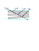
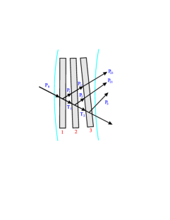
Figure 1: Crystal division in the Multilamellar model for a Bragg and Laue crystal with the respective transmitted and diffracted beams for Bragg (top) and Laue (bottom) geometries.

In the ML model it is assumed that the beam trajectory inside the crystal is a straight line. The crystal is perfect inside a given lamella, thus the crystal curvature cannot be large, otherwise it would originate local strains in the crystalline planes. The model is valid for crystals sufficiently thick to guarantee the existence of several lamellae. The model fails if the crystal thickness is of the order of or smaller than the lamella thickness. This may occur in Laue cases, where the crystal should be thin enough to guarantee a high transmission. The oscillations that may be found in Laue profiles calculated with the ML model are due to unphysical interferences between the crystal lamellae. A detailed description of the assumptions of this method is in [caciuffo_pr] and [chantler] and a good validation with experiments is in [Erola]

2.3 The Penning-Polder (PP) method

The PP theory is another geometrical approach widely used because of its simplicity in generating the beam trajectory inside the crystals. In the original model [PP01], only the two “normal wavefields” are accounted for. It is only valid when the disorientation of the crystal lattice planes over the Pendellösung length (or extinction length) is much smaller than the intrinsic reflection width of the perfect crystal. However, by including the two “created wavefields” from the interbranch scattering, the PP theory can be extended to the case of strongly distorted crystals [PP03, Schulze].

In the ray-optical theory of [PP01] the X-ray beam in a distorted crystal is assumed to be a pseudo-plane Bloch wave (”wavefield ray”) propagating parallel to the local Poynting vector. The crystal is supposed to be composed of parts of flat and undistorted crystals where the dynamical theory for perfect crystals can be applied. The wavefield is preserved passing from one part of the crystal to the next. Diffraction phenomena (the interference between two wavefields) are neglected. Thus, the Pendellösung fringes are not simulated with this model.

For crystals under constant strain gradient $\beta$ (see Appendix D) through the crystal thickness $T$, the ratio $\xi$ of the amplitudes of the diffracted and the transmitted waves can be obtained from Eq. 33 in [PP01]

$$2\eta=\xi_{e}-b/\xi_{e}=\xi_{i}-b/\xi_{i}+2\beta T,$$ (32)

where the subscript $e$ stands for the “exit” surface, $i$ denotes the “incident” surface.

The above equation generates two solutions for $\xi_{i}$ and another two for $\xi_{e}$:

$$\xi_{e,1}=\eta+\sqrt{\eta^{2}-b}$$

$$\xi_{e,2}=\eta-\sqrt{\eta^{2}-b}$$

$$\xi_{i,1}=\eta-\beta T+\sqrt{(\beta T-\eta)^{2}-b}$$ (33)

$$\xi_{i,2}=\eta-\beta T-\sqrt{(\beta T-\eta)^{2}-b}$$

these two solutions correspond to the splitting of the wavefields at the incident ($\xi_{i,j},j=1,2$) and exit surfaces ($\xi_{e,j}$). Most of the intensity goes along one mode for plane waves [PP03]. For each mode, the relationships between the intensity of the incident beam ($I_{0}$), the diffracted beam ($I_{R}$) and the transmitted beam ($I_{T}$) are (Eq. 35 in [PP01]):

$$\frac{I_{T,j}}{I_{0}}=\frac{b}{\xi_{i,j}^{2}+b}\frac{b}{\xi_{e,j}^{2}+b}\times$$

$$\exp\left\{-\frac{\mu T}{\gamma_{0}}\left[1+\frac{b-1}{2\beta T}(\xi_{e,j}-\xi_{i,j})+\frac{b}{\beta T}\frac{\mathfrak{Im}\sqrt{\Psi_{H}\Psi_{\bar{H}}}}{\mathfrak{Im}\Psi_{0}}\ln\frac{\xi_{e,j}}{\xi_{i,j}}\right]\right\},$$

$$\mathcal{R}_{j}=\frac{I_{R,j}}{I_{0}}=\frac{\xi_{e,j}^{2}}{b}\frac{I_{T,j}}{I_{0}}.$$ (34)

The total reflectivity $\mathcal{R}$ is then obtained by adding the intensities of the two $\xi$ solutions (one is usually very small), and removing the intensity of the created wavefields from the interbranch: scattering [PP03], or

$$\mathcal{R}=\mathcal{R}_{1}+\mathcal{R}_{2}=\left(\frac{I_{R,1}}{I_{o}}+\frac{I_{R,2}}{I_{o}}\right)\left[1-\exp\left(-\frac{2\pi\beta_{c}}{|\beta|}\right)\right],$$ (35)

where $\beta_{c}=\pi/(2\Lambda_{pend})$ is the critical strain gradient introduced by [Authier1970], with $\Lambda_{pend}$ the Pendellösung period as defined in Sec. 2.1. In case of overbending ($|\beta|>>\beta_{c}$), the $\mathcal{R}_{j}$ beams are attenuated and the intensity flows along the transmitted beam direction:

$$\mathcal{R}_{j}^{new}=\frac{I_{R,j}}{I_{o}}\exp\left(-\frac{2\pi\beta_{c}}{|\beta|}\right).$$ (36)

3 Examples of application

3.1 Cylindrically bent crystals in Bragg geometry

In a first example we checked the output of our code against the experimental case described in Fig. 4 of [Erola], where it is shown the reflectivity for symmetrical Si400 reflection using Mo K$\alpha_{1}$ radiation ($E=17479~{}eV$) for three bending radii: 1.1, 2.7 and 5.7 m. The bending is in the meridional plane, and the crystal is considered isotropic (Poisson’s ratio $\nu_{21}=-s_{21}/s_{22}=0.28$). The results of our simulations are in Fig. 2. The results including crystal anisotropy are almost identical to the isotropic case.

\begin{overpic}[width=252.94499pt]{fig_erola.eps} \put(50.0,15.0){\includegraphics[width=108.405pt]{fig_erola_inset.eps}} \end{overpic}

Figure 2: Calculated reflectivity curves for an isotropic symmetrical Si400 crystal reflection at photon energy $E=17479~{}eV$ ($\sigma$-polarized) for three curvature radii: $R=5.7~{}m$ (solid line), $R=2.7~{}m$ (dashed line) and $R=1.1~{}m$. The inset displays a sketch of the geometry. Results are in agreement with [Erola].

3.2 Laue cylindrically bent crystal in meridional plane

We calculate here the case described in [Schulze] and treated extensively in [SchulzeThesis]. It consists of a Si111 crystal of thickness $T=700~{}\mu m$ diffracting at $E=33170~{}eV$, bent with meridional Radius $R=325~{}cm$ (convex to the beam). The crystal directions for $\alpha_{X}=0$ are $\vec{n}=1~{}1~{}1$, $\vec{v}_{along}=\bar{1}~{}1~{}0$, and $\vec{v}_{\perp}=1~{}1~{}\bar{2}$. The asymmetrical cut is $\alpha_{X}=296.2^{\circ}$ ($\alpha=-116.2^{\circ}$, $\chi=-206.2^{\circ}$). As discussed by Schulze, the anisotropy in the crystal is an important factor to be considered. Figure 3 illustrates this by comparing the calculated diffraction profiles for three cases: i) the isotropic crystal, ii) the original crystal configuration (with $\vec{v}_{\perp}=1~{}1~{}\bar{2}$), and iii) another crystal cut ($\vec{v}_{\perp}=1~{}\bar{1}~{}0$). It can be shown here that the curves generated by the two methods are in quite good agreement. Fig. 4 shows the variation of the diffraction profile as a function of the bending radius.

\begin{overpic}[width=252.94499pt]{fig_clemens_comparison_iso.eps} \put(185.0,35.0){\includegraphics[width=72.26999pt]{diff_pat_bent_clemens.eps}} \end{overpic}

Figure 3: Diffraction profiles for a meridionally bent ($R$=325 cm), $T=700~{}\mu m$ thick silicon crystal at $E=33170~{}eV$. The calculations show the results for the asymmetric ($\alpha_{X}=296.2^{\circ}$) 111 reflection for the isotropic crystal (green lines, $\nu=0.274$) and two different crystal cuts: i) $\vec{v}_{\perp}=1~{}1~{}\bar{2}$ (red lines) and ii) $\vec{v}_{\perp}=1~{}\bar{1}~{}0$ (blue lines). The solid lines have been calculated using the Penning-Polder model and the dashed lines used the multilamellar model. In this case, 1$\eta=3.87\mu rad$. The inset displays a sketch of the geometry.

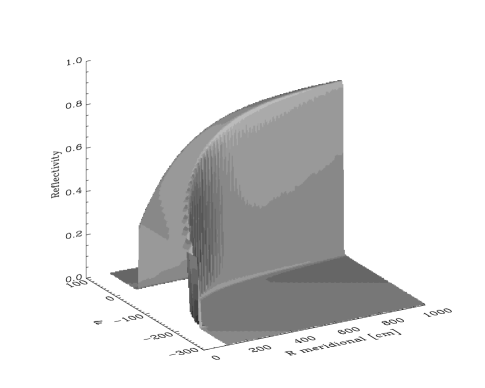
Figure 4: Diffraction profiles computed using the Penning-Polder model for a crystal with parameters like in Fig. 3 ($\vec{v}_{\perp}=1~{}1~{}\bar{2}$) as a function of the bending radius.

The compliance tensor for the chosen crystal cut and asymmetry angle is shown in Table 1. The variation of the components of the compliance tensor versus asymmetry angle that affect the diffraction profile are in Fig. 5.

Table 1: Compliance tensor values ($\times 10^{-12}~{}m^{2}/N$) for an asymmetric ($\alpha_{X}=296.2^{\circ}$) silicon 111 crystal. In bold the elements that affect the $\beta$ and $c$ parameters for pure meridional bending. The underlined elements contribute to the anticlastic bending.

$j$	$s_{1j}$	$s_{2j}$	$s_{3j}$	$s_{4j}$	$s_{5j}$	$s_{6j}$
1	5.920	-1.081	-1.439	-0.465	-0.733	1.489
2	-1.081	6.092	-1.611	1.225	-1.037	-0.871
3	-1.439	-1.611	6.450	-0.760	1.769	-0.618
4	-0.465	1.225	-0.760	14.715	-1.236	-2.074
5	-0.733	-1.037	1.769	-1.236	15.404	-0.930
6	1.489	-0.871	-0.618	-2.074	-0.930	16.836

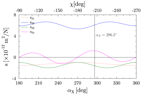
Figure 5: Variation of the elements of the compliance tensor that affect diffraction for meridional bending versus asymmetry angle $\alpha_{X}$ or $\chi$. Continuous lines: elements affecting $c$ and $\beta$. Dotted line: element affecting anticlastic bending.

3.3 Optimization of a Laue cylindrically bent crystal in meridional plane

We calculate here the diffraction profile for Laue crystals to be used by the high energy X-ray monochromator proposed for the Upgrade ESRF beamline ID31 (UPBL02) [UPBL02]. The monochromator holds two bent Laue crystals for monochromatizing the beam in the photon energy range 50-150 keV with variable energy resolution in the range $\Delta E/E\approx 10^{-4}-10^{-2}$. controlled by the crystal bending. The diffraction plane is horizontal. We simulate a single silicon crystal at energy $E=70~{}keV$ using either the reflections 111 (for low energy and low resolution) or 113 (for high resolution and high energy applications). The crystals parameters are in Table 2. Fig. 6 shows the resulting diffraction profile for the 111 reflection and Fig. 7 considered crystal configuration.

Table 2: Inputs for a meridionally bent crystal.$R=10530cm/\gamma_{0}$

Crystal	Si 111	Si 311
Photon energy	70 keV
Crystal thickness	0.5 cm
Meridional Radius (convex to the beam)	12759 cm	10551 cm
Asymmetry $\alpha_{X}$	$234^{\circ}$	$263.5^{\circ}$
Asymmetry $\chi$	$-144^{\circ}$	$-173.5^{\circ}$
Crystal cut (for $\alpha_{X}=0$)	$\vec{n}=1~{}1~{}1$ $\vec{v}_{along}=\bar{1}~{}\bar{1}~{}2$ $\vec{v}_{\perp}=\bar{1}~{}1~{}0$	$\vec{n}=1~{}1~{}3$ $\vec{v}_{along}=\bar{3}~{}\bar{3}~{}2$ $\vec{v}_{\perp}=\bar{1}~{}1~{}0$

\begin{overpic}[width=252.94499pt]{fig_veijo111.eps} \put(175.0,50.0){\includegraphics[width=90.3375pt]{diff_pat_bent_veijo111.eps}} \end{overpic}

Figure 6: Diffraction profile for the Si111 crystal with parameters in Table 2.

\begin{overpic}[width=252.94499pt]{fig_veijo113.eps} \put(50.0,50.0){\includegraphics[width=90.3375pt]{diff_pat_bent_veijo113.eps}} \end{overpic}

Figure 7: Diffraction profile for the Si113 crystal with parameters in Table 2.

The crystal has been optimized in the following way: i) the crystal cut is chosen in such a way that $\vec{v}_{\perp}=\bar{1}~{}1~{}0$ so the compliance coefficient $s_{61}$ and $s_{62}$ are zero for any asymmetry angle. Therefore, the crystal is not twisted thus keeping $\vec{k}^{0}$, $\vec{k}^{H}$and $\vec{H}$ in the 23 plane. The crystal is cut with an asymmetry angle that on one side permits to use both Si111 and Si113 for low and high resolution applications, respectively; and on the other side is optimized for giving good integrated reflectivity. Fig. 8 shows the integrated reflectivity and energy bandwidth as a function of asymmetry angle and thickness, with indication of the selected working points.

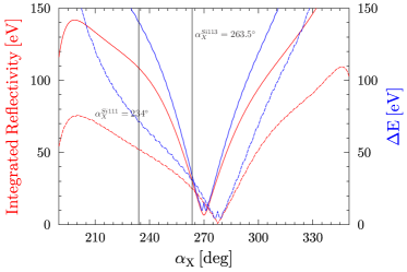
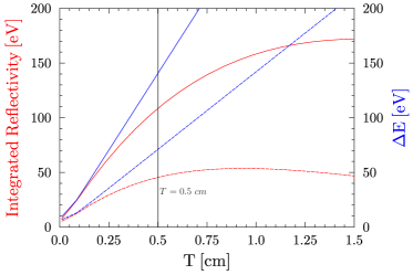
Figure 8: Left: Dependency of integrated reflectivity (red) and $\Delta E$ (blue) for Si111 (solid) and Si113 (dotted) as a function of the asymmetry angle $\alpha_{X}$ (left). Right: Variation of integrated reflectivity (red) and $\Delta E$ (blue) for Si111 at 70 keV (solid) and 50 keV (dotted) as a function of crystal thickness (right).

The same physical crystal should be used for 111 and 113 reflections, and its compliance tensor is shown in Table 3. The variation as a function of the asymmetry (measured for Si111) of the components contributing to the diffraction is in Fig. 9.

Table 3: Compliance tensor values ($\times 10^{-12}~{}m^{2}/N$) for an asymmetric ($\alpha_{X}=234^{\circ}$) Si111 crystal (or $\alpha_{X}=263.5^{\circ}$ Si113, corresponding to the same crystal cut). In bold the elements that affect the $\beta$ and $c$ parameters for pure meridional bending. The underlined elements contribute to the anticlastic bending.

$j$	$s_{1j}$	$s_{2j}$	$s_{3j}$	$s_{4j}$	$s_{5j}$	$s_{6j}$
1	5.920	-1.958	-0.562	1.071	0.000	0.000
2	-1.958	7.010	-1.651	-1.810	0.000	0.000
3	-0.562	-1.651	5.613	0.739	0.000	0.000
4	1.071	-1.810	0.739	14.554	0.000	0.000
5	0.000	0.000	0.000	0.000	18.914	2.141
6	0.000	0.000	0.000	0.000	2.141	13.326

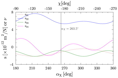
Figure 9: Variation of the elements of the compliance tensor that affect diffraction for meridional bending versus asymmetry angle $\alpha_{X}$ or $\chi$ for Si111. Continuous lines: elements affecting $c$ and $\beta$. Dotted line: element affecting anticlastic bending.

3.4 Laue cylindrically bent crystal in sagittal plane

In this section we analyze a Si$\bar{1}\bar{1}\bar{1}$ crystal 0.07 cm thick used to focus a 50 keV X-ray beam in sagittal direction [xianbo_spie]. The diffraction plane in the meridional direction is affected by the anticlastic curvature originated by the sagittal radius, which is much smaller that the typical radii used in meridional focusing. One of the main roles of the crystal is to focus the beam in the sagittal direction, and to match the beam divergence in the meridional direction (Rowland condition). The optimized meridional radius $R_{m}$ is normally more than ten times larger than the sagittal radius $R_{s}$ required for focusing (e.g., in [ShiJSR]). Therefore, in most cases the Poisson’s ratio $\nu$ must be minimized ($R_{m}=R_{s}/\nu$, with, $R_{s}=R_{1}$ the sagittal radius and $\nu=-s_{12}/s_{11}$). Fig. 10 shows the variation of the Poisson’s ratio for different crystal cuts. From this graphic it is selected the crystal cut ($\vec{n}=\bar{1}~{}\bar{1}~{}\bar{1}$, $\vec{v}_{along}=\bar{2}~{}1~{}1$, and $\vec{v}_{perp}=0~{}\bar{1}~{}1$ ) and asymmetry ($\alpha_{X}=125.26^{\circ}$ or $\chi=-35.26^{\circ}$). The compliance tensor is shown in Table 4. Fig. 11 shows the diffraction profile.

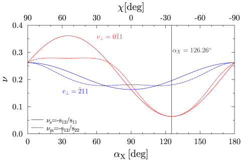
Figure 10: Variation of Poisson’s ratio versus asymmetry angle $\alpha_{X}$ (deg)

\begin{overpic}[width=252.94499pt]{fig_xianbo.eps} \put(40.0,50.0){\includegraphics[width=90.3375pt]{diff_pat_bent_xianbo.eps}} \end{overpic}

Figure 11: Diffraction profiles for a sagittaly bent Si$\bar{1}\bar{1}\bar{1}$ crystal (see text) calculated using the Penning-Polder (red) and multilamellar (blue) models. In this case, $1\eta=2.57~{}\mu rad$.

Table 4: Compliance tensor values ($\times 10^{-12}~{}m^{2}/N$) for asymmetric ($\alpha_{X}=125.26^{\circ}$) Si$\bar{1}\bar{1}\bar{1}$ crystal. In bold the elements that affect the $\beta$ and $c$ parameters for pure meridional bending. The underlined elements contribute to the anticlastic bending.

$j$	$s_{1j}$	$s_{2j}$	$s_{3j}$	$s_{4j}$	$s_{5j}$	$s_{6j}$
1	5.920	-0.380	-2.140	0.000	0.000	0.000
2	-0.380	5.920	-2.140	-0.000	0.000	0.000
3	-2.140	-2.140	7.680	0.000	0.000	0.000
4	0.000	0.000	0.000	12.600	0.000	0.000
5	0.000	0.000	0.000	0.000	12.600	0.000
6	0.000	0.000	0.000	0.000	-0.000	19.640

4 Discussion and conclusions

In the last section several diffraction profiles corresponding to Bragg and Laue geometries are considered. Numerical calculations have provided the diffraction profiles. It is possible in some cases to obtain some physical parameters like the width of the reflections, energy resolution and integrated intensities from simple analytical expressions obtained from the approximated methods applied. Some of these results are discussed in this paragraph.

For Bragg curved crystals the multilamellar is the only method that can be applied among the ones described here. The shape of the diffraction profile is approximately triangular in the case of ”thick“ crystals. The integrated reflectivity $R_{\eta}$ increases with curvature (inverse of radius). The integrated intensity (as a function of the $\eta$ variable) varies from $R_{\eta}=\pi$ for the non-absorbing thick crystal ($R_{\eta}=8/3$ for the Darwin solution) to the kinematical limit $R_{\eta}^{K}=\pi^{2}|\Psi_{H}|/(2\lambda\mu)$ (mosaic crystals). For instance, for the Si400 calculated in Fig. 2 $R_{\eta}^{K}=85.47$ and $R_{\eta}=20.66,36.44,57.47$ for radii $R=5.7,2.7,1.1~{}m$ (number of lamellae $1074,2269,5570$), respectively. In case of thin crystals, the diffraction profile does not decrease asymptotically to zero but decreases abruptly when at a given angle related to the crystal thickness. It produces a trapezoidal-shaped profile for Bragg crystals, and an almost rectangular shape for Laue crystals (as seen in all Laue examples discussed in last section). The width of the reflection is (from Eq. 2.2) $\Delta\eta=cA=cT\Lambda/2$. The energy bandwidth is calculated using the derivative of the Bragg law and Eq. 23:

$$\frac{\Delta\lambda}{\lambda}=-\frac{\Delta E}{E}=\cot\theta_{B}\Delta\theta=\frac{\pi P^{2}|\Psi_{H}|^{2}}{2\lambda|\gamma_{0}|\sin^{2}\theta_{B}}cT$$ (37)

Results of values given by Eq. 37 to the Laue crystals discussed in the last section are shown in Table 5.

For Laue crystals the PP method gives a diffraction profile width $\Delta\eta\approx\beta T$ in case of low-absorbing crystals curved enough to produce a diffraction width much larger than the perfect (undistorted) crystal ($\Delta\eta\gg 2$). Using Eq. D it gives a bandwidth of:

$$\frac{\Delta\lambda}{\lambda}=-\frac{\Delta E}{E}=\frac{GT}{2k^{0}\gamma_{0}\sin^{2}\theta_{B}}$$ (38)

Table 5: Comparison of energy bandwidth for different Laue crystal reflections analyzed in previous section.

	Fig. 3	Fig. 6	Fig. 7	Fig. 11
$\Delta E$ FWHM from ML profile	142.9	138.0	30.6	64.8
$\Delta E$ Eq. 37	142.5	141.6	31.3	68.8
$\Delta E$ FWHM from PP profile	143.5	140.6	30.9	69.0
$\Delta E$ Eq. 38	143.5	141.3	31.1	68.8

The numerical values for energy bandwidth given by the analytical formulas agree very well with the calculated ones. In fact, both models agree if $\beta T=cA$ which implies that

$$\frac{d\alpha_{Z}}{dt}=\frac{1}{\gamma_{0}k^{0}}\frac{\partial^{2}(\vec{H}.\vec{u})}{\partial V_{0}\partial V_{H}}$$ (39)

Therefore, both models are consistent in giving the same $\Delta E$, they give approximated peak reflectivities (checked numerically for the treated cases), but will produce different ray trajectories (not discussed here).

We compare now the diffraction profiles produced by the same crystal curved along the sagittal direction with the same crystal curved with the same radius $R=$-125 cm along the meridional direction, or in both direction (spherical). The results are shown in Fig. 12 showing remarkable differences. The broadening of the diffraction profile is produced by the curvature in the diffraction plane, therefore the broadening is very important for pure meridional or spherical bending. For sagittal bending, the broadening is much smaller, because the curvature in the meridional plane is due to the larger anticlastic radius $R_{anticlastic}=-R_{m}/\nu_{s}$, where $R_{m}$ is the meridional bending and $\nu_{s}=-s_{12}/s_{11}=0.064$ is the Poisson’s ratio in sagittal direction. In fact, the diffraction profile calculation for sagittally bent crystal of $R=-125~{}cm$ is very well approximated by a meridional bending with $R_{anticlastic}=1947.37~{}cm$ (see Fig. 12).

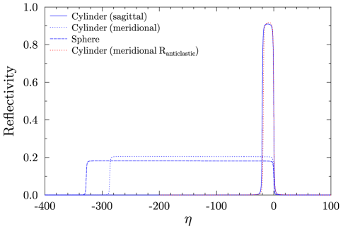
Figure 12: Comparison of the reflectivity curve for the crystal in Fig. 11 (pure sagittal bending, $R_{s}=-125~{}cm$ solid line), with the pure meridional bending ($R_{m}=-125~{}cm$, dotted line), and spherical bending ($R_{s}=R_{m}=-125~{}cm$ dashed line). In red, the diffraction profile produced by a crystal bent in the meridional direction with $R_{anticlastic}=1947.37~{}cm$.

This paper concerns distorted crystals in which the deformation is created by bending the crystal, usually elastic bending. In most cases the crystal curvature is created with the aim of focusing or collimating the X-ray beam, usually in the meridional plane, but sometimes in the sagittal direction. We discussed the general case of curvature in both directions, which is of interest for spherical bending (equal two-moments), toroidal (different two-moments), or when cylindrical bending is requested (one-moment bending). In this last case, however, the elastic properties of the materials induce the anticlastic curvature in the perpendicular direction. Another important source of deformation for crystals in synchrotron beamlines is the thermal load. Although a full analysis of the crystal reflectivity for heat load in crystals is out of the scope of this paper, the same approximated methods to calculate the diffraction profiles can be used. In fact, the original work of [Penning] also gives the value of $\beta$ for a crystal deformed by a uniform temperature gradient. Also, our code can be used to estimate if the thermal deformation affects the diffraction properties of the crystal by calculating the diffraction profiles for a curvature radius $R$ due to the thermal bending of the crystal [Kalus1973]:

$$R=\frac{T}{\Delta_{T}\alpha_{S}}$$ (40)

where $T$ is the crystal thickness, $\alpha_{S}$ is the thermal expansion coefficient of the crystal and $\Delta_{T}$ is the temperature difference between the two faces of the crystal that is approximately proportional to the absorber power $\Delta_{T}=PT/\kappa$, with $\kappa$ the diffusion coefficient. This only gives a first estimation of the possible alteration of the diffraction profile. Other effects must be considered, like the thermal expansion of the crystal unit cell, and the changes in the rocking curves because of the reflection in a non-planar crystal surface [ZhangMonochromators].

In conclusion, we summarized the formulation of two approximated methods for calculating diffraction profiles: the multilamellar applied for both Bragg and Laue bent crystals, and the Penning-Polder only applicable to Laue crystals. We obtained the general expression of the constant strain parameter ($\beta$ for PP and $c$ for ML) including crystal anisotropy for any asymmetric crystal cut. The general expressions obtained reduce to the formulations of particular cases from literature. Last, some approximated expressions for obtaining the angular and energy bandwidths of these crystals are given.

The equations are implemented in the XOP package and are validated by studying some examples analyzed in literature. The XOP user has access to these calculations using the usual XCRYSTAL application. The input files for XCRYSTAL with the input parameters of the cases studied in this paper are available in the examples directory of the XOP distribution. The code is also provided in open source under the GPL license at https://github.com/srio/CRYSTAL.

Appendix A Geometry, scattering vectors and angles

We define an orthonormal reference frame intrinsic to the crystal with origin at the crystal center (usually where the central ray intercept the crystal) and three vectors $(\vec{n},\vec{v}_{along},\vec{v}_{\perp})$, being $\vec{n}$ a unity vector normal to the crystal surface pointing outside the crystal bulk, and $\vec{v}_{along}$ and $\vec{v}_{\perp}$ two orthonormal vectors in the plane of the crystal surface, usually chosen to be inside and perpendicular to the diffraction plane, respectively. A crystal cut is defined by the asymmetry angle, either $\alpha$ or $\chi$. Usually $\alpha$ is used in Bragg geometry and $\chi$ in Laue geometry, but if both values are well-defined they can be used indistinctly in both geometries.

For the formulas used in this text, implemented in the XOP code, we have used the following definitions and conventions:

• For simplicity, the three reference vectors previously defined match a simple laboratory reference system chosen $\vec{n}=(0,0,1)$, $\vec{v}_{along}=(0,1,0)$ and $\vec{v}_{\perp}=(1,0,0)$. The normal of the reflecting crystal surface $\vec{n}$ is pointing outside from the crystal. A generic point in the crystal has as coordinates $\vec{r}=(x_{1},x_{2},x_{3})$.

• We define $\chi$ as the angle from $x_{2}$ axis to $\vec{H}$ (in mathematical sense, positive if counterclockwise (ccw)). The angle $\alpha=\chi+90^{\circ}$ goes from the crystal surface to the the Bragg planes $hkl$ (measured from $x_{2}$ axis to the reflecting surface, thus for symmetric Bragg case $\alpha=180^{\circ}$). The asymmetry angle $\alpha_{X}$ defined in XOP (from crystal surface to crystal planes, positive if clockwise (cw)) holds $\alpha_{X}+\alpha=180^{\circ}$. See Fig. 13.

• The reciprocal lattice vector $\vec{H}$ can be obtained by rotating the normal to the surface $\vec{n}$ an angle $\theta=\chi-90^{\circ}=-\alpha_{X}$ around the vector $\vec{v}_{\perp}$: $\vec{H}=ROT_{\vec{v}_{\perp}}(\vec{n},\theta)$. The $ROT$ operator is implemented via the Rodrigues formula that rotates a vector $\vec{V}$ an angle $\theta$ around an axis $\vec{a}$ (normalized, $\theta$ is positive in the screw (cw) sense when looking in the direction of $\vec{a}$) to obtain $\vec{V_{rot}}$:

  $$\vec{V}_{rot}=ROT_{\vec{a}}(\vec{V},\theta)=\vec{V}\cos\theta+$$

  $$(\vec{a}\times\vec{V})\sin\theta+\vec{a}~{}(\vec{a}\cdot\vec{V})(1-\cos\theta).$$ (A.1)

• The (unsigned) Bragg angle verifies $\lambda=2d_{hkl}\sin\theta_{B}$, with $\lambda$ the photon wavelength in vacuum. The direction of an incident beam that fulfils Bragg’s law makes an angle $\theta_{B}$ with respect to the Bragg planes, therefore its direction is: $\vec{V}^{0}_{B}=ROT_{\vec{v}_{\perp}}(-\vec{H},90^{\circ}-\theta_{B})$.

The diffraction profile for a given hkl reflection is obtained by scanning the direction $\vec{V}^{0}$ of a monochromatic collimated incident beam (a plane wave) in the vicinity of $\vec{V}^{0}_{B}$ in the diffraction plane. If both vectors are separated by an angle $\Delta\theta=|\theta|-|\theta_{B}|$ we can set $\vec{V}^{0}=ROT_{\vec{v}_{\perp}}(\vec{V}^{0}_{B},-\Delta\theta)$.

The vector expressions can be expressed in angles, but care must be taken with the definition and sign of angles.

The incident angle (measured ccw from $x_{2}$ to $\vec{V}^{0}$) for the ray fulfilling the Bragg law (in both Bragg and Laue geometries) is $\theta_{0}=180^{\circ}+\alpha-\theta_{B}$, and the reflected angle (measured ccw from $x_{2}$ to $\vec{V}^{H}$) is $\theta_{H}=180^{\circ}+\alpha-\theta_{B}$. In Laue geometry, for a given crystal cut, we may send the beam to match the Bragg angle below or onto the Bragg planes (which strictly speaking correspond to using $\pm\vec{H}$), and reversing time. From these four cases only two are independent.

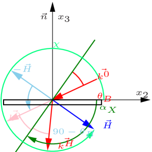
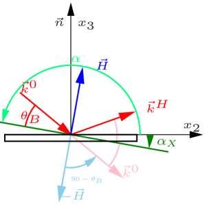
Figure 13: Schematic view of diffraction using asymmetric Si111 crystals at $E=4~{}keV,~{}\theta_{B}=29.62^{\circ}$. Left: Laue geometry: $\alpha_{X}=125.26^{\circ},\chi=-35.26^{\circ},~{}\alpha=54.74^{\circ}$. Right: Bragg geometry: $\alpha_{X}=10^{\circ},\chi=80^{\circ},~{}\alpha=170^{\circ}$. The plotted incident direction corresponds to the Bragg position $\vec{V}^{0}_{B}$, so here $\vec{k^{0}}=\vec{k^{0}_{B}}$.

The directions (as as function of $\alpha$, $\alpha_{X}=180^{\circ}-\alpha$, and $\chi=\alpha-90^{\circ}$), for the directions fulfilling the Bragg law (Eq. 1) are:

$$\vec{V}^{0}_{B}=(0,\cos\theta_{0},\sin\theta_{0})=$$

$$(0,-\cos(\theta_{B}-\alpha),\sin(\theta_{B}-\alpha))=$$

$$(0,\cos(\theta_{B}+\alpha_{X}),-\sin(\theta_{B}+\alpha_{X}))=$$

$$(0,-\sin(\theta_{B}-\chi),-\cos(\theta_{B}-\chi))$$

$$\vec{V}^{H}_{B}=(0,\cos\theta_{H},\sin\theta_{H})=$$

$$(0,-\cos(\theta_{B}+\alpha),-\sin(\theta_{B}+\alpha))=$$ (A.2)

$$(0,\cos(\theta_{B}-\alpha_{X}),\sin(\theta_{B}-\alpha_{X}))=$$

$$(0,\sin(\theta_{B}+\chi),-\cos(\theta_{B}+\chi))$$

$$\vec{n}^{H}=(0,\sin\alpha,-\cos\alpha)=$$

$$(0,\sin\alpha_{X},\cos\alpha_{X})=$$

$$(0,\cos\chi,\sin\chi)$$

Appendix B Elastically bent crystals

B.1 Bending an anisotropic plate

The generalized Hooke’s law makes a “linear” relation between the the $strain$ tensor ($S^{\prime}_{ij}$, $i,j=1,2,3$, characterizing the deformation, adimensional), and the $stress$ tensor ($\sigma^{\prime}_{kl}$, $k,l=1,2,3$, generalized forces with dimension of force times $L^{-2}$) (Eq. 1.3.2 in [hearmon]):

$$S^{\prime}_{ij}=s^{\prime}_{ijkl}\sigma^{\prime}_{kl}$$ (B.1)

where $s^{\prime}_{ijkl}$ is the $elastic~{}compliance$ tensor. The stiffness tensor is the inverse of the compliance tensor, but here we will center the discussion on the compliance tensor only. Each index can take three values (1,2,3, corresponding to the three directions in 3D space) and the repeated indices are summed. From symmetry considerations, not all 81 elements of the compliance are independent, but they are reduced to 36. Moreover, thermodynamical considerations reduce the number of independent compliance elements to a maximum of 21 in the most general case. These facts make possible to reduce Eq. (B.1) to a simpler form (Eq. 1.3.6 in [hearmon]):

$$S_{q}=s_{qr}\sigma_{r}~{}~{}(q,r=1,...,6),$$ (B.2)

with now $s_{qr}$ a 36 elements symmetric matrix. The new strain 6-dim vector as a function of the old strain tensor is (Eq. 1.2.8 in [hearmon]):

$$S_{1}=S^{\prime}_{11},~{}S_{2}=S^{\prime}_{22},~{}S_{3}=S^{\prime}_{33},$$

$$~{}S_{4}=2S^{\prime}_{23},~{}S_{5}=2S^{\prime}_{13},~{}S_{6}=2S^{\prime}_{12},$$ (B.3)

(the same convention applies for indices from $s^{\prime}$ to $s$, e.g., $s_{36}=s^{\prime}_{3312}$), and (Eq. 1.2.4 in [hearmon])

$$S^{\prime}_{i,j}=\frac{1}{2}\left(\frac{\partial u_{i}}{\partial x_{j}}+\frac{\partial u_{j}}{\partial x_{i}}\right)$$ (B.4)

with $u_{i}$ the displacements (elongations) and $x_{i}$ the coordinates along the three spatial dimensions $i=1,2,3$.

Then, Eq. B.2 can be expanded as:

$$\frac{\partial u_{1}}{\partial x_{1}}=s_{11}\sigma^{\prime}_{11}+s_{12}\sigma^{\prime}_{22}+s_{13}\sigma^{\prime}_{33}+s_{14}\sigma^{\prime}_{23}+s_{15}\sigma^{\prime}_{13}+s_{16}\sigma^{\prime}_{12}$$

$$\frac{\partial u_{2}}{\partial x_{2}}=s_{21}\sigma^{\prime}_{11}+s_{22}\sigma^{\prime}_{22}+s_{23}\sigma^{\prime}_{33}+s_{24}\sigma^{\prime}_{23}+s_{25}\sigma^{\prime}_{13}+s_{26}\sigma^{\prime}_{12}$$

$$\frac{\partial u_{3}}{\partial x_{3}}=s_{31}\sigma^{\prime}_{11}+s_{32}\sigma^{\prime}_{22}+s_{33}\sigma^{\prime}_{33}+s_{34}\sigma^{\prime}_{23}+s_{35}\sigma^{\prime}_{13}+s_{36}\sigma^{\prime}_{12}$$

$$\frac{\partial u_{2}}{\partial x_{3}}+\frac{\partial u_{3}}{\partial x_{2}}=s_{41}\sigma^{\prime}_{11}+s_{42}\sigma^{\prime}_{22}+s_{43}\sigma^{\prime}_{33}+s_{44}\sigma^{\prime}_{23}+s_{45}\sigma^{\prime}_{13}+s_{46}\sigma^{\prime}_{12}$$ (B.5)

$$\frac{\partial u_{1}}{\partial x_{3}}+\frac{\partial u_{3}}{\partial x_{1}}=s_{51}\sigma^{\prime}_{11}+s_{52}\sigma^{\prime}_{22}+s_{53}\sigma^{\prime}_{33}+s_{54}\sigma^{\prime}_{23}+s_{55}\sigma^{\prime}_{13}+s_{56}\sigma^{\prime}_{12}$$

$$\frac{\partial u_{1}}{\partial x_{2}}+\frac{\partial u_{2}}{\partial x_{1}}=s_{61}\sigma^{\prime}_{11}+s_{62}\sigma^{\prime}_{22}+s_{63}\sigma^{\prime}_{33}+s_{64}\sigma^{\prime}_{23}+s_{65}\sigma^{\prime}_{13}+s_{66}\sigma^{\prime}_{12}$$

In general, the stress tensor is proportional to the generalized torques $M$ (per unit of length) and forces $A$. Let us suppose a crystal as a rectangular plate of thickness $T$ with axes 1 and 2 parallel to the the edges, and axis 3 perpendicular to the surface. Considering only two torques $M_{1}$ and $M_{2}$ (dimensions torque per length), applied in-plane (Fig. 14), we have:

$$\sigma^{\prime}_{11}=\frac{M_{1}x_{3}}{I}$$

$$\sigma^{\prime}_{22}=\frac{M_{2}x_{3}}{I}$$

$$\sigma^{\prime}_{33}=0$$ (B.6)

$$\sigma^{\prime}_{13}=\sigma^{\prime}_{23}=\sigma^{\prime}_{12}=0$$

where the zero terms are a consequence of considering pure bending, and $I=T^{3}/12$ is the inertia moment.

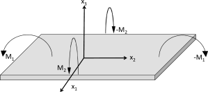
Figure 14: Double moment bending of a rectangular plate of thickness $T$

Replacing all $\sigma^{\prime}_{ij}$ into Eq. (B.1) we obtain:

$$\frac{\partial u_{1}}{\partial x_{1}}=\frac{1}{I}\left(s_{11}M_{1}x_{3}+s_{12}M_{2}x_{3}\right)$$

$$\frac{\partial u_{2}}{\partial x_{2}}=\frac{1}{I}\left(s_{21}M_{1}x_{3}+s_{22}M_{2}x_{3}\right)$$

$$\frac{\partial u_{3}}{\partial x_{3}}=\frac{1}{I}\left(s_{31}M_{1}x_{3}+s_{32}M_{2}x_{3}\right)$$ (B.7)

$$\frac{\partial u_{2}}{\partial x_{3}}+\frac{\partial u_{3}}{\partial x_{2}}=\frac{1}{I}\left(s_{41}M_{1}x_{3}+s_{42}M_{2}x_{3}\right)$$

$$\frac{\partial u_{1}}{\partial x_{3}}+\frac{\partial u_{3}}{\partial x_{1}}=\frac{1}{I}\left(s_{51}M_{1}x_{3}+s_{52}M_{2}x_{3}\right)$$

$$\frac{\partial u_{1}}{\partial x_{2}}+\frac{\partial u_{2}}{\partial x_{1}}=\frac{1}{I}\left(s_{61}M_{1}x_{3}+s_{62}M_{2}x_{3}\right)$$

Integrating these equation we obtain (Eq. 4 in [chukhovskii1992]):

$$u_{1}=\frac{1}{I}[(s_{11}M_{1}+s_{12}M_{2})x_{1}x_{3}$$

$$+(s_{51}M_{1}+s_{52}M_{2})x_{3}^{2}/2+(s_{61}M_{1}+s_{62}M_{2})x_{2}x_{3}/2]$$

$$u_{2}=\frac{1}{I}[(s_{21}M_{1}+s_{22}M_{2})x_{2}x_{3}$$

$$+(s_{41}M_{1}+s_{42}M_{2})x_{3}^{2}/2+(s_{61}M_{1}+s_{62}M_{2})x_{1}x_{3}/2]$$ (B.8)

$$u_{3}=\frac{1}{2I}[-(s_{11}M_{1}+s_{12}M_{2})x_{1}^{2}-(s_{21}M_{1}+s_{22}M_{2})x_{2}^{2}$$

$$-(s_{61}M_{1}+s_{62}M_{2})x_{1}x_{2}+(s_{31}M_{1}+s_{32}M_{2})x_{3}^{2}]$$

Replacing $x_{3}=-T/2$ we obtain the equation of the plate surface (Eq. 5a in [chukhovskii1992])):

$$u_{3}=-(s_{11}M_{1}+s_{12}M_{2})\frac{x_{1}^{2}}{2I}-(s_{21}M_{1}+s_{22}M_{2})\frac{x_{2}^{2}}{2I}$$

$$-(s_{61}M_{1}+s_{62}M_{2})\frac{x_{1}x_{2}}{2I}+(s_{31}M_{1}+s_{32}M_{2})\frac{T^{2}}{8I}$$ (B.9)

From here, one can obtain the profiles along the $i=1,2$ directions, which are approximately circular with the form $u_{3}=-x_{i}^{2}/(2R_{i})$. The radii are: (Eq. 5b in [chukhovskii1992])):

$$\frac{1}{R_{1}}=s_{11}\frac{M_{1}}{I}+s_{12}\frac{M_{2}}{I}$$

$$\frac{1}{R_{2}}=s_{21}\frac{M_{1}}{I}+s_{22}\frac{M_{2}}{I}$$ (B.10)

From Eq. (B.10) is possible to calculate the applied torques as a function of the curvatures:

$$\frac{M_{1}}{I}=\frac{1}{s_{12}s_{21}-s_{11}s_{22}}\left(\frac{s_{12}}{R_{2}}-\frac{s_{22}}{R_{1}}\right)$$ (B.11)

$$\frac{M_{2}}{I}=\frac{1}{s_{12}s_{21}-s_{11}s_{22}}\left(\frac{s_{21}}{R_{1}}-\frac{s_{11}}{R_{2}}\right)$$

The Eq. B.8 give the displacements $u_{i}$ knowing the elastic compliance tensor and the torques applied (or more interestingly, via the bending radii using Eq. B.10).

B.2 The compliance tensor for crystals cut along given directions

The number of independent components in the compliance tensor depends on the crystal symmetry. For a crystal cut along the crystallographic axes, triclinic crystals have all 21 components independent, monoclinic crystals have 13, orthorhombic crystal 9, tetragonal crystals 6 or 7 and cubic crystals 3 (see table 5 in [hearmon]). An isotropic material has only two independent components. For a crystal cut along given directions, fourth-rank compliance tensor must be transformed following (Eq. 1.5.2 in [hearmon]):

$$s^{{}^{\prime\prime}}_{ijkl}=a_{im}a_{jn}a_{ko}a_{lp}s^{\prime}_{mnop}$$ (B.12)

where the elements of the $a$ tensor are the direction cosines of the new axes. Software codes are available [VeijoPC] [Schulze] to transform a generic compliance tensor expressed in the reference frame coincident with the crystallographic axes, to a new one where the crystal has been cut following known planes expressed by their Miller indices.

For a cubic crystal cut along its crystallographic axes, the compliance tensor has only three different values. The non-zero elements are: $s_{12}=s_{21}=s_{13}=s_{31}=s_{23}=s_{32}$, $s_{11}=s_{22}=s_{33}$ and $s_{44}=s_{55}=s_{66}$. Because of cubic symmetry, this tensor is independent on the choice of the axes in the crystal (in plane or normal). The components of the compliance tensor for the most usual crystals are expressed in Table 6. The components of the compliance tensor for a cubic crystal cut along a given direction can be calculated using the generic Eq. (B.12), resulting in analytical expressions given by [wortman]. A convenient form easy to implement in computer languages is given in [linzhang] [zhangJSR] .

In the particular case of one single torque ($M_{2}=0$) Eqs. (B.10) give the main bending radius $R_{1}=I/(s_{11}M_{1})$ and a curvature radius in the perpendicular direction $R_{2}=R_{1}(s_{11}/s_{12})$, the anticlastic curvature. The ratio of the transverse component of the compliance tensor (in this case along the direction $12$) over the longitudinal component is the Poisson’s ratio $\nu_{12}=-s_{12}/s_{11}$. For example, a silicon crystal cut along the crystallographic axes has (see table 6) $\nu_{12}=-(-2.14)/7.68=0.28$ thus the anticlastic radius is 3.6 times larger than the main bending radius with the curvature in opposite direction. Note that the Poisson’s ratio and the anticlastic radius in a crystal cut along directions different from the crystallographic axes are different.

Table 6: Compliance tensor $s$ elements ($\times 10^{-12}~{}m^{2}/N$) for most used cubic perfect crystals (Si, Ge: [wortman], Diamond: [berman]; see review in [Khounsary]). For completeness, the relationships between the compliance $s$ and the stiffness $c$ tensors for cubic crystals are included.

	Si	Ge	Diamond		$s$ and $c$ relationships
$s_{11}$	7.68	9.64	1.04		$(c_{11}+c_{12})/[(c_{11}-c_{12})(c_{11}+2c_{12})]$
$s_{12}$	-2.14	-2.60	-0.211		$-c_{12}/[(c_{11}-c_{12})(c_{11}+2c_{12})]$
$s_{44}$	12.6	14.9	1.93		$1/c_{44}$
$c_{12}$					$-s_{12}/[(s_{11}-s_{12})(s_{11}+2s_{12})]$
$c_{11}$					$(s_{11}+s_{12})/[(s_{11}-s_{12})(s_{11}+2s_{12})]$
$c_{44}$					$1/s_{44}$

Table 7: Equivalence for the compliance tensor indices for different reference frames used in literature:Shi [xianbo_spie], Honkimäki [VeijoPC], Schulze [SchulzeThesis] [Schulze], and Zhang [zhangJSR].

This Paper	Shi	Honkimäki	Schulze	Zhang
1	3	1	2	2
2	-2	-3	1	3
3	1	2	-3	1
4	6	4	5	5
5	5	6	4	6
6	4	5	6	4

Appendix C The parameter $c$ in the multilamellar model.

In the multilamellar model, for diffraction occurring in the $x_{2},x_{3}$ plane, the bent crystal is approximated by a stack of lamellae which gradually change direction and lattice spacing.

The reduced curvature $c$ can be expressed as:

$$c=\frac{d\eta}{dA}=\frac{d\eta}{d\alpha_{Z}}\frac{d\alpha_{Z}}{dt}\frac{dt}{dA}=\frac{b\Lambda}{\sqrt{|b|}P|\Psi_{H}|}\frac{d\alpha_{Z}}{dt}$$ (C.1)

where the definitions of the $\eta$ and $A$ in [Zachariasen] have been used, and $t=x_{3}$.

Taupin [TaupinThesis] discussed the variation of $\alpha_{Z}$ as a function of the crystal deformation and form of the incident wave, which can be chosen in such a way that $\alpha_{Z}$ is only dependent on the thickness direction $t=x_{3}$. In this case, he found a tensorial expression ([TaupinThesis] Eq. II.1.7):

$$\frac{d\alpha_{Z}}{dt}=-\frac{2}{\gamma_{0}}\sum_{k=1}^{3}\sum_{j=1}^{3}\sum_{i=1}^{3}V^{H}_{k}V^{0}_{j}(V^{H}_{i}-V^{0}_{i})\frac{\partial^{2}u_{i}}{\partial x_{j}\partial x_{k}},$$ (C.2)

where $\vec{V}^{0,H}=(V_{1}^{0,H},V_{2}^{0,H},V_{3}^{0,H})$ are unitary vectors along the incident and diffraction directions, as defined in the text.

Performing the summation in the diffraction plane $23$ (thus $V^{H}_{1}=V^{0}_{1}=0$) one gets:

$$\frac{d\alpha_{Z}}{dt}=-\frac{2}{\gamma_{0}}[V^{H}_{2}V^{0}_{2}(V^{H}_{3}-V^{0}_{3})\frac{\partial^{2}u_{3}}{\partial^{2}x_{2}}+$$

$$V^{H}_{2}V^{0}_{3}(V^{H}_{2}-V^{0}_{2})\frac{\partial^{2}u_{2}}{\partial x_{2}\partial x_{3}}+$$

$$V^{H}_{3}V^{0}_{3}(V^{H}_{2}-V^{0}_{2})\frac{\partial^{2}u_{2}}{\partial x_{3}^{2}}+$$ (C.3)

$$V^{H}_{3}V^{0}_{3}(V^{H}_{3}-V^{0}_{3})\frac{\partial^{2}u_{3}}{\partial x_{3}^{2}}+$$

$$V^{H}_{3}V^{0}_{2}(V^{H}_{2}-V^{0}_{2})\frac{\partial^{2}u_{2}}{\partial x_{2}\partial x_{3}}]$$

Inserting the derivatives calculated from the equations for the displacements B.8, one obtains:

$$\frac{d\alpha_{z}}{dt}=-\frac{2}{\gamma_{0}}[(s_{21}\frac{M_{1}}{I}+s_{22}\frac{M_{2}}{I})A_{1}+$$ (C.4)

$$(s_{31}\frac{M_{1}}{I}+s_{32}\frac{M_{2}}{I})A_{2}+(s_{41}\frac{M_{1}}{I}+s_{42}\frac{M_{2}}{I})A_{3}]$$

with:

$$A_{1}=-V^{H}_{2}V^{0}_{2}(V^{H}_{3}-V^{0}_{3})+V^{H}_{2}V^{0}_{3}(V^{H}_{2}-V^{0}_{2})+V^{H}_{3}V^{0}_{2}(V^{H}_{2}-V^{0}_{2})=$$

$$(\gamma_{0}-\gamma_{H})(1+\gamma_{0}\gamma_{H})$$

$$A_{2}=V^{H}_{3}V^{0}_{3}(V^{H}_{3}-V^{0}_{3})=\gamma_{0}\gamma_{H}(\gamma_{H}-\gamma_{0})$$

$$A_{3}=V^{H}_{3}V^{0}_{3}(V^{H}_{2}-V^{0}_{2})=$$

$$\gamma_{0}\gamma_{H}(\sqrt{1-\gamma_{H}^{2}}-\sqrt{1-\gamma_{0}^{2}})$$ (C.5)

For computing $A_{3}$ it is preferred to use the form without the square toot, to avoid incertitude due to the double sign. For particular case widely treated in literature of meridionally bending $M_{1}=0$, $M_{2}/I=1/(R_{2}s_{22})$ and isotropic (Poisson’s ratio $\nu=-s_{23}/s_{22}$, and $s_{42}=0$) we have:

$$\frac{d\alpha_{z}}{dt}=-\frac{2}{\gamma_{0}R_{2}}[A_{1}-\nu A_{2}]$$ (C.6)

which gives a $c$ parameter like [Caciuffo]:

$$c=\frac{\lambda(b-1)|\gamma_{H}|}{\pi P^{2}|\Psi_{H}|^{2}R_{2}}\left[1+b(1+\nu)\gamma_{H}^{2}\right],$$ (C.7)

For the particular case of sagittal bending, $M_{2}=0$ and $M_{1}/I=1/(R_{1}s_{11})$ the Eq. C.4 reduces to:

$$\frac{d\alpha_{Z}}{dt}=-\frac{2}{\gamma_{0}R_{1}}(\frac{s_{21}}{s_{11}}A_{1}+\frac{s_{31}}{s_{11}}A_{2}+\frac{s_{41}}{s_{11}}A_{3})$$ (C.8)

therefore:

$$c=-\frac{|\gamma_{h}|}{\gamma_{h}}\frac{\lambda}{P^{2}|\Psi_{H}|^{2}R_{1}}\frac{1}{\pi}(\frac{s_{21}}{s_{11}}A_{1}+\frac{s_{31}}{s_{11}}A_{2}+\frac{s_{41}}{s_{11}}A_{3})$$ (C.9)

Appendix D The parameter $\beta$ in the PP model

The strain gradient $\beta$ of an asymmetric Laue crystal with respect to the crystal surface is defined by

$$\beta=\frac{1}{P|\Psi_{{H}}|}\frac{1}{k\sqrt{|\gamma_{0}\gamma_{H}|}}\mathbf{G}$$ (D.1)

where G is defined as:

$$\mathbf{G}\equiv\frac{\partial^{2}(\vec{H}.\vec{u})}{\partial V_{0}\partial V_{H}}$$ (D.2)

For calculating $\mathbf{G}$ we restrict the calculation to the diffraction plane $23$, thus replacing $\vec{H}.\vec{u}=(n^{H}_{2}u_{2}+n^{H}_{3}u_{3})/d_{hkl}$, $\vec{V}_{0}=(0,V^{0}_{2},V^{0}_{3})$ and $\vec{V}_{H}=(0,V^{H}_{2},V^{H}_{3})$ we obtain:

$$\mathbf{G}=(\vec{V}_{0}.\vec{\nabla}_{r})(\vec{V}_{H}.\vec{\nabla}_{r})(\vec{H}.\vec{u})=$$

$$\frac{1}{d_{hkl}}[V^{0}_{3}V^{H}_{3}n^{H}_{3}\left(\frac{M_{2}}{I}s_{23}+\frac{M_{1}}{I}s_{13}\right)+V^{0}_{3}V^{H}_{3}n^{H}_{2}\left(\frac{M_{2}}{I}s_{24}+\frac{M_{1}}{I}s_{14}\right)+$$

$$\left(V^{0}_{2}V^{H}_{3}n^{H}_{2}+V^{0}_{3}V^{H}_{2}n^{H}_{2}-V^{0}_{2}V^{H}_{2}n^{H}_{3}\right)\left(\frac{M_{2}}{I}s_{22}+\frac{M_{1}}{I}s_{12}\right)]\equiv$$

$$\frac{1}{d_{hkl}}[\mathbf{G_{1}}\left(\frac{M_{2}}{I}s_{23}+\frac{M_{1}}{I}s_{13}\right)+\mathbf{G_{2}}\left(\frac{M_{2}}{I}s_{24}+\frac{M_{1}}{I}s_{14}\right)+$$

$$\mathbf{G_{3}}\left(\frac{M_{2}}{I}s_{22}+\frac{M_{1}}{I}s_{12}\right)]$$ (D.3)

Considering that $\gamma_{0,H}=V^{0,H}_{3}$, and replacing the vector components by their angular expressions (Eq. A) we get:

$$\mathbf{G_{1}}=V^{0}_{3}V^{H}_{3}n^{H}_{3}=\gamma_{0}\gamma_{H}\sin\chi$$

$$\mathbf{G_{2}}=V^{0}_{3}V^{H}_{3}n^{H}_{2}=\gamma_{0}\gamma_{H}\cos\chi$$ (D.4)

$$\mathbf{G_{3}}=V^{0}_{2}V^{H}_{3}n^{H}_{2}+V^{0}_{3}V^{H}_{2}n^{H}_{2}-V^{0}_{2}V^{H}_{2}n^{H}_{3}=$$

$$-(1+\gamma_{0}\gamma_{H})\sin\chi=-\left(1+\frac{\cos 2\theta_{B}+\cos 2\chi}{2}\right)\sin\chi$$

For bending the crystal only in meridional direction with a curvature radius $R_{m}\equiv R_{2}$ we have $M_{1}=0$ and $M_{2}/I=(R_{2}s_{22})^{-1}$ (from Eq. (B.10)). Inserting these values into Eq. (D.3) we obtain (note also that $2\gamma_{0}\gamma_{H}=\cos 2\theta_{B}+\cos 2\chi$):

$$\mathbf{G}=\frac{-1}{d_{hkl}R_{2}}\sin\chi\left[1+\frac{\cos 2\theta_{B}+\cos 2\chi}{2}\left(1-\frac{s_{23}+\cot\chi s_{24}}{s_{22}}\right)\right]$$ (D.5)

which inserted in (D) gives:

$$\beta=-\frac{2\sin\chi\tan\theta_{B}}{P\sqrt{\Psi_{H}\Psi_{\bar{H}}}}\frac{1}{R_{2}}\times$$

$$\left[1+\frac{\cos 2\theta_{B}+\cos 2\chi}{2}\left(1-\frac{s_{23}+\cot\chi s_{24}}{s_{22}}\right)\right]$$ (D.6)

The $\beta$ value in Eq. (D) was first obtained by [Schulze]. The equations are identical considering the different choice of the axis. Noticeably, there are typos in the indices of the compliance tensor in Eq. 5 of [Schulze] (as well as in Eq. (37) of [SchulzeThesis]). If using their reference system as defined in Fig. 1 of [Schulze] (or Fig. 7 in [SchulzeThesis]) one should obtain an equation like Eq. (D) but replacing $s_{22}\to s_{11},s_{23}\to s_{13},s_{24}\to s_{15}$ (see Table 7). The equation as written in these two references correspond to a different reference frame, like the one shown in Fig. 10 of [SchulzeThesis].

The case of isotropic materials can be obtained setting $s_{24}=0$ in Eq. (D) and considering the definition of Poisson’s ratio, as minus the ratio of the compliance term element along the direction transversal to the curvature and the one along the curved direction (i.e., $\nu=-s_{23}/s_{22}$. We obtain [Sanchez1997]:

$$\beta=-\frac{2\sin\chi\tan\theta_{B}}{P\sqrt{\Psi_{H}\Psi_{\bar{H}}}}\frac{1}{R_{2}}\left[1+\frac{\cos 2\theta_{B}+\cos 2\chi}{2}(1+\nu)\right]$$ (D.7)

The case of single bending in sagittal direction was studied in [xianbo_spie]. Setting $R_{s}\equiv R_{1}$, $M_{2}=0$ and $M_{1}/I=(R_{1}s_{11})^{-1}$ (from Eq. (B.10)) one obtains:

$$\mathbf{G}=\frac{-1}{d_{hkl}R_{1}}\sin\chi\left[\frac{s_{12}}{s_{11}}+\gamma_{0}\gamma_{H}\left(\frac{s_{12}}{s_{11}}-\frac{s_{13}+\cot\chi s_{14}}{s_{11}}\right)\right]$$ (D.8)

which inserted in (D) gives:

$$\beta=-\frac{2\sin\theta_{B}}{P|\Psi_{H}|\sqrt{|\gamma_{0}\gamma_{H}|}}\frac{1}{R_{1}}\sin\chi\times$$

$$\left[-\gamma_{0}\gamma_{H}\frac{s_{13}+\cot\chi s_{14}}{s_{11}}+(1+\gamma_{0}\gamma_{H})\frac{s_{12}}{s_{11}}\right]$$ (D.9)

which corresponds to Eq. 18 in [xianbo_spie].

References

- [1] \harvarditem[Albertini et al.]Albertini, Boeuf, Klar, Lagomarsino, Mazkedian, Melone, Puliti \harvardand Rustichelli1977ML03 Albertini, G., Boeuf, A., Klar, B., Lagomarsino, S., Mazkedian, S., Melone, S., Puliti, P. \harvardand Rustichelli, F. \harvardyearleft1977\harvardyearright. Phys. Stat. Sol. (a), \volbf44, 127–136.
- [2] \harvarditemAshkin \harvardand Kuriyama1966ashkin Ashkin, M. \harvardand Kuriyama, M. \harvardyearleft1966\harvardyearright. J. Phys. Soc. Japan, \volbf21(8), 1549–1558.
- [3] \harvarditemAuthier1966Authier1966 Authier, A. \harvardyearleft1966\harvardyearright. J. Phys. \volbf27, 57–60.
- [4] \harvarditemAuthier2001Authier Authier, A. \harvardyearleft2001\harvardyearright. Dynamical theory of x-ray diffraction. New York: Oxford University Press.
- [5] \harvarditemAuthier \harvardand Balibar1970Authier1970 Authier, A. \harvardand Balibar, F. \harvardyearleft1970\harvardyearright. Acta Cryst. \volbfA26, 647–654.
- [6] \harvarditem[Balibar et al.]Balibar, Chukhovskii \harvardand Malgrange1983PP03 Balibar, F., Chukhovskii, F. N. \harvardand Malgrange, C. \harvardyearleft1983\harvardyearright. Acta Cryst. \volbfA39, 387–399.
- [7] \harvarditemBerman1965berman Berman, R. \harvardyearleft1965\harvardyearright. Physical properties of diamond. Oxford: Clarendon Press.
- [8] \harvarditem[Boeuf et al.]Boeuf, Lagomarsino, Mazkedian, Melone, Puliti \harvardand Rustichelli1978Boeuf Boeuf, A., Lagomarsino, S., Mazkedian, S., Melone, S., Puliti, P. \harvardand Rustichelli, F. \harvardyearleft1978\harvardyearright. J. Appl. Cryst. \volbf11, 442.
- [9] \harvarditemBonse1958Bonse Bonse, U. \harvardyearleft1958\harvardyearright. Z. Phys. \volbf153, 278–296.
- [10] \harvarditem[Caciuffo et al.]Caciuffo, Ferrero, Francescangeli \harvardand Melone1990Caciuffo Caciuffo, R., Ferrero, C., Francescangeli, O. \harvardand Melone, S. \harvardyearleft1990\harvardyearright. Rev. Sci. Instrum. \volbf61(11), 3467.
- [11] \harvarditem[Caciuffo et al.]Caciuffo, Melone, Rustichelli \harvardand Boeuf1987caciuffo_pr Caciuffo, R., Melone, S., Rustichelli, F. \harvardand Boeuf, A. \harvardyearleft1987\harvardyearright. Phys. Rep. \volbf152, 1–71.
- [12] \harvarditem[Chukhovskii et al.]Chukhovskii, Chang \harvardand Förster1994chukhovskii1992 Chukhovskii, F. N., Chang, W. Z. \harvardand Förster, E. \harvardyearleft1994\harvardyearright. J Appl. Cryst. \volbf27(6), 971–979.
- [13] \harvarditemC.T. Chantler1990chantler C.T. Chantler \harvardyearleft1990\harvardyearright. J. Appl. Cryst. \volbf25, 674–693.
- [14] \harvarditemDarwin1914Darwin14 Darwin, C. G. \harvardyearleft1914\harvardyearright. Phil. Mag. \volbf27, 310.
- [15] \harvarditemEgert \harvardand Dachs1970Egert Egert, G. \harvardand Dachs, H. \harvardyearleft1970\harvardyearright. J. Appl. Cryst. \volbf3, 214.
- [16] \harvarditem[Erola et al.]Erola, Eteläniemi, Suortti, Pattison \harvardand Thomlinson1990Erola Erola, E., Eteläniemi, V., Suortti, P., Pattison, P. \harvardand Thomlinson, W. \harvardyearleft1990\harvardyearright. J. Appl. Cryst. \volbf23, 35–42.
- [17] \harvarditemESRF-UPBL022012UPBL02 ESRF-UPBL02 \harvardyearleft2012\harvardyearright. ESRF Upgrade Programme http://www.esrf.eu/UsersAndScience/Experiments/StructMaterials/beamline-portfolio, pp. 1–17.
- [18] \harvarditem[Eteläniemi et al.]Eteläniemi, Suortti \harvardand Thomlinson1989REFLECT Eteläniemi, V., Suortti, P. \harvardand Thomlinson, W. \harvardyearleft1989\harvardyearright. BNL-43247 Report in National Synchrotron Light Source, Brookhaven National Laboratory.
- [19] \harvarditemEwald1917Ewald17 Ewald, P. P. \harvardyearleft1917\harvardyearright. Ann. Phys. \volbf49 1, 117.
- [20] \harvarditemHärtwig2001hartwig_hierarchy Härtwig, J. \harvardyearleft2001\harvardyearright. J. Phys. D, \volbf34, A70–A77.
- [21] \harvarditemHearmon1961hearmon Hearmon, R. F. S. \harvardyearleft1961\harvardyearright. An introduction to applied anisotropic elasticity. London: Oxford university press.
- [22] \harvarditem[Hedayat et al.]Hedayat, Khounsary \harvardand Mashayek2012Khounsary Hedayat, A., Khounsary, A. \harvardand Mashayek, F. \harvardyearleft2012\harvardyearright. Proc. SPIE, \volbf8502, 85020O–85020O–22.
- [23] \harvarditem[Holzer et al.]Holzer, Wehrhan \harvardand Förster1998DIXI Holzer, G., Wehrhan, O. \harvardand Förster, E. \harvardyearleft1998\harvardyearright. Crys. Res. Technol. \volbf33, 555.
- [24] \harvarditemHonkimäki2014VeijoPC Honkimäki, V. \harvardyearleft2014\harvardyearright. Private communication.
- [25] \harvarditemIndenbom \harvardand Chukhovskii1971IndenbomLevel3 Indenbom, V. L. \harvardand Chukhovskii, F. N. \harvardyearleft1971\harvardyearright. Kristallografiya, \volbf16, 1101–1109.
- [26] \harvarditemJames1994James James, R. W. \harvardyearleft1994\harvardyearright. The Mathematical Theory of Finite Element Methods. New York: Springer Verlag.
- [27] \harvarditem[Kalus et al.]Kalus, Gobert \harvardand Schedler1973Kalus1973 Kalus, J., Gobert, G. \harvardand Schedler, E. \harvardyearleft1973\harvardyearright. J. Phys. E: Sci. Instrum. \volbf6, 499–492.
- [28] \harvarditemKato1963Kato1 Kato, N. \harvardyearleft1963\harvardyearright. J. Phys. Soc. Japan, \volbf18, 1785–1789.
- [29] \harvarditemKato1964aKato2 Kato, N. \harvardyearleft1964a\harvardyearright. J. Phys. Soc. Japan, \volbf19, 67–77.
- [30] \harvarditemKato1964bKato3 Kato, N. \harvardyearleft1964b\harvardyearright. J. Phys. Soc. Japan, \volbf19, 971–985.
- [31] \harvarditemKuriyama1967kuriyama Kuriyama, M. \harvardyearleft1967\harvardyearright. J. Phys. Soc. Japan, \volbf23(6), 1369–1379.
- [32] \harvarditemvon Laue1931Laue31 von Laue, M. \harvardyearleft1931\harvardyearright. Ergeb. Exacten Naturwiss. \volbf10, 133.
- [33] \harvarditemP. Suortti, P. Pattison and W. Weyrich1986Suortti P. Suortti, P. Pattison and W. Weyrich \harvardyearleft1986\harvardyearright. J. Appl. Cryst. \volbf19, 336.
- [34] \harvarditemPenning \harvardand Polder1961aPenning Penning, P. \harvardand Polder, D. \harvardyearleft1961a\harvardyearright. Philips Res. Rep. \volbf16, 419–440.
- [35] \harvarditemPenning \harvardand Polder1961bPP01 Penning, P. \harvardand Polder, D. \harvardyearleft1961b\harvardyearright. Philips Res. Rep. \volbf16, 419–440.
- [36] \harvarditemPinsker1978Pinsker Pinsker, Z. G. \harvardyearleft1978\harvardyearright. Dynamical Scattering of X-rays in Crystals. Berlin: Springer-Verlag.
- [37] \harvarditem[Sanchez del Rio et al.]Sanchez del Rio, Canestrari, Jiang \harvardand Cerrina2011SHADOW Sanchez del Rio, M., Canestrari, N., Jiang, F. \harvardand Cerrina, F. \harvardyearleft2011\harvardyearright. J. Synchrotron Radiat. \volbf18(5), 708–716.
- [38] \harvarditemSanchez del Rio \harvardand Dejus2011Xop2011 Sanchez del Rio, M. \harvardand Dejus, R. \harvardyearleft2011\harvardyearright. Proc. SPIE, \volbf8141, 814115.
- [39] \harvarditem[Sanchez del Rio et al.]Sanchez del Rio, Ferrero \harvardand Mocella1997Sanchez1997 Sanchez del Rio, M., Ferrero, C. \harvardand Mocella, V. \harvardyearleft1997\harvardyearright. Proc. SPIE, \volbf3151, 312–323.
- [40] \harvarditemSchulze1994SchulzeThesis Schulze, C. \harvardyearleft1994\harvardyearright. Ph.D. thesis, University of Hamburg.
- [41] \harvarditemSchulze \harvardand Chapman1995Schulze Schulze, C. \harvardand Chapman, D. \harvardyearleft1995\harvardyearright. Rev. Sci. Instrum. \volbf66, 2220–2223.
- [42] \harvarditemShi2011xianbo_spie Shi, X. \harvardyearleft2011\harvardyearright. Proc. SPIE, pp. 81410W–81410W–7.
- [43] \harvarditem[Shi et al.]Shi, Ghose \harvardand Dooryhee2013ShiJSR Shi, X., Ghose, S. \harvardand Dooryhee, E. \harvardyearleft2013\harvardyearright. J. Synchrotron Radiat. \volbf20(2), 234–242.
- [44] \harvarditemStepanov2004Stepanov Stepanov, S. \harvardyearleft2004\harvardyearright. In Advances in Computational Methods for X-ray and Neutron Optics, edited by M. Sanchez del Rio, vol. 5536, pp. 16–26.
- [45] \harvarditemTakagi1969Takagi Takagi, S. \harvardyearleft1969\harvardyearright. J. Phys. Soc. Jpn. \volbf26, 1239–1253.
- [46] \harvarditemTaupin1964aTaupin Taupin, D. \harvardyearleft1964a\harvardyearright. Bull. Soc. Fr. Mineral. Cryst. \volbf87, 469–511.
- [47] \harvarditemTaupin1964bTaupin1964 Taupin, D. \harvardyearleft1964b\harvardyearright. Bull. Soc. Fr. Mineral. Cryst. \volbf87, 469–511.
- [48] \harvarditemTaupin1964cTaupinThesis Taupin, D. \harvardyearleft1964c\harvardyearright. Theorie dynamique de la diffraction des rayons X par les cristaux deformes. Ph.D. thesis, Universite de Paris centre d’Orsay.
- [49] \harvarditemWhite1950White White, J. E. \harvardyearleft1950\harvardyearright. J. Appl. Phys. \volbf21, 855.
- [50] \harvarditemWortman \harvardand Evans1965wortman Wortman, J. J. \harvardand Evans, R. A. \harvardyearleft1965\harvardyearright. Journal of Applied Physics, \volbf36(1), 153–156.
- [51] \harvarditemZachariasen1967Zachariasen Zachariasen, W. \harvardyearleft1967\harvardyearright. Theory of x-ray diffraction in crystals. New York: Dover.
- [52] \harvarditemZhang2010linzhang Zhang, L. \harvardyearleft2010\harvardyearright. AIP Conf. Proc. \volbf1234(1), 797–800.
- [53] \harvarditem[Zhang et al.]Zhang, Barrett, Cloetens, Detlefs \harvardand Sanchez del Rio2014zhangJSR Zhang, L., Barrett, R., Cloetens, P., Detlefs, C. \harvardand Sanchez del Rio, M. \harvardyearleft2014\harvardyearright. J. Synchrotron Radiat. \volbf21, 507–517.
- [54] \harvarditem[Zhang et al.]Zhang, Sanchez del Rio, Monaco, Detlefs, Roth, Chumakov \harvardand Glatzel2013ZhangMonochromators Zhang, L., Sanchez del Rio, M., Monaco, G., Detlefs, C., Roth, T., Chumakov, A. \harvardand Glatzel, P. \harvardyearleft2013\harvardyearright. J. Synchrotron Radiat. \volbf20(4), 567–580.
- [55]