Casimir EMF

Abstract

In the present paper, it is shown that the existence of the Casimir electromotive force (EMF) is possible in nanosized configurations with nonclosed nonparallel metal plates. The nature of such EMF is associated with the drag current generation at the noncompensated Casimir action of virtual photons on the electrons in the nano-configurations. In the case of a classical configuration with strictly parallel plates, EMF is not generated. However, EMF can be generated when even an insignificant angle between the plates appears. Angles between the plates and their effective lengths have been found, at which maximally possible EMF is generated in a configuration.

INTRODUCTION

Recently, the possibility of the existence of both classical Casimir pressure Casimir:1948 ; Casimir:1949 ; Milton:2001 ; Klimchitskaya:2009 ; Bordag:2009 and expulsive force Fateev:1 ; Fateev:2 in perfectly conducting metal configurations with two thin nonparallel plates has been shown. The force shows up as a time-constant integral action of virtual photons on the plates (wings) forming a configuration with a cavity in the direction of its minimal section. In addition, it is shown that periodic configurations with such geometry can be expulsed in the same direction under certain conditions Fateev:3 . The total force of the Casimir expulsion of such structures should be proportional to the number of geometric entities in the configuration. In the present paper, the possibility of the electromotive force existence and its expected physical nature are discussed on the basis of the above-mentioned nanosized configurations.

It is obvious that no electromotive forces should be generated in parallel metal plates in the classical configuration studied by Casimir Casimir:1948 ; Casimir:1949 However, on the ends of the plates, there can be fluctuations of electric potentials due to Johnson-Nyquist thermal noise Bimonte:2008 and electric pick-ups associated with radio interferences. However, when the plates in configurations are not parallel, EMF can be generated in such systems as it will be shown below.

THEORY

The EMF nature can be associated with the effects similar to light-induced electron drag in metals Gurevich:1992 ; Shalaev:1992 ; Shalaev:1996 , graphite nanofilms Mikheev:2012 and semiconductors perovich:1981 . As a first approximation, the electron-photon drag effect can be explained as follows. The momentum of a photon incident at an angle and absorbed by a metal surface is transferred to phonons and free electrons in a lattice. In this case, the direction of the phonon and electron fluxes does not always coincide. However, interacting in the metal, these fluxes will lead to a directed electron flux, and thus, to the appearance of EMF at the open circuit.

In our case, the perfectly conducting plates experience the action of virtual photons having a broad spectral dependence. As a result, these photons create the Casimir pressure.

missing

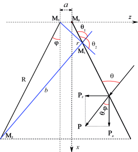
Figure 1: The schematic view of the configuration with nonparallel plates (wings) with the wing surface length $R$. The configuration section shown in the Cartesian coordinates in the plane $(x,z)$ has the width $L$ in the $y$ -direction normal to the plane of the figure. The blue straight lines indicate virtual rays with the length $b$ outgoing from the point $\mbox{M}_{1}$ at the limit angles $\Theta_{1}$ and $\Theta_{2}$ to the right wing and terminating at the ends of the opposite wing of the configuration at the points $\mbox{M}_{2}$ and $\mbox{M}_{3}$, respectively.

Let us consider a configuration with nonparallel plates, which will be used for the demonstration of the possibility in principle of the Casimir EMF existence. The outer and inner surfaces of the wings should have the properties of perfect mirrors. The configuration can be immersed into the material medium or be its part with the parameters of dielectric permittivity different from that of the physical vacuum. The configuration in the Cartesian coordinates looks like two thin metal plates with the width $L$ (oriented along the $z$ - axis) and surface length $R$; the plates are arranged at the distance $a$ from one another and the angle of the opening $2\varphi$ between them can be varied by the same value $\varphi$ simultaneously for the two wings of the configuration as shown in Fig.1. The particular case is parallel planes for $\varphi=0$ and a triangle at $a=0$.

Further, assuming that at any frequency $\omega$, the rays incident onto the plate from opposite sides at an arbitrary point $r$ are strictly oppositely directed, let us note the following. If we assume that the plates are very thin (one atomic layer), the local pressure produced by the opposite rays at the point $r$ inside the plate can be added vectorially. In this case the virtual ray producing the total pressure $P(r)$ Fateev:1 on the thin plate subsystem will act upon electrons. It is clear that the total $P(r)$ will correspond to the Casimir pressure at the given point $r$ of the incidence of the ray at the angle ${\Theta}^{\prime}$ to the normal of the wing surface. For finding EMF in the entire plate in the configuration it is necessary to find the sum of micro-EMF at all the point areas of the plate.

For the first approximation let us use the following known formula for the current strength due to the electron drag in metals Goff:1997 ; Goff:2000

$$\int{d\xi\left\langle{J_{\left\|\right.}}\right\rangle}=\sigma_{o}\frac{\left\langle S\right\rangle}{n_{b}ec}\left({1-\rho}\right)\sin{\Theta}^{\prime}\cos{\Theta}^{\prime}.$$ (1)

Here $\left\langle S\right\rangle$ is average density of the Poynting flux along the incidence of the monochromatic ray at the frequency $\omega$, $\sigma_{o}$ is specific conductivity of metal at constant current, $n_{b}$, $e$ are volume density and electron charge, $\rho$ is reflection coefficient, $c$ is light speed, and $\left\langle{J_{\left\|\right.}}\right\rangle$ is averaged current generated parallel to the plate surface per unit of its thickness $d\xi$. Further, for the ultrathin plate of the configuration, let us make a simplifying assumption that

$$\int{d\xi\left\langle{J_{\left\|\right.}(\xi)}\right\rangle}\approx\xi\left\langle{J_{\left\|\right.}}\right\rangle.$$

The Poynting flux density is expressed through the average density of the energy of the electromagnetic wave $\left\langle w\right\rangle$ Ditchburn:1953

$$\left\langle w\right\rangle=\frac{1}{c}\left\langle S\right\rangle,$$

In this case, the effective pressure on the surface at the mirror reflection from it is determined as follows

$$P=2\left\langle w\right\rangle=\frac{2}{c}\left\langle S\right\rangle.$$ (2)

The use of the simple relations of the type (2) prevents the necessity to calculate the Poynting fluxes for virtual electromagnetic waves at all possible frequencies $\omega$ because in all the formulae of the Casimir pressure all of them are taken into account anyhow. In addition, in the presented statement of the EMF problem we confine ourselves to the first approximation with no account taken of the possible difference in angles and degrees of wave reflection at different frequencies and other possible and required further corrections.

missing

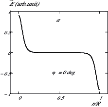
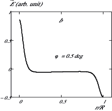
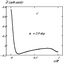
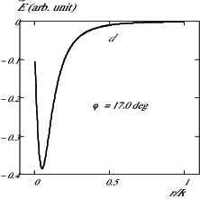
Figure 2: The electric field strengths $E(r)$ at local points $r$ on the configuration wing with the length $r_{\max}=R$ for four different angles $\varphi$.

Thus, taking into account the transmission coefficient of the plate $k$, expression (1) can be written in the form

$$\left\langle{J_{\left\|\right.}}\right\rangle=\sigma_{o}\frac{P(\Theta)}{2n_{b}e\xi}\left[{1-\rho-k}\right]\sin{\Theta}^{\prime}\cos{\Theta}^{\prime}.$$ (3)

Since electric current is associated with the electric field intensity $E$ through the simple relation

$$\vec{J}_{\parallel}=\sigma\vec{E}_{\parallel},$$

at the local point area we find

$$\vec{E}_{\parallel}=\frac{P(\Theta)}{2n_{b}e\xi}\left[{1-\rho-k}\right]\sin{\Theta}^{\prime}\cos{\Theta}^{\prime}.$$ (4)

Here the total Casimir pressure $P(\Theta)$ at the point $r$ is also dependent on the incidence angle $\Theta$ and can be borrowed from Ref. Fateev:1 . Let us note that the $\Theta$ angles for the presented geometry of the problem in Fig.1 are determined differently in contrast to the ${\Theta}^{\prime}$ angles for formulae (3) and (4) in Refs. Goff:1997 ; Goff:2000 . As seen from Fig.1, the overdetermination of the angles ${\Theta}^{\prime}$ and $\Theta$ obeys the rule

$${\Theta}^{\prime}=\left\{{{\begin{array}[]{*{20}c}{\textstyle{\pi\over 2}-\Theta;\;\Theta<\textstyle{\pi\over 2\hfill}}\\ {\Theta-\textstyle{\pi\over 2};\;\Theta>\textstyle{\pi\over 2\hfill}}\\ \end{array}}}\right.,$$ (5)

and consequently, the trigonometric term in formula (4) should be rewritten as follows

$$\sin{\Theta}^{\prime}\cos{\Theta}^{\prime}=\sin\Theta\cos\Theta.$$

Thus, EMF can be generated at the point $r$ on each area of the wings

$$\Delta E_{\parallel}=\int_{0}^{L}{dy}\int_{\Theta_{1}}^{\Theta_{2}}{\vec{E}_{\parallel}dr}.$$ (6)

The total EMF for the generation areas along the entire length of the wing with the length $r_{\max}$ is determined according to the rules of the series connection of the sources of EMF

$$\Delta E_{\parallel}=\frac{1}{2n_{b}e\xi}\left[{1-\rho-k}\right]\int_{0}^{L}{dy}\int_{0}^{r_{\max}}{P(\Theta,r,\varphi)dr}.$$ (7)

Here, the local specific pressure $P(\Theta,r,\varphi)$ at each point $r$ on the configuration wing with the length $r_{\max}$and width $L$ has the form similar to the expression found in Fateev:1 ; however, the term of the type $\cos(\Theta-\varphi)$ responsible for the $x\quad-$and $y\quad-$action of the Casimir forces on the tangential component (parallel to the wing plane) is replaced by the term of the form $\sin\Theta\cos\Theta$

$$\begin{array}[]{c}P(\Theta,r,\varphi)=-\frac{\hbar c\pi^{2}}{240s^{4}}\int_{\Theta_{1}}^{\Theta_{2}}{d\Theta}\sin(\Theta-2\varphi)^{4}\sin\Theta\cos\Theta\\ =-\frac{\hbar c\pi^{2}}{240s^{4}}A(\varphi,\Theta_{1},\Theta_{2}),\\ \end{array}$$ (8)

missing

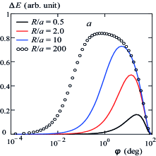
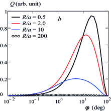
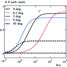
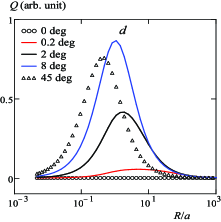
Figure 3: ($a$) and ($b$) – the EMF generated in the wing and the effectiveness $Q$ depending on the $\varphi$ angles for some lengths $R$. ($c)$ and ($d)$ – EMF and $Q$ effectiveness depending on the wing length $R$ for some $\varphi$ angles.

where

$$\begin{array}[]{c}A(\varphi,\Theta_{1},\Theta_{2})=\frac{1}{96}\left[{24\Theta_{1}\sin 4\varphi-24\Theta_{2}\sin 4\varphi}\right.\\ +18\cos 2\Theta_{1}-18\cos 2\Theta_{2}\\ +6\cos(4\varphi-4\Theta_{2})-6\cos(4\varphi-4\Theta_{1})\\ +3\cos(8\varphi-2\Theta_{2})-3\cos(8\varphi-2\Theta_{1})\\ \left.{+\cos(8\varphi-6\Theta_{1})-\cos(8\varphi-6\Theta_{2})}\right].\\ \end{array}$$ (9)

In formula (8), $\hbar=h/2\pi$ is the reduced Planck constant, $c$ is the light speed, and the functional expressions for the limit angles $\Theta_{1},\Theta_{2}$ in the configuration and the parameter $s$ have the forms

$$\begin{array}[]{c}\Theta_{1}=\mbox{arccos}\left[{-\frac{r+a\sin\varphi-R\cos 2\varphi}{\sqrt{\left({a+R\sin\varphi+r\sin\varphi}\right)^{2}+\left({r\cos\varphi-R\cos\varphi}\right)^{2}}}}\right],\end{array}$$ (10)

$$\Theta_{2}=\mbox{arccos}\left[{-\frac{r+a\sin\varphi}{\sqrt{a^{2}+r^{2}+2ra\sin\varphi}}}\right],$$ (11)

$$s=\frac{\sin(2\varphi-\Theta_{2})(a+r\sin\varphi)}{\sin(\varphi-\Theta_{2})}.$$ (12)

Thus, here a fundamental (idealized) model is presented for the calculation of the EMF generation in metal nanosized configurations due to virtual photons in optical approximation.

RESULTS

The use of formulae (5– 12) allows to reveal the following EMF character for two wings with the same length $R$ and minimal distance between them $a=4\times 10^{-9}$ m (see Fig.2). The same character of the dependences will be observed at the rescaling of the configuration dimensional parameters to any values, but naturally, for the ranges restricted by the distances between the atoms of well-conducting metals.

In Fig.2a it is seen that even when the configuration has parallel plates ($\varphi=0)$, on the ends of both the right and left wing, electric field is generated. The local field strength increases closer to the wing ends and on different ends it has opposite direction. In this case, EMF in any of the two parallel plates is not generated because of $\Delta E_{\parallel}=E_{{}_{\parallel}}^{+}+E_{{}_{\parallel}}^{-}=0$. However, at the slightest change of the $\varphi$ angle, noncompensation of the local magnitudes $E_{{}_{\parallel}}^{+}$ and $E_{{}_{\parallel}}^{-}$ appears (Fig.2b). At the further growth of the $\varphi$ angle, the noncompensation increases significantly (Fig.2c and 2d), which leads to the generation of EMF in the wings, which is the same in the direction and value. The current of dragged electrons in both wings is directed to the approaching ends of the configuration.

In accordance with formula (5), the integral quantity of EMF in each of the wings depends on the length $r_{\max}=R$ and $\varphi$ angles and has the form shown in Fig.3 a, b, c.

missing

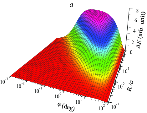
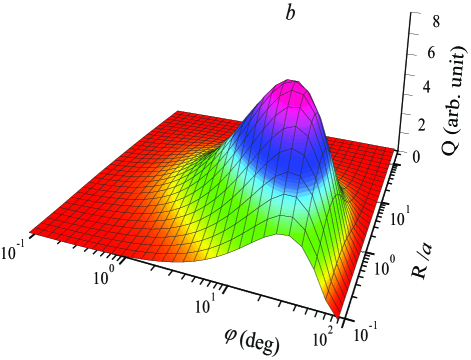
Figure 4: The generated EMF ($a$) in one separate wing of the configuration, and the configuration effectiveness (b) $Q$ depending on the $\varphi$ angles and wings lengths $R$.

From Fig.3 it follows that at the angle $\varphi=0$, EMF is not generated at any wing length $R$. However, at any of the angles $0<\varphi<\pi/2$, EMF is generated in any of the wings, and it grows with the increase of the length $R$. However, at some values of $R>R_{p}$, the EMF growth in the wing ceases. It means that the main contribution into the EMF generation is made by the end areas of the wings, mainly near the ends of the nonparallel wings forming the trapezoid configuration. It is clear that there is some optimal length of the wings $R$ and optimal angles $\varphi$ (Fig.3b,d), at which there is the maximum of the effectiveness function ratio

$$Q=\Delta E/R.$$ (13)

The effectiveness function maximum shifts with a decrease in the wing length $R$ to the large angles $\varphi$ and becomes smaller in its value at the same time. All the effects can be observed in two-dimensional dependences $\Delta E(R,\varphi)$ and $Q(R,\varphi)$ as it is shown in Fig.4.

Apparently, the excitation of EMF can also be expected in other open nanosized configurations. The demonstration of such possibility in two closely spaced metal plates is presented as the case which is the simplest and most available for calculation. Naturally, when the thickness, roughness, temperature and other real parameters of the plates are taken into account, the expected value of EMF in the configuration will significantly vary.

CONLUSION

Thus, in the present paper, the basic mechanism of the Casimir EMF generation in metal open nanosized configurations due to virtual photons has been presented. This possibility is theoretically demonstrated using flat metal plates (wings) angularly related to one another. In strictly parallel plates, EMF is not generated. However, EMF should be generated at any angles between the plates in the range of $0<\varphi<\pi/2$ reaching its maximum at certain average angles for any wing length. EMF is generated in both wings and has similarly situated poles. The optimal values for the wing lengths and angles between them have been found, at which the most effective EMF generation can take place.

- (1) H. B. G. Casimir, Kon. Ned. Akad. Wetensch. Proc. 51, 793 (1948).
- (2) H. B. G. Casimir and D. Polder, Phys. Rev. 73, 360 (1948).
- (3) K. A. Milton, The Casimir effect: Physical manifestations of zero-point energy, World Scientic, Singapore, 2001.
- (4) G. L. Klimchitskaya, U. Mohideen, V. M. Mostapanenko, Rev. Mod. Phys. 81, 1827 (2009).
- (5) M. Bordag, G. L. Klimchitskaya, U. Mohideen, and V.M. Mostepanenko, Advances in the Casimir effect, Oxford University Press, Oxford, 2009.
- (6) E. G. Fateev,arXiv:1208.0303 [quant-ph].
- (7) E. G. Fateev,arXiv:1301.1110 [quant-ph].
- (8) E. G. Fateev,arXiv:1208.1256 [quant-ph].
- (9) G. Bimonte, J. Phys. A 41, 164013 (2008).
- (10) V. L. Gurevich, R. Laiho, A. V. Lashkul, Phys. Rev. Lett. 69, 180 (1992).
- (11) V.M. Shalaev, C. Douketis, M. Moskovits, Phys. Lett. A 169, 205 (1992).
- (12) V. M. Shalaev, C. Douketis, J. T. Stuckless, M. Moskovits, Phys. Rev. B 53, (1996).
- (13) G. M. Mikheev, A. G. Nasibulin, R.G. Zonov, A. Kaskela, and E. I. Kauppinen, Nano Lett. 12, 77 (2012).
- (14) V. L. Al’perovich, V. I. Belinicher, V. N. Novikov, A. S. Terekhov, Pis’ma Zh. Eksp. Teor. Fiz. 33, 573 (1981) JETP Lett, 33(11), 5 (1981).
- (15) J. E. Goff , W. L. Schaich, Phys. Rev. B 56 (23), 15421 (1997).
- (16) J. E. Goff, W. L. Schaich, Phys. Rev. B 61, 10471 (2000).
- (17) R. W. Ditchburn. Light. Interscience, New York, 1953.