Cutting Stock with Binary Patterns:
Arc-flow Formulation with Graph Compression

Abstract

The cutting stock problem with binary patterns (0-1 CSP) is a variant of CSP that usually appears as a relaxation of 2D and 3D packing problems. We present an exact method, based on an arc-flow formulation with side constraints, for solving 0-1 CSP by simply representing all the patterns in a very compact graph.

Gilmore-Gomory’s column generation approach is usually used to compute strong lower bounds for 0-1 CSP. We report a computational comparison between the arc-flow approach and the Gilmore-Gomory’s approach.  
Keywords: Bin Packing, Cutting Stock, Strip Packing, Arc-flow Formulation

1 Introduction

The cutting stock problem (CSP) is a combinatorial NP-hard problem (see, e.g., Garey and Johnson, 1979) in which pieces of different widths must be cut from rolls in such a way that the waste is minimized. In this problem, we are given the width $W$ of the rolls, a set of $m$ piece widths $w$ and their demands $b$. Since all the rolls have the same width and demands must be met, the objective is equivalent to minimizing the number of rolls that are used. In the cutting stock problem with binary patterns (0-1 CSP) items of each type may be cut at most once in each roll. In the 0-1 CSP, pieces are identified by their types and some types may have the same width.

The 2D strip packing problem (SPP) is another combinatorial NP-hard problem. In this problem, we are given a half-open strip of width $W$ and we want to minimize the height needed to pack a set of 2D rectangular items. An known lower bound for SPP is the bar relaxation of Scheithauer, (1999), which corresponds to the minimum number of one-dimensional packing patterns in width direction (bar patterns with length one) that are required to hold all the items. This relaxation corresponds to a cutting stock problem with binary patterns (0-1 CSP) since each bar contains at most one slice of each item. For 3D problems, there are bar and slice relaxations (see, e.g., Belov et al., 2009), both of which are also 0-1 CSP problems.

The 0-1 CSP can be reduced and solved as a vector packing problem with $m+1$ dimensions, one for the capacity constraint and $m$ binary dimensions to ensure that each pattern contains at most one item of each type. Brandão, (2012) presents a graph compression method for vector packing arc-flow graphs that usually leads to large reductions in the graph size. In this paper, we use a different method for introducing binary constraints in arc-flow models that only requires a single additional dimension. The main contributions of this paper are: we present a exact method for solving 0-1 CSP with binary patterns which can be easily generalized for vector packing with binary patterns. This generalization allows, for instance, modeling 0-1 CSP with conflicts, which is another problem that usually appears when solving 2D and 3D packing problems.

The remainder of this paper is organized as follows. Section 2 presents underlying mathematical optimization models, and Section 3 the arc-flow approach to 0-1 CSP. Some computational results are presented in Section 4 and Section 5 presents the conclusions.

2 Mathematical optimization models

Gilmore and Gomory, (1961) proposed the following model for the standard CSP. A combination of orders in the width of the roll is called a cutting pattern. Let column vectors $a^{j}=(a_{1}^{j},\ldots,a_{m}^{j})^{\top}$ represent all possible cutting patterns $j$. The element $a_{i}^{j}$ represents the number of rolls of width $w_{i}$ obtained in cutting pattern $j$. Note that in the standard CSP, the patterns are non-negative integer vectors; in the 0-1 CSP, only binary patterns are allowed. Let $x_{j}$ be a decision variable that designates the number of rolls to be cut according to cutting pattern $j$. The 0-1 CSP can be modeled in terms of these variables as follows:

minimize $$\sum_{j\in J}x_{j}$$ (1)

subject to $$\sum_{j\in J}a_{i}^{j}x_{j}\geq b_{i},\qquad i=1,\ldots,m,$$ (2)

$$x_{j}\geq 0,\mbox{ integer},\qquad \forall j\in J,$$ (3)

where $J$ is the set of valid cutting patterns that satisfy:

$$\sum_{i=1}^{m}a_{i}^{j}w_{i}\leq W\mbox{ and }a_{i}^{j}\in\{0,1\}.$$ (4)

It may be impractical to enumerate all the columns in the previous formulation, as their number may be very large, even for moderately sized problems. To tackle this problem, Gilmore and Gomory, (1963) proposed column generation.

Let the linear optimization of Model (1)-(3) be the restricted master problem. At each iteration of the column generation process, a subproblem is solved and a column (pattern) is introduced in the restricted master problem if its reduced cost is strictly less than zero. The subproblem, which is a knapsack problem, is the following:

minimize $$1-\sum_{i=1}^{m}c_{i}a_{i}$$ (5)

subject to $$\sum_{i=1}^{m}w_{i}a_{i}\leq W$$ (6)

$$a_{i}\in\{0,1\},\ i=1,\ldots,m,$$ (7)

where: $c_{i}$ is the shadow price of the demand constraint of item $i$ obtained from the solution of the linear relaxation of the restricted master problem, and $a=(a_{1},\ldots,a_{m})$ is a cutting pattern whose reduced cost is given by the objective function.

The column generation process for this method can be summarized as follows. We start with a small set of patterns (columns), which can be composed by $m$ patterns, each containing a single, different item. Then we solve the linear relaxation of the restricted master problem with the current set of columns. At each iteration, a knapsack subproblem is solved and the pattern $a^{*}$ from its solution is introduced in the restricted master problem. Simplex iterations are then performed to update the solution of the master problem. This process is repeated until no pattern with negative reduced cost is found. At the end of this process, we have the optimal solution of the linear relaxation of the model (1)-(3).

Model (5)-(7) corresponds to a 0-1 knapsack problem that can be solved in pseudo-polynomial time with dynamic programming using Algorithm 1, that runs in $\mathcal{O}(Wm)$ time.

Consider a 0-1 CSP instance with bins of capacity $W=8$ and items of sizes 4, 3, 2. The dynamic programming search space of Algorithm 1 is represented in Figure 1, and it corresponds to a directed acyclic graph in which every valid packing pattern is represented as a path from s to t. Brandão, (2012) presents a general arc-flow formulation, equivalent to Model (1)-(4), that can be used to solve 0-1 CSP directly as a minimum flow problem between s and t, with additional constraints enforcing the sum of the flows in the arcs of each item to be greater than or equal to the corresponding demand. This general arc-flow formulation is a generalization of the model proposed in Valério de Carvalho, (1999) and it only requires a directed acyclic graph containing every valid packing pattern represented as a path between two vertices to solve the corresponding cutting stock problem. The lower bound provided by this formulation is the same as the one provided by Gilmore-Gomory’s model with the same set of patterns (see, e.g., Brandão, 2012). A simplified version of the general arc-flow formulation is the following:

minimize $$z$$ (8)

subject to $$\sum_{(u,v,i)\in A}f_{uvi}-\sum_{(v,u^{\prime},i)\in A}f_{vu^{\prime}i}= \left\{\begin{array}[]{rl}-z&\mbox{if }v=\textsc{s},\\ z&\mbox{if }v=\textsc{t},\\ 0&\mbox{for }v\in V\setminus\{\textsc{s},\textsc{t}\},\\ \end{array}\right.$$ (12)

$$\sum_{(u,v,i)\in A}f_{uvi}\geq b_{i}, i\in\{1,\ldots,m\},$$ (13)

$$f_{uvi}\geq 0,\mbox{ integer}, \forall(u,v,i)\in A,$$ (14)

where: $m$ is the number of different items; $b_{i}$ is the demand of the $i$-th item; $V$ is the set of vertices, s is the source vertex and t is the target; $A$ is the set of arcs, each arc having components $(u,v,i)$ corresponding to an arc between nodes $u$ and $v$ that contributes to the demand of the $i$-th item; arcs $(u,v,i=0)$ are loss arcs that represent unoccupied portions of the patterns; $f_{uvi}$ is the amount of flow along the arc $(u,v,i)$; and $z$ is a variable that can be seen as a feedback arc from vertex t to s. Note that this formulation allows multiple arcs between the same pair of vertices.

1

2

3

input : $m$ - number of different items; $w$ - item sizes; $v$ - item values; $W$ - capacity limit

output : maximum profit

4

5function $\textnormal{{knapsack}}(m,w,v,W)$:

6       for $p=0$ to $W$ do $\textnormal{{dp}}[0,p]\leftarrow 0$;  // base cases

7       for $i=1$ to $m$ do // for each item

8             for $p=0$ to $W$ do // for each position

9                   if $p<w_{i}$ then $\textnormal{{dp}}[i,p]\leftarrow\textnormal{{dp}}[i-1,p]$; 

10                   else $\textnormal{{dp}}[i,p]\leftarrow\max(\textnormal{{dp}}[i-1,p],\textnormal{{dp}}[i-1,p-w_{i}]+v_{i})$; 

11                  

12            

13       return $\max_{p=0..W}\{\textnormal{{dp}}[m,p]\}$;

14      

Algorithm 1 0-1 Knapsack Algorithm

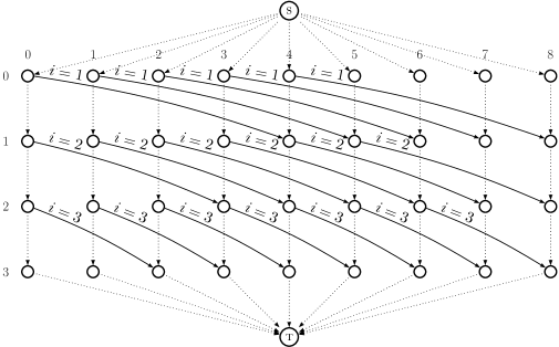
Figure 1: Dynamic programming graph for a knapsack instance with capacity 8 and items of sizes 4, 3, 2.

3 Arc-flow formulation with graph compression for 0-1 CSP

Consider a 0-1 CSP instance with bins of capacity $W=8$ and items of sizes 4, 3, 2 with demands 3, 2, 5, respectively. Since a pattern is a set of items, in order to avoid redundant patterns we will assume that this set is ordered, and consider only patterns in which the items are ordered by decreasing values of the index in this set. Figure 2 shows a graph which contains every valid packing pattern (respecting that order) for this instance represented as path from the source s to the target t. In this graph, a node label $(a^{\prime},b^{\prime})$ means that every sub-pattern from the source to the node uses no more than $a^{\prime}$ space and contains no item with an index higher than $b^{\prime}$. This graph can be seen as the Step-1 graph of Brandão, (2012)’s method. The dashed arcs are the loss arcs that represent unoccupied portions of the patterns, which can be seen as items with no width ($w_{0}=0$). In a general arc-flow graph, a tuple $(u,v,i)$ corresponds to an arc between nodes $u$ and $v$ associated with the $i$-th item. Note that, for each pair of nodes $(u,v)$, multiple arcs, each associated with a different item, are allowed.

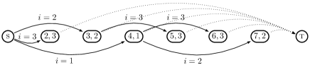
Figure 2: Initial graph/Step-1 graph.

Graph corresponding to a 0-1 CSP instance with bins of capacity $W=8$ and items of sizes 4, 3, 2 with demands 3, 2, 5, respectively.

Brandão, (2012) presents a three-step graph compression method whose first step consists of breaking the symmetry by dividing the graph into levels. The way used to represent patterns in Figure 2 does not allow symmetry. The graph division by levels does not improve this, but it increases the flexibility of the graph and usually allows substantial improvements in the compression ratio. Note that this graph division by levels does not exclude any valid packing pattern that respects the order (see, e.g., Brandão, 2012). It is easy to check that, excepting loss, for every valid packing pattern in the initial graph, there is a corresponding path in the Step-2 graph.

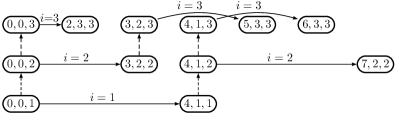
Figure 3: Graph with levels/Step-2 graph.

The Step-2 graph has 13 nodes and 22 arcs (considering also the final loss arcs connecting internal nodes to t, which were omitted). In this graph, $\textsc{s}=(0,0,1)$.

In the main compression step, a new graph is constructed using the longest path to the target in each dimension. In our case, we use in the first dimension the longest path from the node to the target, and in the second the highest item index that appears in any path from the node to the target. Let ($\varphi(u)$, $\psi(u)$) be the label of node $u$ in the first and second dimensions, respectively. We define $\varphi(u)$ and $\psi(u)$ as follows:

$$\varphi(u) = \left\{\begin{array}[]{ll}W&\mbox{if }u=\textsc{t},\\ \min_{(u^{\prime},v,i)\in A:u^{\prime}=u}\{\varphi(v)-w_{i}\}&\mbox{otherwise.}\\ \end{array}\right.$$ (17)

$$\psi(u) = \left\{\begin{array}[]{ll}\infty&\mbox{if }u=\textsc{t},\\ \min(\min_{(u^{\prime},v,i)\in A:u^{\prime}=u}\{\psi(v)\},\min_{(u,v,i\neq 0)\in A}\{i\})&\mbox{otherwise.}\\ \end{array}\right.$$ (20)

In the paths from s to t in Step-2 graph usually there is some float. In this process, we are moving this float as much as possible to the beginning of the paths. The label in each dimension of every node $u$ corresponds to the highest value in each dimension where the sub-patterns from $u$ to t can start so that the constraints are not violated. Figure 4 shows the graph that results from applying the main compression step to the graph of Figure 3.

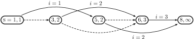
Figure 4: Step-3 graph (after the main compression step).

The Step-3 graph has 8 nodes and 17 arcs (considering also the final loss arcs connecting internal nodes to t, which were omitted).

In the final compression step, a new graph is constructed once more, using in the first dimension the longest path from the source to the current node, and in the second the highest item index that appears in any path from the source to the current node. Figure 5 shows the final graph. Let ($\varphi^{\prime}(v)$, $\psi^{\prime}(v)$) be the label of node $v$ in the first and second dimensions, respectively. We define $\varphi^{\prime}(v)$ and $\psi^{\prime}(v)$ as follows:

$$\varphi^{\prime}(v) = \left\{\begin{array}[]{ll}0&\mbox{if }v=\textsc{s},\\ \max_{(u,v^{\prime},i)\in A:v^{\prime}=v}\{\varphi^{\prime}(u)+w_{i}\}&\mbox{otherwise.}\\ \end{array}\right.$$ (23)

$$\psi^{\prime}(v) = \left\{\begin{array}[]{ll}0&\mbox{if }v=\textsc{s},\\ \max_{(u,v^{\prime},i)\in A:v^{\prime}=v}\{\max(\psi^{\prime}(u),i)\}&\mbox{otherwise.}\\ \end{array}\right.$$ (26)

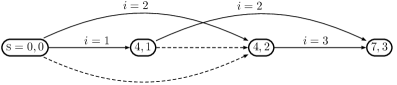
Figure 5: Step-4 graph (after the final compression step).

The Step-4 graph has 5 nodes and 9 arcs (considering also the final loss arcs connecting internal nodes to t, which were omitted). The initial Step-1 graph had 8 nodes and 12 arcs.

The problem of minimizing the flow $z$ in the final graph is solved by a general-purpose mixed-integer optimization solver. The graph compression usually leads to very small graphs. However, Step-2 graph can be large and the three-step graph compression method may take too long. Note that 0-1 CSP problems may need to be solved many times, for instance, as bar or slices relaxations during the solution of 2D and 3D packing problems, and hence it is very important to build the models as quick as possible. Algorithm 2 builds the Step-3 graph directly using a recursive procedure with memoization. The base idea for this algorithm comes from the fact that in the main compression step the label of any node only depends on the labels of the two nodes to which it is connected (a node in its level and another in level above). After directly building the Step-3 graph from the instance’s data using this algorithm, we just need to apply the final compression step to obtain the final graph. This method allows us to obtain arc-flow models even for large benchmark instances in a few milliseconds.

1

2

3

input : $m$ - number of different items; $w$ - item sizes; $W$ - capacity limit

output : $V$ - set of vertices; $A$ - set of arcs; s - source; s - target

4

5function $\textnormal{{buildGraph}}(m,w,W)$:

6       $V\leftarrow\{\ \}$; $A\leftarrow\{\ \}$;

7       $\textnormal{{dp}}[x^{\prime},i^{\prime}]\leftarrow\textnormal{{NIL}},\mbox{ \bf for all }x^{\prime},i^{\prime}$;

8       function $\textnormal{{build}}(x,i)$:

9             if $\textnormal{{dp}}[x,i]\neq\textnormal{{NIL}}$ then // avoid repeating work

10                   return $\textnormal{{dp}}[x,i]$;

11                  

12             $(u_{x},u_{i})\leftarrow(W,m+1)$;

13             if $i<m$ then // option 1: do not use the current item

14                   $(up_{x},up_{i})\leftarrow\textnormal{{build}}(x,i+1)$;

15                   $(u_{x},u_{i})\leftarrow(up_{x},up_{i})$;

16                  

17             if $x+w_{i}\leq W$ then // option 2: use the current item

18                   $(v_{x},v_{i})\leftarrow\textnormal{{build}}(x+w_{i},i+1)$;

19                   $(u_{x},u_{i})\leftarrow(\min(u_{x},v_{x}-w_{i}),i)$;

20                   $A\leftarrow A\cup\{((u_{x},u_{i}),(v_{x},v_{i}),i)\}$;

21                   $V\leftarrow V\cup\{(u_{x},u_{i}),(v_{x},v_{i})\}$;

22                   if $i<m$ and $u\neq up$ then

23                         $A\leftarrow A\cup\{((u_{x},u_{i}),(up_{x},up_{i}),0)\}$;

24                         $V\leftarrow V\cup\{(up_{x},up_{i})\}$;

25                        

26                  

27             $\textnormal{{dp}}[x,i]\leftarrow(u_{x},u_{i})$;

28            

29            return $(u_{x},u_{i})$;

30            

      $\textsc{s}\leftarrow\textnormal{{build}}(0,1)$;

        // build the graph

31       $V\leftarrow V\cup\{\textsc{t}\}$;

       $A\leftarrow A\cup\{(u,\textsc{t},0)\ |\ u\in V\setminus\{\textsc{s},\textsc{t}\}\}$;

        // connect internal nodes to the target

32       return $(G=(V,A),\textsc{s},\textsc{t})$;

33      

Algorithm 2 Direct Step-3 Graph Construction Algorithm

4 Computational results

We used the arc-flow formulation to compute the bar relation of the two-dimensional bin packing test data of Lodi et al., (1999). This data set is composed by ten classes; the first six were proposed by Berkey and Wang, (1987), and the last four were proposed by Martello and Vigo, (1998). In the bar relaxations, the item widths are the original widths and the demand is given by the original height of the item. The characteristics of the first six classes are summarized as follows: Class I: $W=10$, $w_{i}\in[1,10]$ and $b_{i}\in[1,10]$; Class II: $W=30$, $w_{i}\in[1,10]$ and $b_{i}\in[1,10]$; Class III: $W=40$, $w_{i}\in[1,35]$ and $b_{i}\in[1,35]$; Class IV: $W=100$, $w_{i}\in[1,35]$ and $b_{i}\in[1,35]$; Class V: $W=100$, $w_{i}\in[1,100]$ and $b_{i}\in[1,100]$; Class VI: $W=300$, $w_{i}\in[1,100]$ and $b_{i}\in[1,100]$. In each of the previous classes, all the item sizes are generated in the same interval. In the next four classes, item sizes are generated from different intervals. The characteristics of 70% of the items in each class are summarized as follows: Class VII: $W=100$, $w_{i}\in[66,100]$ and $b_{i}\in[1,50]$; Class VIII: $W=100$, $w_{i}\in[1,50]$ $b_{i}\in[66,100]$; Class IX: $W=100$, $w_{i}\in[50,100]$ $b_{i}\in[50,100]$; Class X: $W=100$, $w_{i}\in[1,50]$ $b_{i}\in[1,50]$.

Table 1 presents a comparison between Gilmore-Gomory’s column generation approach and the arc-flow formulation approach. The meaning of each column is as follows: $W$ - strip width; $m$ - number of different items; CSP - optimal standard CSP solution; $z_{\mathop{\mathrm{lp}}}$ - LP lower bound; $z_{\mathop{\mathrm{ip}}}$ - optimal 0-1 CSP solution; $\mathop{\#\mathrm{cols}}$ - number of columns used in the column generation approach; $\#v$, $\#a$ - number of vertices and arcs in the arc-flow graph; $\%v$, $\%a$ - ratios between the numbers of vertices and arcs of the arc-flow graph and the ones of the straightforward dynamic programming graph presented in Section 2; $t^{\mathop{\mathrm{gg}}}$ - column generation run time; $t^{\mathop{\mathrm{af}}}_{\mathop{\mathrm{lp}}}$, $t^{\mathop{\mathrm{af}}}_{\mathop{\mathrm{ip}}}$ - run time of the arc-flow approach (linear relaxation and integer solution); $\#{\mathop{\mathrm{gg}}}$, $\#{\mathop{\mathrm{af}}}$ - number of instances that were solved in $\min(t^{\mathop{\mathrm{gg}}},t^{\mathop{\mathrm{af}}}_{\mathop{\mathrm{lp}}})$ seconds using each method. The values shown are averages over the 10 instances in each class. CPU times were obtained using a computer with two Quad-Core Intel Xeon at 2.66GHz, running Mac OS X 10.8.0. All the algorithms were implemented in C++, and Gurobi 5.0.0 (Gu et al., 2012), a state-of-the-art mixed integer programming solver, was used as LP and ILP solver. The source code is available online.

[b] Class $W$ $m$ CSP $z_{\mathop{\mathrm{ip}}}$ $z_{\mathop{\mathrm{lp}}}$ $\mathop{\#\mathrm{cols}}$ $\#v$ $\#a$ $\%v$ $\%a$ $t^{\mathop{\mathrm{gg}}}$ $t^{\mathop{\mathrm{af}}}_{\mathop{\mathrm{lp}}}$ $t^{\mathop{\mathrm{af}}}_{\mathop{\mathrm{ip}}}$ $\#{\mathop{\mathrm{gg}}}$ $\#{\mathop{\mathrm{af}}}$ I 10 20 60.4 60.8 60.6 47.8 23.6 87.3 0.1 0.24 0.01 0.01 0.01 0 10 I 10 40 121.2 121.7 121.4 105.3 56.1 214 0.12 0.31 0.02 0.01 0.01 0 10 I 10 60 188.5 188.5 188.3 147.3 80.8 318.8 0.12 0.31 0.03 0.01 0.02 0 10 I 10 80 262.6 262.6 262.2 189.8 105.3 417.9 0.12 0.31 0.04 0.01 0.02 0 10 I 10 100 304.8 304.8 304.3 297 163.3 629.2 0.15 0.38 0.1 0.01 0.03 0 10 II 30 20 19.7 19.7 19.3 45.5 131.9 436.3 0.2 0.36 0.01 0.01 0.06 9 4 II 30 40 39.1 39.1 38.7 93.1 357.9 1190.4 0.28 0.51 0.02 0.03 0.46 9 1 II 30 60 60.1 60.1 59.8 139 602.8 2008.9 0.32 0.58 0.04 0.05 2.01 8 2 II 30 80 83.2 83.2 82.7 188 812.9 2719.7 0.32 0.6 0.07 0.07 3.2 3 7 II 30 100 100.5 100.5 99.9 240.6 1131.1 3727.4 0.36 0.65 0.13 0.11 3.03 0 10 III 40 20 160.1 161 160.8 50.4 44.3 166.7 0.05 0.12 0.01 0.01 0.01 1 10 III 40 40 330.4 331.6 331.3 108.4 141.5 539.8 0.08 0.2 0.02 0.01 0.02 0 10 III 40 60 502.6 503.4 503 169.3 224.5 888.9 0.09 0.23 0.04 0.02 0.05 0 10 III 40 80 707.2 707.2 706.9 228.1 308.8 1215.4 0.09 0.24 0.06 0.03 0.06 0 10 III 40 100 834.8 834.9 834.4 307.1 525.4 1973.5 0.13 0.3 0.12 0.05 0.19 0 10 IV 100 20 61.4 61.4 60.9 57 249.4 859.8 0.12 0.22 0.01 0.02 0.09 10 0 IV 100 40 123.9 123.9 123.3 107.1 866.7 2962.7 0.21 0.39 0.03 0.07 0.77 10 0 IV 100 60 193 193 192.4 158.5 1618.3 5502.5 0.26 0.49 0.06 0.16 2.11 10 0 IV 100 80 267.2 267.2 266.7 219.5 2209.2 7528.3 0.27 0.51 0.11 0.29 3.64 10 0 IV 100 100 322 322 321.4 280.2 3157 10545.7 0.31 0.57 0.2 0.46 11.51 10 0 V 100 20 515.5 530.2 530 42.5 39.8 150.4 0.02 0.05 0.01 0.01 0.01 2 10 V 100 40 1061.2 1069.1 1069.1 89.5 164.8 648.8 0.04 0.1 0.02 0.01 0.02 2 9 V 100 60 1625.1 1635.4 1635.2 153 307.8 1246.2 0.05 0.13 0.04 0.03 0.04 1 9 V 100 80 2281.4 2283.8 2283.4 197.9 461.6 1839.7 0.06 0.15 0.05 0.03 0.06 0 10 V 100 100 2634.3 2634.8 2634.4 296.1 875.8 3320.6 0.09 0.22 0.11 0.07 0.17 0 10 VI 300 20 159.9 159.9 159.4 69.2 412.6 1464.4 0.07 0.13 0.02 0.03 0.19 10 0 VI 300 40 323.5 323.5 323.1 126 2046.3 7010.3 0.17 0.31 0.04 0.24 2.2 10 0 VI 300 60 505.1 505.1 504.7 186.6 4220.4 14361.9 0.23 0.43 0.09 0.64 14.68 10 0 VI 300 80 699.7 699.7 699.1 255.4 5908.6 20153.3 0.24 0.45 0.17 1.1 20.45 10 0 VI 300 100 843.8 843.8 843.1 329.1 8646.9 28900.2 0.28 0.52 0.33 2.34 75.14 10 0 VII 100 20 484.9 500.6 500.6 25.9 9.2 37.5 0 0.01 0.01 0.01 0.01 5 10 VII 100 40 1050.7 1054.7 1054.6 55.2 21.2 98.6 0.01 0.02 0.01 0.01 0.01 3 10 VII 100 60 1513.3 1525 1524.9 87.9 48 219.9 0.01 0.03 0.01 0.01 0.01 2 10 VII 100 80 2210.6 2220.8 2220.7 117.4 78.1 374.4 0.01 0.03 0.01 0.01 0.01 0 10 VII 100 100 2633.3 2642.7 2642.6 151.1 152.8 656.5 0.01 0.05 0.02 0.01 0.02 0 10 VIII 100 20 437.4 437.9 437.3 60.6 97.7 364.9 0.05 0.1 0.01 0.01 0.02 2 9 VIII 100 40 922.7 924.7 924.1 121.2 351.4 1325.4 0.08 0.19 0.03 0.03 0.12 6 5 VIII 100 60 1360.9 1360.9 1360.5 191.8 776.4 2832.3 0.13 0.28 0.06 0.08 0.56 9 2 VIII 100 80 1911.4 1911.4 1911.1 257.5 1081.3 3977.6 0.13 0.3 0.11 0.14 0.9 8 2 VIII 100 100 2363 2363 2362.5 330.5 1708.7 6085.3 0.17 0.36 0.18 0.26 2.65 10 0 IX 100 20 1103.6 1106.8 1106.8 27.5 10.3 42.4 0 0.01 0.01 0.01 0.01 5 10 IX 100 40 2180.9 2190 2189.9 53.3 22.9 110.6 0.01 0.02 0.01 0.01 0.01 2 10 IX 100 60 3394 3410.4 3410.4 79.8 40.4 202.1 0.01 0.02 0.01 0.01 0.01 3 9 IX 100 80 4563.9 4584.4 4584.4 106.5 82.3 402.2 0.01 0.04 0.01 0.01 0.01 2 9 IX 100 100 5415.6 5431.2 5431.2 146.6 190.9 851.4 0.02 0.06 0.02 0.01 0.02 1 10 X 100 20 341.4 347.1 346.9 51.9 86.3 323.1 0.04 0.09 0.01 0.01 0.01 1 10 X 100 40 653.7 654.6 654.2 121.4 315.5 1191.8 0.08 0.18 0.03 0.03 0.07 2 8 X 100 60 918.4 919.5 919.2 213.3 752.9 2741.7 0.12 0.27 0.06 0.08 0.23 7 3 X 100 80 1185.3 1186 1185.3 311.5 1084.7 3970.9 0.13 0.3 0.13 0.16 0.39 5 5 X 100 100 1480.7 1480.7 1480.4 394.9 1650.1 5931.2 0.16 0.35 0.22 0.32 2.14 8 2 Summary 1030.4 1033.7 1033.3 156.6 889.1 3095.4 0.12 0.25 0.06 0.14 2.95 216 316

Table 1: Arc-flow results.

The arc-flow formulation is faster than Gilmore-Gomory’s approach in 284 instances, both methods present the same run time in 32 instances and Gilmore-Gomory’s approach is faster than the arc-flow approach in 184 instances. The hardest instances for the arc-flow approach are the ones of classes IV and VI since they mostly contain small items that lead to very long patterns. Graphs associated to this type of instances tend to be larger and the run times tend to be higher due to the larger number of variables and constraints.

In Gilmore-Gomory’s approach, we used dynamic programming to solve the knapsack problems. The arc-flow graph can also be used to solve knapsack problems. However, since $W$ and $m$ are small in this data set, a straightforward dynamic programming solution is faster due its very low constant factors and its good caching behavior. For instances with larger values of $W$ and $m$, the use of the arc-flow graph to solve the knapsack problems may improve substantially the run time.

The graph compression achieved very good reductions in these instances. The average ratios between the numbers of vertices and arcs of the arc-flow graph and the ones of the straightforward dynamic programming graph are $25\%$ and $6\%$, respectively. Moreover, there are instances whose corresponding compressed graph is more than one hundred times smaller than the dynamic programming graph. There are ten instances whose corresponding graph became so small that it was faster to solve them exactly than to compute the linear relaxation using Gilmore-Gomory’s approach. All the instances from this data set were solved exactly using the arc-flow method in less than 3 seconds, on average.

The standard CSP can be used as a relaxation of 0-1 CSP. However, the bound provided by 0-1 CSP is much stronger than the one provided by standard CSP. In this data set, the maximum difference between the two bounds is 49, a clear indication of the superiority of 0-1 CSP is better for assessing bar and slice relaxations.

There have been many studies (see, e.g., Scheithauer and Terno, 1995, Scheithauer and Terno, 1997) about the integrality gap of Gilmore-Gomory’s model for the standard cutting stock problem. The largest gap known so far is $7/6$ and it was found by Rietz et al., (2002). Scheithauer and Terno, (1997) conjecture that $z_{\mathop{\mathrm{ip}}}\leq\lceil z_{\mathop{\mathrm{lp}}}\rceil+1$ for the standard CSP. For the 0-1 CSP, Gilmore-Gomory model’s bounds are also very strong. Note that our arc-flow model is equivalent to Gilmore-Gomory’s model and hence the lower bounds provided by the linear relaxations are the same. The largest gap between the linear relaxation of the 0-1 CSP formulations and the exact solution is 0.99 in this data set. Therefore, the linear relaxation is usually enough when 0-1 CSP is used as a relaxation of other problems. Nevertheless, for other applications and other problems with binary constraints, the exact solution may be very important.

Kantorovich, (1960) introduced an assignment-based mathematical programming formulation for CSP, which can be easily modified for 0-1 CSP by restricting the variables to binary values. Assignment-based formulations are usually highly symmetric and provide very weak lower bounds (see, e.g., Brandão, 2012). Therefore, this type of models are usually very inefficient in practice. Using this assignment-based model, we were only able to solve 126 out of the 500 instances within a 10 minute time limit. Using the arc-flow formulation, all the instances were easily solved, spending 3 seconds per instance on average, and none of the instances took longer than 200 seconds to be solved exactly.

5 Conclusions

We propose an arc-flow formulation with graph compression for solving cutting stock problems with binary patterns (0-1 CSP), which usually appears as a relaxation of 2D and 3D packing problems. Column generation is usually used to obtain a strong lower bound for 0-1 CSP. To the best of our knowledge, we present for the first time an effective exact method for this problem. We also report a computational comparison between the arc-flow approach and the Gilmore-Gomory’s column generation approach for computing lower bounds.

Our method can be easily generalized for vector packing with binary patterns by using multiple capacity dimensions instead of just one. This generalization allows, for instance, modeling 0-1 CSP with conflicts, which is another problem that usually appears when solving 2D and 3D packing problems.

References

- Belov et al., (2009) Belov, G., Kartak, V., Rohling, H., and Scheithauer, G. (2009). One-dimensional relaxations and LP bounds for orthogonal packing. International Transactions in Operational Research, 16(6):745–766.
- Berkey and Wang, (1987) Berkey, J. and Wang, P. (1987). Two-dimensional finite bin-packing algorithms. J. Oper. Res. Soc., 38:423–429.
- Brandão, (2012) Brandão, F. (2012). Bin Packing and Related Problems: Pattern-Based Approaches. Master’s thesis, Faculdade de Ciências da Universidade do Porto, Portugal.
- Garey and Johnson, (1979) Garey, M. R. and Johnson, D. S. (1979). Computers and Intractability: A Guide to the Theory of NP-Completeness. W. H. Freeman & Co., New York, NY, USA.
- Gilmore and Gomory, (1963) Gilmore, P. and Gomory, R. (1963). A linear programming approach to the cutting stock problem–part II. Operations Research, 11:863–888.