Metallic Quantum Ferromagnets

Abstract

This review gives an overview of the quantum phase transition (QPT) problem in metallic ferromagnets, discussing both experimental and theoretical aspects. These QPTs can be classified with respect to the presence and strength of quenched disorder: Clean systems generically show a discontinuous, or first-order, QPT from the ferromagnetic state to a paramagnetic one as a function of some control parameter, as predicted by theory. Disordered systems are much more complicated, depending on the disorder strength and the distance from the QPT. In many disordered materials the QPT is continuous, or second order, and Griffiths-phase effects coexist with QPT singularities near the transition. In other systems the transition from the ferromagnetic state at low temperatures is to a different type of long-range order, such as an antiferromagnetic or a spin-density-wave state. In still other materials a transition to a state with glass-like spin dynamics is suspected. The review provides a comprehensive discussion of the current understanding of these various transitions, and of the relation between experimental and theoretical developments.

I Introduction

Metallic ferromagnets have been studied since ancient times, as this class of materials includes elemental iron, which gave ferromagnetism its name, as well as nickel and cobalt. Detailed studies in the early 1900s led to one of the first examples of mean-field theory Weiss (1907). A more elaborate version of mean-field theory by Stoner (1938) explained how a nonzero magnetization can arise from a spontaneous splitting of the conduction band. When it became clear, 30 years later, that mean-field theory does not correctly describe the behavior close to the phase transition, ferromagnetism became one of the testing grounds for the theory of critical phenomena Stanley (1971); Wilson and Kogut (1974). More recently metallic ferromagnets with low Curie temperatures, ranging from tens of degrees to a few degrees, or even lower, have attracted much attention. One motivation for the study of these materials is that many of them allow for decreasing the Curie temperature even further, by applying pressure or by changing the chemical composition. This allows the study of the quantum phase transition that occurs at zero temperature and for fundamental reasons must be quite different in nature from the thermal phase transition observed at a nonzero Curie temperature. Over the years it again became clear that the quantum version of mean-field theory does not correctly describe the behavior close to the transition, contrary to early suggestions.

This review summarizes the experimental and theoretical understanding of this quantum phase transition. In line with this goal, our exposition of the experimental results is restricted to materials that have a ferromagnetic ground state in some part of the phase diagram, and for which the phase transition that marks the instability of the ferromagnetic phase at low temperatures is clearly observed and reasonably well characterized. In parallel to this discussion we describe the relevant theoretical ideas and the extent to which they explain, and in some cases predicted, the experimental observations. In this section we start with some general remarks about quantum phase transitions and then turn to the one in metallic ferromagnets.

I.1 General remarks on quantum phase transitions

Quantum phase transitions (QPTs) have been discussed for many years and remain a subject of great interest Hertz (1976); Sachdev (1999). Whereas classical or thermal phase transitions occur at a nonzero transition temperature and are driven by thermal fluctuations, QPTs occur at zero temperature, $T=0$, as a function of some non-thermal control parameter (typical examples are pressure, composition, or an external magnetic field) and are driven by quantum fluctuations. The ways in which the description of QPTs differs from that of their classical counterparts are subtle and took a long time to understand. Early on it was realized that at a mean-field level the description is the same for both quantum and classical phase transitions. Indeed, the earliest theory of a QPT was the Stoner theory of ferromagnetism Stoner (1938). Stoner considered the case of itinerant ferromagnets, where the conduction electrons are responsible for the ferromagnetism, and developed a mean-field theory that describes both the classical and the quantum ferromagnetic transition.

Important mathematical developments were the proof of the Trotter formula Trotter (1959), and the coherent-state formalism Casher et al. (1968), which proved useful for representing the partition function of quantum spin systems in terms of a functional integral Suzuki (1976a, b). It implied, at least for certain spin models, that a quantum phase transition in a system with $d$ spatial dimensions could be described in terms of the corresponding classical phase transition in an effective dimension $d_{\text{eff}}=d+1$. An example is the Ising model in a transverse field DeGennes (1963); Stinchcombe (1973). The crucial observation behind this conclusion was that the functional-integral representation of the partition function contains an integration over an auxiliary variable (usually referred to as imaginary time) that extends from zero to the inverse temperature $1/T$. At $T=0$, this integration range becomes infinite and mimics an additional spatial integration in the thermodynamic limit. If space and time scale in the same way, then $d_{\text{eff}}=d+1$ follows. In particular, since the upper critical dimension $d_{\text{c}}^{+}$, above which mean-field theory provides an exact description of the transition, for the classical Ising model is $d_{\text{c}}^{+}=4$, it follows that the critical behavior of the quantum Ising model in a transverse field in $d>3$ is mean-field like Suzuki (1976a). More generally, it also implied that the statics and the dynamics are intrinsically coupled at QPTs. This is unlike the case of classical phase transitions, where the dynamic critical phenomena are decoupled from the statics Ferrell et al. (1967, 1968); Halperin and Hohenberg (1967, 1969); Hohenberg and Halperin (1977).

This leads to the following general conceptual point: In the context of classical critical phenomena, the dynamic universality classes are much smaller (and therefore more numerous) than the static ones. Physically, this is due to the fact that the order-parameter fluctuations that determine the universality class can be conserved (such as in, e.g., a ferromagnet) or non-conserved (such as in, e.g., an antiferromagnet), and they can couple to any number of other slow or soft modes or excitations, with each of these cases realizing a different universality class Hohenberg and Halperin (1977). By the same argument one expects quantum phase transitions in, for instance, metals to be very different from those in insulators because the respective dynamical processes are very different.

In an important paper, Hertz (1976), among other things, generalized the Trotter-Suzuki formulation to the case where space and time do not scale the same way. He showed that if the slow order-parameter time scale $t_{\xi}$ at a continuous QPT diverges as $t_{\xi}\propto\xi^{z}$, with $\xi$ the correlation length and $z$ the dynamical scaling exponent (which in general is not equal to unity), then the imaginary-time integral is analogous to a spatial integration over an additional $z$ spatial dimensions. For such a class of problems the critical behavior at the continuous QPT is equivalent to that at the corresponding classical transition in $d_{\text{eff}}=d+z$ dimensions. At this point it seemed that QPTs were, in fact, not fundamentally different from their classical counterparts. The statics and the dynamics couple, leading to an effective dimension different from the physical spatial dimension, and the number of universality classes is different, but the technical machinery that had been developed to solve the classical phase transition problem Wilson and Kogut (1974); Ma (1976); Fisher (1983) could be generalized to treat QPTs as well and map them onto classical transitions in a different dimension.

The above considerations assume that the phase transition separates an ordered phase from a disordered one, with the ordered phase characterized by a local order parameter. For the ferromagnetic transition that is the subject of this review, this is indeed the case. It should be mentioned, however, that there are very interesting phase transitions, both classical and quantum, that do not allow for a description in terms of a local order parameter. One example is provided by spin liquids Balents (2010), others, by the quantum Hall effects von Klitzing et al. (1980); Tsui et al. (1982) and topological insulators Hasan and Kane (2010); Qi and Zhang (2011). Other interesting cases are the Anderson and Anderson-Mott metal insulator transitions.${}^{\ref{MIT_footnote}}$ It has been proposed that for these transitions, and indeed for all QPTs, the von Neumann entanglement entropy $S_{\text{e}}$ is a useful concept since it displays nonanalyticities characteristic of the QPT Kopp et al. (2007). $S_{\text{e}}$ is defined as the entropy of a subsystem of a larger system, and it is a measure of correlations in the ground state. It tends to scale with the area of the subsystem rather than its volume, and provides interesting connections between correlated electrons, quantum information theory, and the thermodynamics of black holes Eisert et al. (2010).

I.2 Quantum ferromagnetic transitions in metals

The prime example studied by Hertz (1976) was the same as that considered by Stoner, namely, an itinerant ferromagnet. Here the magnetization serves as an order parameter, and Hertz derived a dynamical Landau-Ginzburg-Wilson (LGW) functional for this transition by considering a model of itinerant electrons that interact only through a contact potential in the particle-hole spin-triplet channel. He analyzed this LGW functional by means of renormalization-group (RG) methods. He concluded that in this case the dynamical critical exponent has the value $z=3$, and that the QPT for an itinerant Heisenberg ferromagnet hence maps onto the corresponding classical transition in $d_{\text{eff}}=d+3$ dimensions. Since the upper critical dimension for classical ferromagnets is $d_{\text{c}}^{+}=4$, this seemed to imply that Stoner theory was exact, as far as the critical behavior at the transition was concerned, in the physical spatial dimensions $d=2$ and $d=3$. This in turn implied that the transition was generically continuous or second order, with mean-field static critical exponents. Preceding Hertz’s work, Moriya and collaborators in the early 1970s had developed a comprehensive description of itinerant quantum ferromagnets that one would now classify as a self-consistent one-loop theory (historically, it was often referred to as self-consistently renormalized or SCR spin-fluctuation theory); this work was summarized by Moriya (1985). Millis (1993) used Hertz’s RG framework to study the behavior at small but nonzero temperature and the crossover between the quantum and classical scaling behaviors. Most of the explicit results obtained via the RG confirmed the earlier results of the spin-fluctuation theory. This combined body of work is often referred to as Hertz-Millis-Moriya or Hertz-Millis theory. We will discuss its basic features and results in Sec. III.3.2.

Apart from these developments, which were aimed at understanding the critical behavior at the (presumed second-order) ferromagnetic quantum phase transition, a related but separate line of investigations dealt with quantitative issues regarding the strength of the magnetism, and the properties of the ordered phase, in itinerant ferromagnets. It was realized early on that Stoner theory and its extension to finite temperature Edwards and Wohlfarth (1968) leaves key questions unanswered, especially for metals with low Curie temperatures $T_{\textrm{C}}$: Firstly, why is the exchange energy, which can be extracted from band structure probes or from careful analysis of the magnetic equation of state, typically at least an order of magnitude larger than $k_{\text{B}}$$T_{\textrm{C}}$? If the order was destroyed solely by a thermal smearing of the Fermi function, the two would be expected to be of similar magnitude. Secondly, why is the ordered moment in the low-temperature limit only a small fraction of the fluctuating moment as extracted from the Curie constant in the temperature dependent susceptibility? Thirdly, why is the temperature dependence of the magnetization at low temperature proportional to $T^{2}$ rather than $T^{3/2}$, as would be expected from including spin-wave excitations?

The key to answering these questions, and to achieving a quantitative description of band ferromagnets with low ordering temperatures, was to include the effect of fluctuations of the local order parameter, the magnetization, as was demonstrated by Murata and Doniach (1972). More comprehensive models were developed in the 1970s by Moriya and collaborators Moriya (1985) in the spin-fluctuation-theory work already mentioned above. As inelastic neutron scattering became feasible, which demonstrated the existence of magnetic fluctuations and allowed for their quantitative parameterization Ishikawa et al. (1982); Bernhoeft et al. (1983), it became possible to accurately model key material properties such as $T_{\textrm{C}}$, the low-temperature ordered moment and its temperature dependence, as well as the temperature dependence of the magnetic susceptibility and the associated fluctuating moment, in a further development of the SCR spin-fluctuation approach Lonzarich and Taillefer (1985).

Returning to the statistical-mechanics description of the phase transition itself, a key result of both the SCR theories and Hertz’s RG description was the value of the dynamical exponent, $z=3$. This result in a clean metallic ferromagnet can be made plausible by general arguments that are independent of the technical details of Hertz’s theory, and, more importantly, independent of whether or not the conduction electrons themselves are responsible for the magnetism. In the absence of soft modes other than the order-parameter fluctuations, the bare order-parameter susceptibility $\chi_{\text{OP}}$ at criticality as a function of the frequency $\omega$ and the wave number $k$ has the form Hohenberg and Halperin (1977)

$$\chi_{\text{OP}}^{-1}(k,\omega)=-i\omega/\gamma+k^{2}$$ (1a)

if the order parameter is not a conserved quantity, or

$$\chi_{\text{OP}}^{-1}(k,\omega)=-i\omega/\lambda\,k^{2}+k^{2}$$ (1b)

if it is, with $\gamma$ and $\lambda$ kinetic coefficients. At $T>0$, or at $T=0$ in the presence of quenched disorder, $\gamma$ and $\lambda$ are weakly $k$-dependent and approach constants as $k\to 0$. However, in clean systems at $T=0$ these coefficients do not exist in the limit of zero frequency and wave number, and in metallic systems their effective behavior is $\gamma\propto\lambda\propto 1/k$.^, For a non-conserved order parameter this leads to $z=1$, as in the case of a quantum antiferromagnet Chakravarty et al. (1989), or an Ising model in a transverse field Suzuki (1976a). For a ferromagnet, where the order parameter is conserved, we find from Eq. (1b) $z=3$ in the clean case, and $z=4$ in the disordered case. This is consistent with Hertz’s explicit calculation for a specific model. It is important to recognize that the Eqs. (1) do not get qualitatively changed by renormalizations, provided $d_{\text{eff}}=d+z$ is greater than the upper critical dimension: The coupling between the statics and the dynamics ensures that the critical exponent $\eta$ is zero and the exponents in Eqs. (1) remain unchanged. Simple mean-field arguments, including Eqs. (1), are therefore self-consistently valid for all $d>d_{\text{c}}^{+}-z$, the static critical behavior is mean-field like, and the dynamical critical exponent is the one that follows from Eqs. (1). However, it is important to remember that all of these considerations are valid only under the assumption that there are no other soft modes that couple to the order parameter. In metallic ferromagnets this assumption is not valid, as we will explain in detail in Sec. III.

The experimental situation through the 1990s was confusing: In some materials a second-order or continuous transition was observed, but many others showed a first-order or discontinuous transition. Within mean-field theory, the standard explanation (if one can call it that) for a first-order transition is that the coefficient of the quartic term in the Landau expansion happens to be negative Landau and Lifshitz (1980). While this can always be the case in some specific materials, for reasons related to the band structure, there is no reason to believe that it will be the case in whole classes of materials. A much more general mechanism for a first-order transition was proposed in 1999, when two of the present authors, together with Thomas Vojta, showed theoretically that the quantum phase transition in two-dimensional and three-dimensional metallic systems from a paramagnetic (PM) phase to a homogeneous ferromagnetic one is generically first order, provided the material is sufficiently clean (Belitz et al., 1999, to be referred to as BKV). The physical reason underlying this universal conclusion is a coupling of the magnetization to electronic soft modes that exist in any metal, which leads to a fluctuation-induced first-order transition. The same conclusion was reached by other groups Chubukov et al. (2004); Rech et al. (2006); Maslov et al. (2006). This theoretical work was later generalized to include the effects of an external magnetic field, which leads to tricritical wings in the phase diagram Belitz et al. (2005a), and to cases where both itinerant and localized electrons are important or where the magnetic order may be ferrimagnetic or magnetic-nematic rather than ferromagnetic Kirkpatrick and Belitz (2011b, 2012a). Since the role of the electronic soft modes diminishes with increasing temperature, this theory predicts that in clean systems there necessarily exists a tricritical point in the phase diagram, i.e., a temperature that separates a line of first-order transitions at low temperatures from a line of second-order transitions at higher temperatures as the control parameter is varied. In addition, BKV showed that non-magnetic quenched disorder suppresses the tricritical temperature, and that the transition remains second order down to zero temperature if the disorder strength exceeds a critical value.

Many experiments are consistent with these predictions, and over time experiments on cleaner samples, or at lower temperatures, or both, showed a first-order transition at sufficiently low temperatures even in cases where previously a continuous transition had been found. The predicted tricritical point and associated tricritical wings have also been observed in many systems. A representative example of this type of phase diagram is shown in Fig. 1.

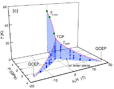
Figure 1: Observed phase diagram of UGe₂ in the space spanned by temperature ($T$), pressure ($P$) and magnetic field ($H$). Solid red curves represent lines of second-order transitions, blue planes represent first-order transitions. Also shown are the tricritical point (TCP), and the extrapolated “quantum critical end points” (QCEP)${}^{\ref{CEP_footnote}}$ at the wing tips. From Kotegawa et al. (2011b).

Strongly disordered materials, on the other hand, almost always show a continuous transition, also in agreement with the theoretical prediction. There are, however, exceptions from these general patterns, which we will discuss in Sec. II.3.1.

These predictions and observations are for systems where the transition is to a homogeneous ferromagnetic state; the schematic phase diagrams for the discontinuous and continuous cases, respectively, are shown in Fig. 2 a) and b). In other materials, magnetic order of a different kind is found to compete with homogeneous ferromagnetism at low temperatures, as schematically illustrated in Fig. 2 c). In strongly disordered systems, spin-glass freezing and quantum Griffiths effects may occur at low temperatures and augment or compete with critical behavior, see Fig. 2 d). These effects will be discussed in detail in Secs. II.4, II.5 and III.4, III.5.

The striking difference between the predictions of BKV and Hertz theory is due to a coupling of the order-parameter fluctuations to electronic degrees of freedom. Hertz theory treats this coupling in too simple an approximation to capture all of its qualitative effects. In metals at $T=0$ there are soft or gapless two-fermion excitations that couple to the magnetic order-parameter fluctuations in important ways. In effect, the combined fermionic and bosonic (order-parameter) fluctuations determine the quantum universality class in all spatial dimensions $d<3$. As a result of this coupling, the upper critical dimension is $d_{\text{c}}^{+}=3$, rather than $d_{\text{c}}^{+}=1$ as predicted by Hertz theory, and the transition is first order, rather than continuous with mean-field exponents. The mechanism behind this phenomenon is similar to what is known as a fluctuation-induced first-order transition in classical phase transitions Halperin et al. (1974); Chen et al. (1978), but it is different in at least one crucial way, cf. Secs. III.2.2 and IV.1. Two well-known classical examples of a fluctuation-induced first-order transition are the superconducting (BCS) transition, and the nematic-to-smectic-A transition in liquid crystals. In these cases, soft fluctuations of the electromagnetic vector potential (in superconductors) or the nematic order parameter (in liquid crystals) couple to the order parameter and lead to a cubic term in the equation of state, which in turn leads to a discontinuous phase transition. As we will discuss in Sec. IV, this type of mechanism is even more important and efficient in the quantum case.

We add some remarks about the relative strength of fluctuations at second-order and certain first-order transitions. At a second-order transition above the upper critical dimension, treating the fluctuations in a Gaussian approximation suffices to obtain the exact critical behavior; this is what Hertz theory concluded for the ferromagnetic QPT. At a critical point below the upper critical dimension this is not true; fluctuations are strong enough to modify the critical exponents, although they do not change the continuous nature of the transition. At a fluctuation-induced first-order transition, the combined effects of order-parameter fluctuations and other soft modes are so strong that they change the order of the transition predicted by mean-field theory. The prediction of BKV was that this will happen at the ferromagnetic QPT in clean systems.

The continuous quantum ferromagnetic transition in disordered metals, in systems where the disorder is strong enough to suppress the tricritical temperature to zero, has also been studied in detail theoretically Kirkpatrick and Belitz (1996); Belitz et al. (2001a, b). In this case the itinerant electrons are moving diffusively, rather than ballistically. Because this is a slower process, there is an effective diffusive enhancement of the exchange interaction that causes ferromagnetism, and some crucial signs in the theory are changed compared to the clean case. The net result is that the second-order transition predicted by Hertz theory becomes, so to speak, even more continuous by the coupling to the electronic soft modes: For example, the theory predicts that in $d=3$ the critical exponent $\beta$ is equal to $2$, compared to $\beta=1/2$ in Hertz theory. This large value of $\beta$ may give the impression of a “smeared transition”, even though there still is a sharp critical point. This, as well as the predicted values of other exponents, is consistent with numerous experiments in disordered systems, as we will discuss. In related developments, much work has been done on Griffiths singularities and Griffiths phases in disordered metallic magnets. Depending on the nature and symmetry of the order parameter, these theories predict that in some systems the Griffiths-phase effects are very weak, while in others they lead to strong power-law singularities with continuously varying exponents, and in yet others they completely destroy the sharp quantum phase transition (for a review, see Vojta, 2010). If these effects are important, they will be superimposed on the critical behavior.

Finally, there are theories that suggest that in some metallic systems an inhomogeneous magnetic phase may form in between the paramagnetic and the homogeneous ferromagnetic state at low $T$. This was first suggested by Belitz et al. (1997), and has been explored in detail by others. Spiral phases, spin nematics, and spin-density waves have been proposed to appear between the uniform ferromagnet and the paramagnetic phase Chubukov et al. (2004); Rech et al. (2006); Maslov et al. (2006); Efremov et al. (2008); Chubukov and Maslov (2009); Conduit et al. (2009); Karahasanovic et al. (2012). We will discuss these and related theories in Sec. III.5.

II Experimental results

In this section we discuss experimental results on quantum ferromagnets, organized with respect to the observed structures of the phase diagram as shown in Fig. 2.

II.1 General remarks

During the last two decades a large number of ferromagnetic (FM) metals have been found that (1) have a low Curie temperature, and (2) can be driven across a ferromagnet-to-paramagnet quantum phase transition. The control parameter is often either hydrostatic pressure or uniaxial stress, but the transition can also be triggered by composition, or an external magnetic field. The initial motivation for many of these experiments was to look for a ferromagnetic quantum critical point (QCP), and possibly novel states of matter in its vicinity, as had been found in many antiferromagnetic (AFM) metals Grosche et al. (1996); Mathur et al. (1998); Gegenwart et al. (2008); von Löhneysen et al. (2007); Park et al. (2006). It soon became clear, however, that the FM case is quite different from the AFM one. Instead of displaying a quantum critical point, many systems were found to undergo a first-order quantum phase transition, with a tricritical point in the phase diagram separating a line of second-order transitions at relatively high temperatures from a line of first-order transitions at low temperatures. In several of these materials the existence of a tricritical point has been confirmed by the observation of tricritical wings upon the application of an external magnetic field $H$, as shown schematically in Fig. 2 a. Some systems, such as ZrZn₂, were initially reported to have a QCP, but with increasing sample quality the transition at low temperatures was found to be first order. The first-order transition occurs across a large variety of materials, including transition metals in which the magnetism is due to $3d$ electrons, as well as $4f$- and $5f$-electron systems, see Tables 1, 2.

Figure 2: (Color online) Schematic phase diagrams observed in ferromagnetic (FM) systems that show, at the lowest temperatures realized, a) a discontinuous transition and tricritical wings in a magnetic field, b) a continuous transition, c) a change to spin-density-wave (SDW) or antiferromagnetic (AFM) order, d) a continuous transition in strongly disordered systems that may be accompanied by quantum Griffiths effects or spin-glass freezing in the tail of the phase diagram.

Some systems do show a continuous quantum phase transition to the lowest temperatures observed, see Tables 3, 4, 5 and Fig. 2 b. Several of these are either strongly disordered, as judged by their residual resistivities, or their crystal structure makes them quasi-one-dimensional. Finally, the expectation of additional phases was borne out. In some systems the long-range order changes from ferromagnetic to modulated spin-density-wave (SDW) or AFM order, see Fig. 2 c), and strongly disordered systems often show a spin-glass-like phase in the tail of the phase diagram, Fig. 2 d). Accordingly, we distinguish four categories of metallic quantum ferromagnets, namely: (1) Systems that display a first-order quantum phase transition; (2) systems that display, or are suspected to display, a quantum critical point; (3) systems that undergo a phase transition to a different type of magnetic order before the FM quantum phase transition is reached; and (4) systems with spin-glass-like characteristics or other manifestations of strong disorder at very low temperatures. This phenomenological classification, which is independent of the microscopical origin of the magnetism, is reflected in Fig. 2 and Tabs. 1–7. For each of these categories we discuss a number of representative materials in which the QPT has been reasonably well characterized. This list of materials is not exhaustive.

We also mention that superconductivity has been found to coexist with itinerant ferromagnetism in four U-based FM metals: UGe₂ (Saxena et al. (2000)), URhGe (Aoki et al. (2001); Yelland et al. (2011)), UCoGe (Huy et al. (2007a)), and UIr (Kobayashi et al. (2006)). While very interesting, this topic is outside the scope of this review and will be mentioned only in passing. Another very interesting class of materials that we do not cover are ferromagnetic semiconductors which have recently been reviewed by Jungwirth et al. (2006).

II.2 Systems showing a discontinuous transition

We first discuss systems in which there is strong evidence for a first-order transition at low temperatures. These include the transition-metal compounds MnSi and ZrZn₂, several uranium-based compounds, and some other materials; their properties are summarized in Tables 1, 2. The wide spread pattern of 1st order transitions near the QPT is consistent with fundamental arguments such as the BKV theory Belitz et al. (1999, 2005a), which for clean ferromagnets predicted a first-order quantum phase transition at $T=0$, a tricritical point in the phase diagram, and associated tricritical wings in an external magnetic field. This theory will be reviewed in Sec. III, where we will give a detailed discussion of the relation between theory and experiment.

Table 1: Systems showing a first-order transition I: Transition-metal and uranium-based compounds. FM = ferromagnetism, SC = superconductivity. $T_{\textrm{C}}$ = Curie temperature, $T_{\text{tc}}=$ tricritical temperature. $\rho_{0}=$ residual resistivity. n.a. = not available

System	Order of	$T_{\textrm{C}}$/K$\,{}^{b}$	magnetic	tuning	$T_{\text{tc}}$/K	wings	Disorder$\,{}^{d}$	Comments
	Transition$\,{}^{a}$		moment/$\mu_{\text{B}}^{c}$	parameter		observed	($\rho_{0}/\mu\Omega$cm)
MnSi	1st$\,{}^{1,2}$	$29.5\,^{3}$	$0.4\,^{3}$	pressure$\,{}^{1}$	$\approx 10\,^{1,e}$	yes$\,{}^{4}$	$0.33\,^{4}$	weak helimagnet$\,{}^{5,6}$
ZrZn2	1st$\,{}^{7}$	$28.5\,^{7}$	$0.17\,^{7}$	pressure$\,{}^{7}$	$\approx 5\,^{7}$	yes$\,{}^{7}$	$\geq 0.31\,^{8}$	long history$\,{}^{9}$
CoS2	1st$\,{}^{10,11}$	$122\,^{10}$	$0.84\,^{12}$	pressure$\,{}^{10}$	$\approx 118\,^{10}$	(yes)$\,{}^{f}$	$0.2$ – $0.6\,^{13}$	high $T_{\textrm{C}}$ and $T_{\text{tc}}$
Ni3Al	(1st?)$\,{}^{g}$	41 – 15$\,{}^{h}$	0.075$\,{}^{i}$	pressure$\,{}^{14}$	n.a.	no	0.84$\,{}^{15}$	1st order trans-
								ition suspected
UGe2	1st 16,17	$52^{\,18}$	$1.5^{\,18}$	pressure$\,{}^{18,19}$	$24\,^{20}$	yes$\,{}^{18,20}$	$0.2\,^{19}$	easy-axis FM
								coex. FM+SC$\,{}^{19}$
U3P4	1st 21	138 22	1.34 23,j	pressure 21	32 21	yes$\,{}^{21,k}$	4 21,l	canted easy-axis FM
URhGe	1st$\,{}^{17,24}$	$9.5^{\,25}$	$0.42\,^{25}$	$\perp B$-field$\,{}^{24,26}$	$\approx 1\,^{24}$	yes$\,{}^{24}$	$8\,^{27}$	easy-plane FM
								coex. FM+SC$\,{}^{25}$
UCoGe	1st$\,{}^{17,28}$	$2.5\,^{28}$	$0.03\,^{29}$	none	$>2.5\,?$ m	no	$12\,^{29}$	very weak FM
								coex. FM+SC$\,{}^{29}$
UCoAl	1st$\,{}^{30,n}$	$\approx 0\,^{30,31,o}$	$0\,^{30,31,o}$	pressure$\,{}^{30,31}$	$>11$ K$\,{}^{30}$	yes$\,{}^{30}$	24$\,{}^{30}$	easy-axis FM
URhAl	1st$\,{}^{33}$	$34$ – $25\,^{32,33}$	$\approx 0.9\,^{32,33}$	pressure$\,{}^{33}$	$\approx 11\,^{33}$	yes$\,{}^{33}$	$\approx$ 65$\,{}^{33}$	weakly 1st order
a At the lowest temperature achieved.
b A single value of $T_{\textrm{C}}$ at the default value of the tuning parameter (ambient pressure, zero field) is given if $T_{\text{tc}}$ has also been
measured; a range of $T_{\textrm{C}}$ for a range of control parameters in all other cases.  c Per formula unit unless otherwise noted.
d For the highest-quality samples. e Disputed by Stishov et al. (2007); see text.
f Metamagnetic behavior in 1st-order region indicative of wings.
g Suspected 1st order transition near $p=80$ kbar Niklowitz et al. (2005); Pfleiderer (2007).
h For pressures $p=0$ – $60$ kbar. i Per Ni at $p=0$ Niklowitz et al. (2005). j Per U.
k Via a metamagnetic transition; wings have not been mapped out. l At the critical pressure $p_{c}\approx 4$ GPa.
m Pressure decreases $T_{\textrm{C}}$ Slooten et al. (2009); TCP not accessible. $T_{\textrm{C}}$ increases nonmonotonically upon doping with Rh
Sakarya et al. (2008); order of transition for URhxCo1-xGe not known except for $x=1$ (2nd order with $T_{\textrm{C}}$ = 9.5 K).
n Inferred from existence of tricritical wings.
o PM at zero pressure. Uniaxial pressure induces FM, so does doping, see Ishii et al. (2003) and references therein.
1 Pfleiderer et al. (1997)		2 Uemura et al. (2007)			3 Ishikawa et al. (1985)			4 Pfleiderer et al. (2001a)
5 Ishikawa et al. (1976)		6 Mühlbauer et al. (2009)			7 Uhlarz et al. (2004)			8 Sutherland et al. (2012)
9 Pfleiderer (2007)		10 Goto et al. (1997)			11 Goto et al. (2001)			12 Adachi et al. (1969)
13 Sidorov et al. (2011a)		14 Niklowitz et al. (2005)			15 Steiner et al. (2003)			16 Huxley et al. (2001)
17 Aoki et al. (2011b)		18 Kotegawa et al. (2011b)			19 Saxena et al. (2000)			20 Taufour et al. (2010)
21 Araki et al. (2015)		22 Trzebiatowski and Troć (1963)			23 Wiśniewski et al. (1999)			24 Huxley et al. (2007)
25 Aoki et al. (2001)		26 Levy et al. (2005)			27 Miyake et al. (2009)			28 Hattori et al. (2010)
29 Huy et al. (2007b)		30 Aoki et al. (2011a)			31 Ishii et al. (2003)			32 Veenhuizen et al. (1988)
33 Shimizu et al. (2015b)

Table 2: Systems showing a first-order transition II: Lanthanide-based compounds, and strontium ruthenates. $T_{\textrm{C}}$ = Curie temperature, $T_{\text{tc}}=$ tricritical temperature. $\rho_{0}=$ residual resistivity. n.a. = not available.

System	Order of	$T_{\textrm{C}}$/K	magnetic	tuning	$T_{\text{tc}}$/K	wings	Disorder$\,{}^{c}$	Comments
	Transition$\,{}^{a}$		moment/$\mu_{\text{B}}\,^{b}$	parameter		observed	($\rho_{0}/\mu\Omega$cm)
La1-xCexIn2	1st$\,{}^{1}$	22 – 19.5 $\,{}^{1,d}$	n.a.	composition$\,{}^{1}$	$>22$ ?$\,{}^{e}$	no	n.a.	third phase?$\,{}^{1}$
SmNiC2	1st$\,{}^{2}$	17 – 15$\,{}^{2,f}$	0.32$\,{}^{2}$	pressure$\,{}^{2}$	$>17$ ?	no	2	other phases$\,{}^{2}$
YbCu2Si2	1st$\,{}^{3}$	4.7 – 3.5$\,{}^{3,2,g}$	0.16 – 0.42$\,{}^{3,h}$	pressure$\,{}^{3-5}$	n.a.	no	$<$ 0.5$\,{}^{6}$	strong Ising
								anisotropy$\,{}^{3}$
YbIr2Si2	1st$\,{}^{7}$	2.3 – 1.3$\,{}^{i}$	n.a.	pressure$\,{}^{7}$	n.a.	no	$\approx 22$ j	FM order
								suspected$\,{}^{7}$
CePt	(1st?)$\,{}^{8}$	5.8 – 0$\,{}^{9,8}$	n.a.	pressure$\,{}^{8}$	n.a.	no	$\approx$ 11$\,{}^{9}$	1st order trans-
								ition suspected
Sr1-xCaxRuO3	1st$\,{}^{10}$	160 – 0$\,{}^{k}$	0.8 – 0$\,{}^{k}$	composition$\,{}^{10}$	n.a.	no	n.a.	ceramic samples
Sr3Ru2O7	1st$\,{}^{l}$	0$\,{}^{m}$	0$\,{}^{m}$	pressure$\,{}^{m}$	n.a.	yes 11	$<0.5$$\,{}^{11}$	foliated wings,
								exotic phase$\,{}^{11}$
a At the lowest temperature achieved. b Per formula unit unless otherwise noted. c For the highest-quality samples.
d For $x=1.0$ – $0.9$. e 1st order for $x=1$, TCP not accessible. f For $p=0$ – 2 GPa. g For pressures $p\approx 11.5$ – $9.4$ GPa.
h For pressures $p=9.4$ – $11.5$ GPa. i For pressures $p\approx 10$ – $8$ GPa.
j For a magnetic sample at pressures $p\approx 8$ – $10$ GPa. Samples with $\rho_{0}$ as low as 0.3$\mu\Omega$cm at ambient pressure have been
prepared Yuan et al. (2006). k For $x=0$ to $x\gtrsim 0.7$.
l Phase diagram not mapped out completely; the most detailed measurements show tips of wings. See Wu et al. (2011).
m Paramagnetic at ambient pressure. Hydrostatic pressure drives the system away from FM, uniaxial stress drives it towards
FM. See Wu et al. (2011) and references therein, especially Ikeda et al. (2000).
1 Rojas et al. (2011)			2 Woo et al. (2013)		3 Tateiwa et al. (2014)		4 Winkelmann et al. (1999)
5 Fernandez-Pañella et al. (2011)			6 Colombier et al. (2009)		7 Yuan et al. (2006)		8 Larrea et al. (2005)
9 Holt et al. (1981)			10 Uemura et al. (2007)		11 Wu et al. (2011)

II.2.1 Transition-metal compounds

MnSi

MnSi is a very well-studied material in which the search for a FM QCP resulted in the observation of a first-order quantum phase transition. The transition temperature at ambient pressure is $T_{\textrm{C}}$  $\approx 29.5\,$K, and the application of hydrostatic pressure suppresses $T_{\textrm{C}}$ to zero at a critical pressure $p_{c}\approx 14.6\,$kbar Pfleiderer et al. (1994, 1997). This compound is actually a weak helimagnet Ishikawa et al. (1976), due to its B21 crystal structure that lacks inversion symmetry, with a complicated phase diagram (see Mühlbauer et al., 2009 and references therein). However, the long wavelength of the helix, about 180 Å, allows one to approximate the system as a ferromagnet. The helical order implies that the transition should be very weakly first order even at ambient pressure Bak and Jensen (1980). This has indeed been observed Stishov et al. (2007, 2008); Janoschek et al. (2013). Pfleiderer et al. (1997) found evidence of a strongly first-order transition for pressures $p^{*}<p<p_{c}$ with $p^{*}\approx 12\ \text{kbar}$. The tricritical temperature (i.e., the transition temperature at $p=p^{*}$) is $T_{\text{tc}}\approx 12\,$K. These results were later corroborated by the observation of tricritical wings (Pfleiderer et al., 2001a, the observed phase diagram is shown in Fig. 3), and by $\mu$SR data that show, for $p^{*}<p<p_{c}$, phase separation indicative of a first-order transition Uemura et al. (2007), see Fig. 4. Moreover, this has been confirmed by neutron Larmor diffraction experiments under pressure Pfleiderer et al. (2007). Conversely, data presented by Stishov et al. (2007), Petrova et al. (2009), and Petrova and Stishov (2012), suggests that the quantum phase transition at $p=p_{c}$ is either continuous or very weakly first order. Although the evidence for a pressure induced first-order transition appears convincing in the purest crystals, no agreement has been reached Otero-Leal et al. (2009a); Stishov (2009); Otero-Leal et al. (2009b).

Figure 3: Phase diagram of MnSi. In the temperature - pressure ($T$-$p$) plane the transition temperature drops from $T_{\textrm{C}}$ $=29.5\,$K at ambient pressure and changes from second to first order at $p^{*}=12\,$kbar where $T_{\textrm{C}}$ $\approx 12\,$K. $T_{\textrm{C}}$ vanishes at $p_{\text{c}}=14.6$ kbar. In the magnetic field - pressure ($B$-$p$) plane at $T=0$, and everywhere across the shaded wing, the transition is first order up to a “critical endpoint”${}^{\ref{CEP_footnote}}$ estimated to be located at $B_{\text{m}}=0.6\,$T and $p_{\text{m}}=17\,$kbar. From Pfleiderer et al. (2001a).

Figure 4: $\mu$SR results for the volume fraction with static magnetic order. The nonzero volume fraction less then unity at $T=0$ for intermediate pressures indicates phase separation, which in turn is indicative of a first-order transition. From Uemura et al. (2007).

For $p<p_{c}$ the properties of MnSi are in good semiquantitative agreement with the SCR theory Pfleiderer et al. (1997). Specifically, $T^{4/3}_{\textrm{C}}$ is a linear function of the pressure. This agreement fails at $p\rightarrow p_{c}$ due to the presence of the first-order transition. Also, a striking $T^{3/2}$ power law for the resistivity was observed in a broad range of $p\gtrsim p_{c}$ Pfleiderer et al. (2001b) where we would expect a Fermi-liquid $T^{2}$ behavior. The nature of this power law in resistivity, which seems to be a common feature in itinerant magnets near their QPT (cf. Sec. IV.2), is still unclear.

ZrZn₂

Another transition-metal compound with very similar behavior across the quantum ferromagnetic transition, but without the complications resulting from helical order, is ZrZn₂. It crystallizes in the cubic C15 structure and is a true ferromagnet Matthias and Bozorth (1958); Pickart et al. (1964) with a small magnetic anisotropy and an ordered moment of $0.17\,$$\mu_{\textrm{B}}$  per formula unit Uhlarz et al. (2004). The material can be tuned across the transition by means of hydrostatic pressure. While early experiments Smith et al. (1971); Huber et al. (1975); Grosche et al. (1995) suggested the existence of a quantum critical point, an increase in sample quality led to the realization that the transition becomes first order at high $p$, causing a first-order quantum phase transition with a critical pressure $p_{c}\approx 16.5\,$kbar Uhlarz et al. (2004). The transition temperature at ambient pressure is $T_{\textrm{C}}$ $\approx 28.5\,$K, and the tricritical temperature is $T_{\text{tc}}\approx 5\,$K. The phase diagram is qualitatively the same as that shown in Fig. 3; the observation of tricritical wings by Uhlarz et al. (2004) confirmed an earlier suggestion by Kimura et al. (2004). The first-order nature of the QPT was confirmed by Kabeya et al. (2012, 2013), who also studied crossover phenomena above the tricritical wings. However, the transition is weakly first order and, for $p<p_{c}$, ZrZn₂ can be reasonably well undestood within the SCR theory Grosche et al. (1995); Smith et al. (2008). Surprisingly, the resistivity exponent shows an abrupt change from 5/3 for $p<p_{c}$ to 3/2 at $p>p_{c}$ and remains 3/2 up to higher pressures (about 25 kbar), similarly to MnSi. In ZrZn₂ as well as in other itinerant magnets such a NFL behavior is still not understood (cf. Sec. IV.2).

CoS₂

Cobalt disulphide crystallizes in a cubic pyrite structure. It is an itinerant ferromagnet with $T_{\textrm{C}}$ $\approx 124$ K, an ordered moment of 0.84 $\mu_{\textrm{B}}$/Co, and an effective moment of 1.76 $\mu_{\textrm{B}}$/Co Jarrett et al. (1968); Adachi et al. (1969). Density-functional calculations concluded that CoS₂ is a half-metallic ferromagnet Zhao et al. (1993); Mazin (2000). The spin polarization is high at about 56% Wang et al. (2004), and the transport coefficients and the thermal expansion coefficient show unusual behavior in the vicinity of the transition Adachi and Ohkohchi (1980); Yomo (1979). Magnetization measurements indicate that the transition is almost first order at ambient pressure Wang et al. (2004). Hydrostatic pressure decreases $T_{\textrm{C}}$, and at a pressure of about 0.4 GPa the nature of the transition changes from second order to first order, with a tricritical temperature $T_{\text{tc}}\approx 118\,$K Goto et al. (1997). A much lower value for the tricritical pressure was found by Otero-Leal et al. (2008); however, this analysis depended on a specific model equation of state. Sidorov et al. (2011a) confirmed a strongly first order QPT at a critical pressure of about 4.8 GPa. $T_{\textrm{C}}$  is also suppressed if selenium is substituted for sulphur, and the transition again becomes first order at a small selenium concentration, with 1% of selenium roughly equivalent to a pressure of 1 GPa Hiraka and Endoh (1996).

Two groups have investigated the $p\,$-$T$ phase diagram at higher pressures up to the QPT: Barakat et al. (2005) observed a monotonically decreasing $T_{\textrm{C}}$  with increasing pressure. They inferred a first-order quantum phase transition at $p_{\text{c}}\approx 6$ GPa from a change of the temperature dependence of the resistivity ($\rho(T)=\rho_{0}+AT^{n}$) from $n=2$ in the FM phase to $n\approx 1.6$ for $p>p_{\text{c}}$. Their samples had a residual resistivity $\rho_{0}\approx 2\,\mu\Omega$cm and a residual resistance ratio (RRR) of about 60. Sidorov et al. (2011a) performed experiments on a better sample ($\rho_{0}\approx 0.7\,\mu\Omega$cm) and concluded that $p_{\text{c}}=4.8$ GPa. They found that the temperature dependence of the resistivity does not change across the transition, with $n=2$ both below and above $p_{\text{c}}$, while the residual resistivity drops by about a factor of 3 as the transition is crossed.

These discrepancies notwithstanding, all experiments agree on the first-order nature of the quantum phase transition. This makes the phase diagrams of CoS₂, ZrZn₂, and MnSi qualitatively the same. It is worthwhile noting that the tricritical temperatures correlate with the size of the ordered moment, with the largest moment corresponding to the highest $T_{\text{tc}}$.

Ni₃Al

Ni₃Al crystallizes in the simple cubic Cu₃Au structure. Its magnetic properties depend on the exact composition; the stoichiometric compound at ambient pressure is a ferromagnet with a Curie temperature $T_{\textrm{C}}$ = 41 K and a small ordered moment of 0.075 $\mu_{\text{B}}$/Ni de Boer et al. (1969); Niklowitz et al. (2005). $T_{\textrm{C}}$  decreases upon the application of hydrostatic pressure and vanishes at a critical pressure of 8.1 GPa Niklowitz et al. (2005). The resistivity of stoichiometric Ni₃Al shows a pronounced non-Fermi-liquid (NFL) temperature dependence on either side of the transition, $\Delta\rho\propto T^{n}$, with $n$ somewhere between 3/2 and 5/3 Fluitman et al. (1973); Steiner et al. (2003); Pfleiderer (2007). At ambient pressure and in zero magnetic field Steiner et al. (2003) found $n=1.65$ for temperatures between about 0.5 and 3.5 K. The prefactor is comparable with that of the $T^{3/2}$ behavior of the resistivity in ZrZn₂ Pfleiderer et al. (2001b); Yelland et al. (2005).

The transition at ambient pressure is second order, and the overall form of the phase diagram is consistent with the results of the spin-fluctuation theory described in Sec. III.3.2, as is the logarithmic temperature dependence of the specific heat Sato (1975); Yang et al. (2011); Niklowitz et al. (2005). However, studies of the temperature dependence of the resistivity under pressure suggest that the quantum phase transition at the critical pressure is first order Niklowitz et al. (2005); Pfleiderer (2007). This would be analogous to the behavior of MnSi, Sec. II.2.1, where overall behavior consistent with spin-fluctuation theory also gives way to a first-order transition at low temperatures. Since the magnetic moment in Ni₃Al is smaller than in MnSi, the theory discussed in Sec. III.2.2 predicts the tricritical temperature in the former to be lower than in the latter, see the discussion in Sec. II.2.5, which is consistent with the experimental evidence.

$T_{\textrm{C}}$ also decreases upon doing of Ni₃Al with Pd Sato (1975) or Ga Yang et al. (2011); these systems are discussed in Sec. II.3.1.

II.2.2 Uranium-based compounds

Ferromagnetism with a first-order transition at low transition temperatures has been observed in the uranium-based heavy-fermion compounds UGe₂ Huxley et al. (2000); Taufour et al. (2010); Kotegawa et al. (2011b), URhGe Huxley et al. (2007), and UCoGe Hattori et al. (2010). UCoAl is paramagnetic at ambient pressure, but very close to a first-order quantum phase transition Aoki et al. (2011a). The ferromagnetism is due to $5f$ electrons. The extent to which these electrons are localized or itinerant, and the consequences for neutron-scattering observations, have been investigated in some detail Yaouanc et al. (2002); Fujimori et al. (2012); Chubukov et al. (2014). Coexistence of ferromagnetism and superconductivity (SC) has been found in UGe₂ Saxena et al. (2000); Huxley et al. (2001), URhGe Aoki et al. (2001), and UCoGe Huy et al. (2007b); for a recent overview, see Aoki and Flouquet (2014).

UGe₂

UGe₂ has received much attention since superconductivity coexists with ferromagnetism in part of the ordered phase Saxena et al. (2000). It crystallizes in an inversion-symmetric orthorhombic structure, and the best samples have been reported to have residual resistivities as low as $0.2\,\mu\Omega$cm Saxena et al. (2000). Taufour et al. (2010) found the residual resistivity to be strongly pressure dependent. The Curie temperature at ambient pressure is $T_{\textrm{C}}$ $\approx 52\,$K Saxena et al. (2000); Huxley et al. (2001); Aoki et al. (2001); Aoki and Flouquet (2012). $T_{\textrm{C}}$ decreases with increasing hydrostatic pressure and vanishes at $p\approx 16$ kbar, which coincides with the pressure where the superconductivity disappears. Within the ferromagnetic phase a further transition is observed, across which the magnitude of the magnetic moment changes discontinuously. The associated transition line starts near the peak in the superconducting transition temperature, ends in a critical point at a temperature of about 4 K, and is replaced by a crossover at higher temperatures Huxley et al. (2007); Taufour et al. (2010), see Fig. 5.

Figure 5: Phase diagram of UGe₂ in the temperature-pressure plane. Shown are the paramagnetic (PM) phase, two ferromagnetic phases (FM1 and FM2), and the tricritical point (TCP). The critical point marked CEP ${}^{\ref{CEP_footnote}}$ is related to the transition between the phases FM1 and FM2. From Taufour et al. (2010).

The tricritical temperature has been measured to be $T_{\text{tc}}\approx 24\,$K Taufour et al. (2010); Kotegawa et al. (2011b), but values as high as $T_{\text{tc}}\approx 31\,$K have been reported Huxley et al. (2007) with a tricritical pressure $p_{\text{tc}}\approx 13$ kbar. Kabeya et al. (2010) found a somewhat smaller value of $\approx 12.5$ kbar from measurements of the linear thermal expansion coefficient. The tricritical wings have been mapped out in detail, see Fig. 1.

U₃P₄

U₃P₄ at ambient pressure is a ferromagnet with $T_{\textrm{C}}$ = 138 K Trzebiatowski and Troć (1963). It crystallizes in a bcc structure with no inversion symmetry, and the magnetic structure is canted with a FM component along $\langle 111\rangle$ Burlet et al. (1981); Wiśniewski et al. (1999); Heimbrecht et al. (1941); Zumbusch (1941). Pressure reduces $T_{\textrm{C}}$ until a QPT is reached at $p_{\text{c}}\approx 4\,$GPa. From measurements of the resistivity and the magnetic susceptibility at $p\approx 1.5\,$GPa, Araki et al. (2015) concluded that the transition changes from second order to first order with a tricritical temperature $T_{\text{tc}}=32\,$K. Consistent with this, the pressure-dependence of $T_{\textrm{C}}$ changes from a Hertz-type $T_{\textrm{C}}$ $\propto(p-p_{\text{c}})^{3/4}$ behavior to $T_{\textrm{C}}$ $\propto(p-p_{\text{c}})^{1/2}$. In a magnetic field, metamagnetic behavior has been observed that is indicative of tricritical wings, although the wings have not been mapped out.

URhGe and UCoGe

Both of these materials belong to the ternary UTX intermetallic U-compounds where T is one of the late transition metals and X a $p$-electron element. They crystallize in the orthorhombic TiNiSi structure (space group $P_{nma}$). For lattice parameters, see Troć and H.Tran (1988) and Canepa et al. (2008). Because the $5f$-electrons, which carry the magnetic moments, are partially delocalized in these materials, the ordered moment is often reduced compared to the free ion value and an enhanced electronic specific heat is observed. In addition, they are characterized by a strong Ising anisotropy Sechovsky and Havela (1998). Two main mechanisms control the delocalization of the $5f$ electrons and thus the magnetism: the direct overlap of neighbouring U $5f$ orbitals and the hybridization of those with the $d$-electrons. For inter-U distances smaller than the so-called Hill limit ($d_{U-U}\approx 3.4-3.6$ Å) Hill (1970) the strong direct overlap of the $5f$ orbitals results in a non-magnetic ground state. Larger values yield a FM or AFM ordered ground state. For values close to this limit the $f-d$ hybridization strength controls the magnetic properties. There is a clear tendency of these systems to show magnetic order with increasing $d$-electron filling of the T element Sechovsky and Havela (1998). The strongest electronic correlations are therefore found in UTX compounds with intermediate values of $d_{U-U}$ and $d$-electron filling.

Figure 6: Phase diagram of URhGe in the space spanned by temperature and magnetic fields in the b- and c-directions. The dark shaded regions indicate the presence of superconductivity. From Huxley et al. (2007).

URhGe has a $d_{U-U}=3.5$ Å close to the Hill limit. It is ferromagnetic with a Curie temperature $T_{\textrm{C}}$ $=9.5\,$K and an ordered moment of 0.42 $\mu_{\textrm{B}}$, oriented along the c-axis. It was the second U-based compound (after UGe₂) for which coexistence of superconductivity and ferromagnetism was found in high-quality samples Aoki et al. (2001). It is unique in that a magnetic field parallel to the b-axis suppresses $T_{\textrm{C}}$ and leads to a tricritical point at $T\approx 1\,$K and $H_{b}\approx 12\,$T Huxley et al. (2007). With an additional field in the c-direction, tricritical wings appear, see Fig. 6. The superconductivity is absent at intermediate fields, but reappears at low temperatures in the vicinity of the tricritical wings Levy et al. (2005); Huxley et al. (2007).

Figure 7: Phase diagram of UCoGe in the temperature-pressure plane, showing the ferromagnetic and superconducting phases. The magnetic transition is first order for all pressure values Hattori et al. (2010). After Slooten et al. (2009).

Figure 8: Curie temperature of URhGe doped with Co, Si, or Rh as a function of the dopant concentration. The transition in pure URhGe is 2nd order, in pure UCoGe, 1st order. From Sakarya et al. (2008).

The nature of the magnetic order in UCoGe, ferromagnetic or otherwise, was initially unclear. This, together with the observation that URhGe is ferromagnetic, prompted the study of URh_1-xCo_xGe alloys Sakarya et al. (2008), and the final conclusion was that UCoGe is indeed a weak ferromagnet with a Curie temperature near 3 K and a small ordered moment of 0.03 $\mu_{\textrm{B}}$ Huy et al. (2007b). The transition was found to be weakly first order by means of nuclear quadrupole resonance measurements Hattori et al. (2010). Hydrostatic pressure decreases $T_{\textrm{C}}$ Hassinger et al. (2008); Slooten et al. (2009) which vanishes near the maximum of the superconducting dome, see Fig. 7. A tricritical point must appear as $T_{\textrm{C}}$ increases upon doping with Rh, see Fig. 8, but the order of the transition has not been studied as a function of the Rh concentration. Similarly, in pure UCoGe tricritical wings should appear in a magnetic field, analogously to what is observed in UCoAl, see Fig. 10. A recent study has reported that $T_{\textrm{C}}$ is suppressed by doping with Ru, with an extrapolated critical Ru concentration of about 31% Vališka et al. (2015). The order of the transition has not been determined.

UCoGe displays coexistence of superconductivity and ferromagnetism below 0.8 K Huy et al. (2007b); Slooten et al. (2009). In contrast to both UGe₂ and URhGe the superconductivity is observed in both the ferromagnetic and paramagnetic phases, see Fig. 7.

UCoAl

Figure 9: a) Magnetostriction measured along the $c$-axis with $H\parallel c$ for temperatures between 2 and 21 K (every 1 K). b) Temperature vs field evolution of the metamagnetic transition which changes from first order to a crossover for $T>T_{0}=11$ K. From Aoki et al. (2011a).

At ambient pressure and zero field, UCoAl is a paramagnet with a strong uniaxial magnetic anisotropy Sechovsky et al. (1986). It crystallizes in the hexagonal ZrNiAl structure consisting of U-Co and Co-Al layers that alternate along the c-axis. The inter-U distance is $d_{U-U}\approx 3.5$ Å (same value as in URhGe, see II.2.2), but a large $d$-filling leads to UCoAl being paramagnetic Sechovsky and Havela (1998). Its isoelectronic analog URhAl is ferromagnetic with $d_{U-U}\approx 3.63$ Å, (cf. Sec. II.2.2). These observations suggest that UCoAl is close to a FM instability, which is indeed the case: Application of a magnetic field along the easy magnetization axis (the crystallographic $c$-axis) induces a first-order metamagnetic phase transition at $H_{m}\approx 0.7$ T at low temperature with an induced moment of about 0.3 $\mu_{\textrm{B}}$ Andreev et al. (1985); Mushnikov et al. (1999). Moreover, uniaxial stress induces ferromagnetism Ishii et al. (2003); Shimizu et al. (2015c). The susceptibility shows Curie-Weiss behavior for $T>40$ K with a fluctuating moment of about 1.6 $\mu_{\textrm{B}}$, much larger than the induced moment of 0.3 $\mu_{\textrm{B}}$ Havela et al. (1997). The magnetism is believed to be itinerant with the U $5f$-electrons providing the main contribution Eriksson et al. (1989); Wulff et al. (1990); Mushnikov et al. (1999); polarized-neutron diffraction experiments have found the magnetic moment exclusively at the U sites with the orbital moment being twice as large as (and antiparallel to) the spin moment Wulff et al. (1990); Javorský et al. (2001).

Figure 10: Semi-schematic $T$-$P$-$H$ phase diagram with $H\parallel c$ showing the existence of tricritical wings in UCoAl. The wings are determined by the observation of a first-order metamagnetic transition at $H_{m}$ (red dots); they are bounded by lines of second-order transitions at $T_{0}$ and end in quantum “critical end points” (QCEPs)${}^{\ref{CEP_footnote}}$. The critical pressure $P_{\text{c}}$ is negative and the tricritical point (TCP) is not accessible. See the text for more information. From Aoki et al. (2011a).

Studies of the magnetostriction, magnetoresistivity Aoki et al. (2011a), nuclear magnetic resonance Karube et al. (2012) and thermopower Palacio-Morales et al. (2013) indicate that the field-induced first-order transition terminates in a critical point at a temperature $T_{0}=11$ K at ambient pressure, as illustrated in Fig. 9: $\Delta L(H)/L$ shows a step-like jump at $H_{m}$ for $T<T_{0}$ which becomes smooth for $T\geq T_{0}$. A determination of critical exponents suggests that the transition at $T_{0}$ is in the three-dimensional Ising universality class Karube et al. (2012). $H_{m}$ increases with pressure and each wing terminates in a quantum critical point (denoted by QCEP in the figure)${}^{\ref{CEP_footnote}}$ at $P\approx 1.5$ GPa and $\mu_{0}H\approx 7$ T. At the wing-tip point a pronounced enhancement of the effective mass (derived from the coefficient of the $T^{2}$ term in the electrical resistivity) is observed Aoki et al. (2011a).

The resulting $T$-$P$-$H$ semi-schematic phase diagram is shown in Fig. 10, which demonstrates the presence of tricritical wings in UCoAl. The red dots represent the experimental values for $H_{m}$ determined by magnetoresistivity (with $J\perp H$) and magnetostriction measurements. Since $T_{0}=11$ K at the ambient pressure, the tricritical point (TCP) must be located at $T>11$ K. At pressures higher than 1.5 GPa, the first-order character of the metamagnetic transition disappears and new features in the form of kinks in the magnetoresistivity and Hall effect are observed at $H_{m}$ and $H^{*}$ Combier et al. (2013). Very recent investigations of the transverse and longitudinal resistivities and of the magnetization under pressure Combier (2013) point to a much richer phase diagram, where the exact location of the QCEP remains uncertain, with possible changes of the Fermi surface as well as the appearance of new phases around the QCEP.

The substitution of Fe for Co was found to lead to FM ground state in zero field and ambient pressure by Karube et al. (2015). By nuclear quadrupole resonance measurements these authors found a first-order transition in U(Co_1-xFe_x)Al with a transition temperature of about 10 K and about 17 K for $x=0.1$ and $x=0.02$, respectively.

URhAl

URhAl belongs to the same UTX compound family as URhGe, UCoGe, and UCoAl. It has the same layered hexagonal ZrNiAl-type crystal structure as UCoAl, but with $d_{U-U}=3.63$ Å, larger than the Hill limit (cf. Sec. II.2.2).

Figure 11: Upper panel: Temperature-pressure phase diagram of URhAl in zero field determined from resistivity measurements. Lower panel: Temperature-pressure-field diagram inferred from metamagnetic behavior observed in an external field. From Shimizu et al. (2015b).

Consistent with this, and contrary to UCoAl which has a nonmagnetic ground state, URhAl orders ferromagnetically via a second-order transition. Values of the Curie temperature between $T_{\textrm{C}}$  = 27 K and $T_{\textrm{C}}$ = 34 K have been reported, with strong Ising-like ordered moments of 0.9 $\mu_{\textrm{B}}$/U along the $c$-axis Veenhuizen et al. (1988); Combier (2013); Shimizu et al. (2015b).

The itinerant vs localized nature of magnetism in URhAl is controversial, as it is in many other UTX compounds. A peak at 380 meV in inelastic neutron scattering experiments Hiess et al. (1997) was interpreted as indication of an intermultiplet transition, suggesting $5f$-electron localization. X-ray magnetic circular dichroism (XMCD) experiments also indicate a high degree of localization of the $5f$-orbitals Grange et al. (1998). On the other hand, polarized neutron studies point to a rather strong delocalization of the $5f$ electrons Paixao et al. (1992). Moreover, band structure calculations based on an itinerant approach can reproduce quite well most of the experimental findings, i.e. magneto-optical Kerr effect Kuc̆era et al. (1998), equilibrium volume, bulk modulus, magnetocrystalline anisotropy energy, magnetocrystalline anisotropy of the U moments and the shape of the XMCD lines Kuneš et al. (2001).

Pressure experiments were performed on a rather clean single crystal with a RRR $\approx 14$ and $T_{\textrm{C}}$  = 28 K Combier (2013). At ambient pressure the phase transition is mean-field-like characterized by a single peak in $C/T$ and a kink in the thermal expansion ratio $\Delta L/L$. The magnetization with $H\parallel c$ shows a clear hysteresis at 2 K with a remanent magnetization of 0.9 $\mu_{\textrm{B}}$/U. desirable. Recent transport experiments on moderately disordered samples ($\rho_{0}\approx 65\,\mu\Omega$cm near the transition) have mapped out the phase diagram in more detail Shimizu et al. (2015b, a). The QPT at a critical pressure $p_{c}\approx 5.2$ GPa is weakly first order, and metamagnetic signatures in an applied magnetic field imply the existence of tricritical wings. Due to the weakly first-order nature of the transition strong spin fluctuations are still observable in the behavior of the electrical resistivity and the specific heat.

II.2.3 Lanthanide-based compounds

La_1-xCe_xIn₂

CeIn₂ crystallizes in the orthorhombic CeCu₂ structure and undergoes a first-order transition to a ferromagnetic state at a Curie temperature $T_{\textrm{C}}$ = 22 K Rojas et al. (2009). This conclusion on the basis of discontinuities at $T_{\textrm{C}}$  in the resistivity, the thermal expansion, and the magnetic entropy was later corroborated by $\mu$SR measurements Rojas et al. (2011). Application of hydrostatic pressure increases $T_{\textrm{C}}$  Mukherjee et al. (2012), but upon doping with lanthanum $T_{\textrm{C}}$  decreases, to about 19.4 K in La_1-xCe_xIn₂ with $x=0.9$, and the transition remains first order Rojas et al. (2011). The same $\mu$SR measurements indicated the existence of a second magnetic phase with long-range order in between the FM and PM phases. The nature of this phase is not known. Doping with Ni decreases $T_{\textrm{C}}$  sharply, and the transition in Ce(In_1-xNi_x)₂ has been reported to be second order to a FM for $x=0.025$, $0.05$, and $0.15$ Rojas et al. (2013). However, an earlier experiment by Sung et al. (2009) concluded that the ground state for $x=0.15$ is AFM.

SmNiC₂

The ferromagnetic charge-density-wave (CDW) compound SmNiC₂ has a $T_{\textrm{C}}$ of about 17 K which is weakly susceptible to pressure Woo et al. (2013). The polycrystalline samples measured are rather clean, with a residual resistivity of less than 2 $\mu\Omega$cm for pressures below about 3 GPa. The PM-FM transition is first order and remains first order as the pressure is increased from zero to 2 GPa, with $T_{\textrm{C}}$ dropping to 15 K. At higher pressure, there is a second or weakly first-order transition from the FM to a phase of unclear nature, and at least two other phases appear at low temperature. Since the nonmagnetic phase in this material is a CDW state below $T\approx 150\,$K, the phase diagram may fall outside the classification provided by Fig. 2 and the first-order transition may be of different origin than in other materials, see Sec. III.6. If the theory discussed in Sec. III.2.2 applies, one expects a tricritical point at negative pressure. In this case a metamagnetic transition corresponding to the tricritical wings should be visible in an applied magnetic field, provided the zero-pressure line is not already past the wing tips.

Yb-based systems

YbCu₂Si₂ crystallizes in the body-centered ThCr₂Si₂ structure and does not order magnetically at ambient pressure. A transition to a magnetically ordered phase under pressure was suggested early on the basis of transport measurements Alami-Yadri and Jaccard (1996); Alami-Yadri et al. (1998), and later confirmed by means of Mössbauer data Winkelmann et al. (1999). Fernandez-Pañella et al. (2011) concluded from susceptibility measurements that the nature of the order is FM, and the transition is likely first order Winkelmann et al. (1999); Colombier et al. (2009); Fernandez-Pañella et al. (2011). The FM nature of the ordered phase was confirmed by Tateiwa et al. (2014), who also found evidence for phase separation indicative of a first-order transition.

YbIr₂Si₂ crystallizes in either the ThCr₂Si₂ structure, or the $P$-type CaBe₂Ge₂ structure, depending on the synthesis conditions Hossain et al. (2005). The former is magnetically (presumably AFM) ordered below 0.7 K, whereas the latter is a paramagnet at ambient pressure. Yuan et al. (2006) found that by applying pressure the system in its $P$-type structure undergoes a first-order QPT to an ordered phase at a critical pressure $p_{\text{c}}\approx 8\,$GPa. The nature of the ordered phase is suspected to be FM, but additional investigations are needed. Recent measurements of the resistivity under hydrostatic pressure as high as 15 GPa found NFL behavior in a rather broad range in pressure, $3\leq p\leq 8$ GPa, and confirmed the sudden appearence of magnetic ordering at 8.3 GPa suggestig a first-order QPT Macovei (2010). The transition temperature shifts to higher values and shows a weak maximum around 11 GPa, a behavior very similar to that of YbRh₂Si₂  under pressure Mederle et al. (2001); Knebel et al. (2006). YbRh₂Si₂  evolves from an AFM to a FM ordered state under chemical pressure (Co substitution) Lausberg et al. (2013) and possibly even under hydrostatic pressure Knebel et al. (2006). This suggests that the nature of the magnetic ordered phase in YbIr₂Si₂ could also be AFM, but more investigations are needed.

CePt

CePt under pressure has also been reported to display a ferromagnetic quantum phase transition at $p_{\textrm{c}}\approx 12.1\,$GPa Larrea et al. (2005). The phase transition at $p=0$ is second order Holt et al. (1981). No magnetization measurements have been performed under pressure. The FM signature is strongly weakened under pressure well before $p_{\textrm{c}}$ and transport experiments indicate a sudden drop of the phase boundary line close to $p_{\textrm{c}}$ suggesting the presence of a first-order transition.

II.2.4 Strontium Ruthenates

The perovskite ruthenates, which include Sr₂RuO₄ and Sr₄Ru₃O₁₀ in addition to SrRuO₃ and Sr₃Ru₂O₇, belong to a class of materials known as the Ruddlesden-Popper series; for a historical overview, see Mackenzie and Grigera (2004). In SrRuO₃ a QPT can be triggered by means of doping with Calcium, whereas the phase diagram of Sr₃Ru₂O₇ has been explored by applying pressure and an external magnetic field. In Sr_1-xCa_xRuO₃ a variety of very different behaviors has been observed, which is likely due to different sample preparation methods (bulk ceramic, bulk powder, and thin films). We therefore discuss this material both in the present section and in Secs. II.3.1 and II.5.3.

Sr_1-xCa_xRuO₃ (bulk ceramic samples)

Sr_1-xCa_xRuO₃  is a metallic system that crystallizes in an orthorhombically distorted perovskite structure. SrRuO₃ is an itinerant ferromagnet with a second-order transition at $T_{\textrm{C}}$ $\approx 160$ K Kim et al. (2003) and an ordered moment of about 1 $\mu_{\textrm{B}}$/Rh, while CaRuO₃ is a strongly exchange-enhanced Pauli paramagnet with no sign of metamagnetism and a Fermi-liquid ground state with an anomalously low coherence scale Schneider et al. (2014). Long-range FM order disappears for a Ca concentration around $x_{c}\approx 0.7$, and NMR experiments established the presence of FM spin fluctuations for all concentrations, the Curie-Weiss behavior of the susceptibility with a Weiss temperature that changes sign at $x_{c}$ notwithstanding Yoshimura et al. (1999). This, and the large effective moment (compared to the ordered one) of about 3 $\mu_{\textrm{B}}$/Ru seemed to make Sr_1-xCa_xRuO₃  a good candidate for the SCR theory of itinerant ferromagnetism (cf. Sec. I.2). However, a $\mu$SR study by Uemura et al. (2007) of ceramic samples with $x=0.65$ and $x=0.7$ found a finite volume fraction of ferromagnetic order, see Fig. 12, and a suppression of the critical dynamics visible at smaller values of $x$.

Figure 12: $\mu$SR results for the volume fraction with static magnetic order for ceramic Sr_1-xCa_xRuO₃ samples. The symbols from right (open squares) to left (open diamonds) correspond to Ca concentrations $x=0$, $0.3$, $0.5$, $0.65$, and $0.7$, respectively. Note the similarity with the corresponding results for MnSi in Fig. 4. From Uemura et al. (2007).

These results are very similar to the corresponding ones in MnSi (Fig. 4) and are indicative of a first-order transition. No information about the disorder strength in these samples is available. For bulk powder samples and epitaxial thin films of the same material rather different results have been obtained, see Secs. II.3.1 and II.5.3, respectively.

Sr₃Ru₂O₇

Sr₃Ru₂O₇ is not a simple ferromagnet, and its properties are incompletely understood. Here we discuss some aspects that are analogous to the properties of simpler quantum ferromagnets.

Very pure samples of Sr₃Ru₂O₇ have been prepared, with residual resistivities of less than 0.25 $\mu\Omega$cm Perry and Maeno (2004). The ground state in zero field and at ambient pressure is paramagnetic close to a ferromagnetic instability Ikeda et al. (2000). This places the system in the generic phase diagram of Fig. 2 a) between the tricritical wings (see Fig. 13), as is the case for UCoAl, Fig. 10.

Figure 13: Schematic phase diagram of Sr₃Ru₂O₇ in the space spanned by temperature ($T$), hydrostatic pressure ($P$), and magnetic field ($H$), with $H\perp c$. Ambient pressure ($P_{0}$) is indicated by the solid purple line. The tricritical point (TCP) is not accessible, but the tricritical wings are observed by sweeping the magnetic field at fixed temperature (dashed purple lines and inset (i)). The critical temperature $T^{*}$ can be tuned by rotating the magnetic field by an angle $\theta$ out of the magnetically easy $ab$-plane. As $T^{*}$ decreases, the wing tips split and a phase displaying a strong transport anisotropy is found in between two sheets, with a second-order phase boundary on top (inset (ii) and Fig. 14). From Wu et al. (2011).

Figure 14: $T$-$H$ phase diagram of Sr₃Ru₂O₇ at ambient pressure with $H\parallel c$ inferred from measurements of the resistivity, magnetic susceptibility, magnetostriction, and thermal expansion coefficient. The near-vertical lines are the two sheets of the tricritical wings, with the nematic phase in between. The transition below (above) the red arrows is first (second) order. From Grigera et al. (2004).

A magnetic field applied in the magnetically easy $ab$-plane takes the system through the metamagnetic wings at about 5 T if the temperature is low enough, see Fig. 13 inset (i). Hydrostatic pressure and uniaxial stress drive the system away from and towards ferromagnetism, respectively Ikeda et al. (2001); Chiao et al. (2002); Ikeda et al. (2004); Wu et al. (2011). Wu et al. (2011) investigated the ac susceptibility under pressure across the metamagnetic transition. They found a quantum critical point (denoted by QCEP in Fig. 13)${}^{\ref{CEP_footnote}}$ at $p_{\textrm{c}}\approx 13.6$ kbar but no divergence of the susceptibility at this point as would be expected for the generic model of quantum critical metamagnetism Millis et al. (2002b), implying that the metamagnetism cannot solely be explained by field-induced ferromagnetism.

Another way to navigate the phase diagram is to change the field direction out of the magnetically easy $ab$-plane: Changing the field tilt angle $\theta$ allows to follow the wings and suppress the critical temperature $T^{*}$ that marks the top of the wing Grigera et al. (2001, 2003). As $T^{*}$ goes to zero, a second sheet of the wing appears, and instead of the quantum critical point that is observed in simpler systems (see Sec. II.2.2) a more complicated phase structure emerges Perry et al. (2004); Grigera et al. (2004); Rost et al. (2011). Such a bifurcation has been modeled phenomenologically by means of a Landau theory Green et al. (2005). The phase between the two sheets has been interpreted as a magnetic nematic (i.e., a non-s-wave ferromagnet) Grigera et al. (2004); Borzi et al. (2007); Raghu et al. (2009); Stingl et al. (2011); Rost et al. (2011), or an inhomogeneous phase analogous to the Fulde-Ferrell-Larkin-Ovchinnikov phase in superconductors Berridge et al. (2009, 2010), but the details are not well understood. The novel phase is observed with field tuning, but not with pressure tuning Wu et al. (2011).

Recent magnetic neutron scattering experiments have identified an incommensurate SDW order with an ordered moment of about 0.1 $\mu_{\textrm{B}}$/Ru and wavevector ${\bm{q}}=(0.233,0,0)$ in the phase shown in Fig. 14 and an additional phase at slightly higher magnetic fields with a different ordering wavevector ${\bm{q}}=(0.218,0,0)$ Lester et al. (2015). More work on this interesting system is clearly warranted.

II.2.5 Discussion, and comparison with theory

A striking aspect of the phase diagrams discussed in this section is their universality. As illustrated in Tables 1, 2 and discussed above, phase diagrams that are qualitatively the same as the one shown in Fig. 1 are observed in a wide variety of systems with very different electronic structures and different symmetries of the order parameter. Their only commonality is that they are metallic ferromagnets with reasonably small amounts of disorder. This universal behavior calls for an equally universal explanation of the first-order nature of the quantum phase transition. Although detailed quantitative modelling of the phase diagram is still lacking, the theory described in Sec. III.2.2 can explain the qualitative structure of the phase diagram in terms of a fluctuation-induced first-order transition, with generic soft modes in the conduction-electron system playing the role of the extraneous (to the order parameter) soft modes that drive the transition first order.

There are large quantitative differences between the systems listed in Tables 1, 2. Sang et al. (2014) have shown that the sizes of the tricritical wings, which vary dramatically from material to material, correlate with the saturation magnetization as expected from the theory discussed in Sec. III.2.2. In this context we add a remark on the shape of the wings. Theory and all experiments agree that the wings point in the “forward” direction, i.e., the wing tips are located at a larger value of the control parameter (for most systems, pressure) than the first-order transition in zero field. However, the curvature of the wings is not expected to be universal; it depends on the relation between the experimental control parameter and the theoretical one (i.e., the mass term in a LGW theory), which in turn depends on microscopic details. For instance, the wings in UGe₂, Fig. 1, have a pronounced “backward” curvature, whereas the ones in UCoAl, Fig. 10, are almost flat. Similarly, the shape of the lines of second-order transitions that connect the tricritical point with the wing tips is not universal. Wysokiński et al. (2014a, b) have considered a model containing $f$-electrons in addition to conduction electrons that couple to the magnetization and have achieved good agreement with the shape of the wings in UGe₂. The physical mechanism that leads to a first-order QPT in their theory is the same as the one discussed in Sec. III.2.2.

There also is a clear correlation between the size of the ordered moment and the value of $T_{\text{tc}}$, see Tables 1, 2. This is consistent with the theory, which predicts that the tricritical temperature is proportional to the ordered magnetic moment (for given microscopic temperature and magnetic-moment scales, which one would expect to be similar for systems that are chemically similar) Belitz et al. (2005a). For instance, within the uranium-based systems there is a rough correlation between $T_{\text{tc}}$ and the ordered moment. A U-based system in which no first-order transition has been found is UIr, see Sec. II.3.1 and Table 3. Since the ordered moment in the phase FM3 of UIr, from which the QPT to the PM phase occurs, is smaller than the one in UGe₂ by more than a factor of 30, and smaller than the one in URhGe by a factor of more than 10 Kobayashi et al. (2006), one expects the tricritical temperature to be smaller by a similar factor. This would put $T_{\text{tc}}$ well below 1 K, and possibly lower than 100 mK, which is less than the lowest Curie temperature observed in UIr. Similarly, in the first group of materials in Tables 1, 2 the tricritical temperature correlates with the size of the ordered moment: CoS₂ has the largest moment and the highest $T_{\text{tc}}$, while in Ni₃Al, which has the smallest moment, a first-order transition at very low temperatures is suspected but has not yet been convincingly observed. More generally, it is conceivable that the tricritical temperature in several weakly disordered systems is rather low and for that reason has not been observed so far. A related issue is the robustness of the first-order transition described by the renormalized Landau theory; this is discussed in Secs. III.2.2 and IV.1.

II.3 Systems showing a continuous transition.

We now discuss systems that show a continuous transition at low temperatures; their properties are summarized in Tables 3, 4, 5. Most of these materials are composition-tuned, which introduces various amounts of disorder, and they can be classified with respect to the disorder strength. The first group is known or suspected to be relatively weakly disordered as judged by the residual resistivity, see Table 3 (see, however, footnote 12). Consistent with this, their phase diagrams have the shape shown in panel b) of Fig. 2. In the second group the disorder is strong, see Table 4, and the phase diagrams are of the form shown schematically in panel d) of Fig. 2. YbNi₄P₂ falls into a separate category due to its quasi-one-dimensional electronic structure which sets it apart from all other materials discussed in this review, see Table 5.

Table 3: Systems showing a second-order transition: Weakly disordered bulk systems. $T_{\textrm{C}}$ = Curie temperature, $\rho_{0}=$ residual resistivity. FM = ferromagnetism, SC = superconductivity. n.a. = not available.

System	Order of	$T_{\textrm{C}}$/K	magnetic	tuning	Disorder	Comments
	Transition a		moment/$\mu_{\text{B}}$ b	parameter	($\rho_{0}/\mu\Omega$cm) c
NixPd1-x	2nd$\,{}^{1}$	600 – 7$\,{}^{d}$	0.2 – 2.45$\,{}^{e}$	composition$\,{}^{1}$	1.5 (?)$\,{}^{f}$	low-$T$ behavior unclear
(Ni1-xPdx)3Al	2nd$\,{}^{2}$	42 – 4$\,{}^{g}$	0.075 – 0$\,{}^{h}$	composition$\,{}^{2}$	10$\,{}^{2,i}$	moderate disorder
Ni3Al1-xGax	2nd$\,{}^{3}$	41 – 5$\,{}^{3,j}$	0.075 – 0.02$\,{}^{3,j}$	composition$\,{}^{3}$	n.a.	disorder unknown
UIr	2nd$\,{}^{4}$	46 – 1$\,{}^{4}$	0.5$\,{}^{4}$	pressure$\,{}^{4}$	n.a.$\,{}^{k}$	three FM phases,
						coex. FM+SC
UNiSi2	2nd$\,{}^{5}$	95$\,{}^{5,6,7}$	1.2$\,{}^{6}$	pressure$\,{}^{5}$	$\approx 25\,^{5}$	two FM phases
(Cr1-xFex)2B	2nd$\,{}^{8}$	45 – 8$\,{}^{8,l}$	1.4 – 0.25$\,{}^{l}$	composition	35 8	moderate disorder
Zr1-xNbxZn2	2nd$\,{}^{9}$	18 – 0$\,{}^{9,m}$	0.08 – 0$\,{}^{9,m}$	composition$\,{}^{9}$	n.a.	disorder unknown
Sr1-xCaxRuO3	2nd$\,{}^{10}$	160 – 0$\,{}^{n}$	0.8 – 0$\,{}^{n}$	composition	n.a.	bulk powder samples
SrCo2(Ge1-xPx)2	2nd$\,{}^{11}$	35 – 2$\,{}^{11,o}$	0.1 – 0.02$\,{}^{11,o}$	composition$\,{}^{11}$	n.a.	FM induced by
						dimer-breaking
CeSi1.81	2nd$\,{}^{12}$	9.5 – 3$\,{}^{12,p}$	$0.2$ – $0\,^{12,q}$	pressure	12 (30)$\,{}^{r}$	moderate disorder
CePd1-xNix	2nd$\,{}^{13}$	10.5 – 6.1$\,{}^{13,s}$	n.a.	composition$\,{}^{13}$	$\approx 15\,^{13}$	$T_{\textrm{C}}$ nonmonotonic
U4Ru7Ge6	2nd$\,{}^{14}$	11.2 – 3$\,{}^{t}$	0.2$\,{}^{u}$	pressure$\,{}^{14}$	58$\,{}^{t}$	intermediate disorder
U4(Ru1-xOsx)7Ge6	n.a.	12 – 1$\,{}^{v}$	0.2$\,{}^{u}$	composition$\,{}^{15}$	n.a.	disorder unknown
(Sc1-xLux)3.1In	2nd$\,{}^{16}$	4 – 1$\,{}^{w}$	0.13 – 0$\,{}^{w}$	composition$\,{}^{16}$	n.a.	quasi-1-$d$ chains of Sc-In
a At the lowest temperature achieved. b Per formula unit unless otherwise noted. c For the highest-quality samples.
d For $x=1$ – $0.027$ Nicklas et al. (1999). e For $0.018\lesssim x\lesssim 0.1$ Nicklas et al. (1999).
f Tari and Coles (1971); Nicklas (2000); Ikeda (1987) reported $\rho_{0}$ as small as $0.01\,\mu\Omega$cm for the relevant Ni concentrations.
g For $x=0$ – 0.9. h For $x=0$ Niklowitz et al. (2005) to $x=0.1$ Sato (1975). i For $x=0.1$. j For $x=0$ – 0.33.
k RRR up to 250 Kobayashi et al. (2006). l For $x=0.05$ – $0.02$. m For $x=0$ – $0.08$. n For $x=0$ – $x\gtrsim 0.7$.
o Per Co for $x=0.55$ – $0.35$. p For $p=0$ – $13\,$kbar. q At $T=1.7\,$K for $p=0$ – $14\,$kbar.
r For CeSi1.86 at $p=0$ with a current in a- (c-) direction Sato et al. (1988). s For $x\approx 0.5$ – $0.94$.
t For $p=0$ – $2\,$GPa. u per U. v For $x=0$ – 0.3 Colineau et al. (2001). w For $x=0$ – 0.03.
1 Nicklas et al. (1999)		2 Sato (1975)		3 Yang et al. (2011)		4 Kobayashi et al. (2006)
5 Sidorov et al. (2011b)		6  Das et al. (2000)		7 Pikul and Kaczorowski (2012)		8 Schoop et al. (2014)
9 Sokolov et al. (2006)		10 Itoh et al. (2008)		11 Jia et al. (2011)		12 Drotziger et al. (2006)
13 Kappler et al. (1997)		14 Hidaka et al. (2011)		15 Colineau et al. (2001)		16 Svanidze et al. (2015)

II.3.1 Weakly disordered systems

Ni_xPd_1-x

NiPd alloys, which crystallize in an fcc structure, form a series of solid solutions whose composition can be varied continuously from pure Pd to pure Ni. The alloying procedure can produce very little disorder as measured by the residual resistivity $\rho_{0}$, which has been reported not to exceed 0.1 $\mu\Omega$cm for any concentration Ikeda (1987). A small concentration (about 2.5%) of Ni induces ferromagnetic order Murani et al. (1974). This composition-induced quantum phase transition was studied by Nicklas et al. (1999) by means of heat capacity, electrical resistivity and magnetization measurements. For Ni concentrations up to 10% above the critical concentration $x_{\text{c}}\approx 0.026$ they found a critical temperature $T_{\textrm{C}}$ $\propto(x-x_{\text{c}})^{3/4}$ and a $T\ln T$ contribution to the specific heat down to 0.3 K. The $T$-dependence of the resistivity shows a power-law behavior

$$\rho(T\to 0)=\rho_{0}+A\,T^{n}\ .$$ (2)

The exponent $n$ displays a sharp minimum of $n=5/3$ near the critical concentration, while the prefactor $A$ shows an equally sharp maximum. These results are all consistent with the predictions of Hertz-Millis-Moriya theory (cf. Sec. III.3.2).

Figure 15: Observed phase diagram of Ni_xPd_1-x. Filled dots are data taken by Nicklas et al. (1999), the other symbols represent earlier data. From Nicklas et al. (1999).

Figure 16: Hertz-type scaling behavior as observed in Ni₃Al_1-xGa₂. From left to right: $T_{\textrm{C}}$ vs $x$ phase diagram, inverse magnetic susceptibility vs. $T^{4/3}$ for the critical sample, magnetization squared vs. $T^{4/3}$ for various concentrations. From Yang et al. (2011).

The lowest transition temperature achieved in these experiments was $T_{\textrm{C}}$ $\approx 7\,$K at $x-x_{\text{c}}\approx 0.002$, see Fig. 15. This is on the same order as the temperature above which, e.g., MnSi displays behavior consistent with Hertz theory even though the behavior at low $T$ is very different. Subsequent ac susceptibility and zero-field-cooled/field-cooled magnetization measurements on the same NiPd samples at temperatures as low as 2 K found evidence for spin-glass freezing in a small region of the phase diagram ($0.025\leq x\leq 0.028$) Nicklas (2000). To corroborate this observation a measurement of the thermal expansion was performed on the same $x=0.024$ polycrystal studied by Nicklas et al. (1999). Küchler et al. (2006) found that the Grüneisen ratio (i.e., the thermal expansion coefficient divided by the specific heat) does not increase with decreasing $T$, but remains constant below 3 K, in contrast to what is expected at a QCP Küchler et al. (2006). Single-crystalline samples investigated by Franz et al. (2010) show similar transport and thermodynamic properties as those seen in polycrystals studied by Nicklas et al. (1999), but a detailed analysis of the magnetization indicates that at low fields and low temperatures strong deviations emerge from the conventional mean field predictions of a FM QCP in the clean limit. Considering that neutron-depolarization imaging experiments have shown that polycrystalline samples are much more homogeneous than the single-crystalline samples Pfleiderer et al. (2010), these results all indicate that the behavior at asymptotically low temperatures is intrinsic and different from what is expected for a clean ferromagnet, which raises the question of disorder present in the samples. The strength of the disorder, or how to characterize it, is not quite clear. One measure is the residual resistivity, $\rho_{0}$. The data obtained by Ikeda (1987) suggest $\rho_{0}\approx 5\,\mu\Omega$cm for $x$ around the critical concentration. Tari and Coles (1971) reported a low-temperature ($<4.2$ K) resistivity of about 1 $\mu\Omega$cm for a sample with $x=0.025$. The residual resistivity $\rho_{0}$ of the samples studied by Nicklas (2000) is about $0.5\,\mu\Omega$cm for pure Pd (RRR = 40) and for the sample with $x=0.1$, $1.5\,\mu\Omega$cm for $x\approx x_{\text{c}}$, and it reaches a maximum of $3\,\mu\Omega$cm at $x\approx 0.04$. These results suggest that there is an intrinsic and substantial amount of disorder even in the best samples as reflected in the value of $\rho_{0}$. It would be desirable to revisit the QPT in NiPd, while carefully characterizing the amount of disorder in the samples. A $\rho_{0}$ of 1 $\mu\Omega$cm would put the sample marginally in the intermediate Regime II of the theory discussed in Sec. III.2.3, where the theory predicts a continuous transition with effectively mean-field exponents. Substantially cleaner samples would have to show a first-order transition at low temperatures in order to be consistent with the theory. However, if the spin-glass effects found by Nicklas (2000) were to be corroborated this theory would be inapplicable and the system would have to be classified with the materials discussed in Sec. II.5.

Ni₃Al_1-xGa_x and (Ni_1-xPd_x)₃Al

The FM order in Ni₃Al with $T_{\textrm{C}}$ = 41 K (see Sec. II.2.1) can be suppressed by substitution of Pd for Ni Sato (1975), or by doping with Ga Yang et al. (2011). In the former system, a quantum critical point is reached at $x\approx 0.095$, at which concentration the samples measured by Sato (1975) had a residual resistivity $\rho_{0}\approx 10\,\mu\Omega$cm, indicating moderate disorder. The observed critical behavior is consistent with the Hertz-Millis-Moriya theory, as one would theoretically expect for systems in this disorder regime, see Sec. III.2.3.

$T_{\textrm{C}}$  also decreases monotonically upon doping with Ga, leading to a QPT in Ni₃Al_1-xGa_x at $x=x_{c}\approx 0.34$ Yang et al. (2011); Ni₃Ga is paramagnetic Hayden et al. (1986). The disorder strength in the polycrystalline samples investigated by Yang et al. (2011) is not known, but assuming that this system is in the same moderate-disorder regime as Ni₃Al_1-xGa₂ one would expect to observe Hertz-type critical behavior according to the theoretical analysis reviewed in Sec. III.2.3. This is indeed borne out by the experiment, see Fig. 16: The temperature-concentration phase diagram obeys Eq. (55), the susceptibility at the critical concentration diverges as $T^{-4/3}$, Eq. (59), and the magnetization as a function of temperature near $T_{\textrm{C}}$ obeys Eq. (63). The first result reflects the combination of critical exponents $\nu\,z/(1+2\nu)=3/4$, see Eq. (51). The second one reflects the exponent $\gamma_{T}=4/3$, and if combined with the first one it also implies $\gamma=1$, in agreement with Eq. (51), since $\chi\sim T^{-4/3}\sim|x-x_{c}|^{-1}$. The third one reflects $\beta=1/2$ in addition to the combination $\nu\,z/(1+2\nu)$. See Appendix B for the definitions of the critical exponents, and Sec. III.3.2 for the scaling considerations underlying the above statements. As emphasized in Sec. III, this behavior is expected to hold, strictly speaking, only in a pre-asymptotic regime. However, for moderate disorder strengths the true asymptotic regime is expected to be unobservably small.

UIr

UIr at ambient pressure is an Ising-like ferromagnet with a $T_{\text{C}}\approx 46$ K. High-quality samples with a RRR $\approx 250$ have been investigated under hydrostatic pressure Akazawa et al. (2004); Kobayashi et al. (2006, 2007). The overall phase diagram is qualitatively similar to that of UGe₂, but the details are different. With increasing pressure there are three distinct FM phases labeled FM1, FM2, and FM3 Kobayashi et al. (2006), and strain and resistivity measurements suggest that these three phases have slightly different crystal structures Kotegawa et al. (2011a). FM1 has an ordered moment of 0.5 $\mu_{\text{B}}$/U. There is a first-order metamagnetic transition between FM1 and FM2 at $p\approx 1.7$ GPa (at $T=0$). The ordered moment in FM2 and FM3 is less than 0.5 $\mu_{\text{B}}$/U. $T_{\textrm{C}}$  goes to zero, and FM3 gives way to paramagnetism, at a critical pressure $p_{\text{c}}\approx 2.8$ GPa. Near $p_{\text{c}}$ in the FM3 phase, superconductivity is observed at temperatures below 140 mK Akazawa et al. (2004). The absence of metamagnetic behavior in the PM phase is indicative of the FM3-PM transition remaining second order to the lowest observed $T_{\textrm{C}}$ $\approx 0.8$ K.

UNiSi₂

UNiSi₂ is a collinear ferromagnet with $T_{\textrm{C}}$ $\approx 95$ K and U moments of 1.2 $\mu_{\textrm{B}}$ directed along the crystallographic $c$-axis of the orthorhombic structure Geibel et al. (1990); Kaczorowski (1996); Taniguchi et al. (1998); Das et al. (2000); Pikul (2012). Although the amount of magnetic entropy below $T_{\textrm{C}}$, $\Delta S\approx 11.3$ J/mole-K, suggests that the uranium moments are mostly localized, this value is lower than the value $\Delta S=R\ln(10)=19.1$ J/mole-K expected for fully localized U³⁺ moments Sidorov et al. (2011b). This is possibly due to the crystalline electric field and the Kondo effect which is seen in the $\rho\propto-\ln T$ behavior of the resistivity above $T_{\textrm{C}}$ Kaczorowski (1996); Sidorov et al. (2011b). In polycrystalline samples as well as in single crystals of good quality (RRR $\approx$ 7) the FM phase transition in zero field is clearly second order, characterized by a $\lambda$-like peak in $C(T)/T$ (see Fig. 17). Partial substitution of Th for U suppresses $T_{\textrm{C}}$ and leads to pronounced disorder effects; this system is discussed in Sec. II.5.2.

Figure 17: $5f$-electron Sommerfeld coefficient $\Delta C(T)/T$ of U_1-xTh_xNiSi₂. For $x=0$ the FM ordering is visible at $T_{\textrm{C}}$ = 95 K in the form of a $\lambda$-like peak. For the behavior with increasing Th doping see Sec. II.5.2. From Pikul (2012).

Sidorov et al. (2011b) investigated single crystals of UNiSi₂ under hydrostatic pressure, up to about 6 GPa. With increasing pressure the Curie temperature decreases, moderately for pressures up to about 4 GPa, and then more sharply, vanishing above 5.5 GPa, see the phase diagram in Fig. 18.

Figure 18: Temperature-pressure ($T$-$P$) phase diagram of UNiSi₂ from resistivity, ac susceptibility, and specific heat measurements. The turquoise region represents a separate phase characterized by weak ferromagnetism and a large Sommerfeld coefficient. In the paramagnetic (PM) phase the Sommerfeld coefficient remains large as does the resistivity. This suggests a delocalization of the $f$-electrons across the FM-to-PM quantum phase transition. From Sidorov et al. (2011b).

The FM phase transition remains second order (from ac calorimetry measurements) in the pressure range $0\leq p\leq 5.1$ GPa where the transition could be detected. In the pressure range near the QPT, between 5.1 and 5.5 GPa, another phase appears (turquoise region in Fig. 18), which is characterized by weak ferromagnetism. This feature, which is reminiscent of the distinct FM phases in UIr (see Sec. II.3.1) is indicated by an upturn in the ac susceptibility and signatures in the resistivity and the specific heat Sidorov et al. (2011b). The magnetic entropy is strongly reduced under pressure. This effect and the enhanced Sommerfeld coefficient (as well as the resistivity) at 5.5 GPa led Sidorov et al. (2011b) to suggest that at the FM QPT a delocalization of the $f$-electrons takes place with the formation of a hybridized $f$-$d$ band of heavy electrons.

(Cr_1-xFe_x)₂B

Ferromagnetism can be induced in the paramagnetic compound Cr₂B by doping with Fe. The resulting system (Cr_1-xFe_x)₂B undergoes a QPT near $x_{c}=0.02$ Schoop et al. (2014). Doping introduces a substantial amount of disorder resulting in a residual resistivity near the critical concentration of $\rho_{0}\approx 35$ $\mu\Omega$cm. The exponent $n$ in Eq. (2) falls from its Fermi-liquid value $n=2$ at $x=0$ to $n=1$ at $x_{c}$, and remains there for larger values of $x$. The prefactor $A$ peaks around $x_{c}$. However, the absolute change of $\rho$ with temperature in the linear-in-$T$ range is extremely small. For instance, for $x=0.025$ between 8 and 20 K $\Delta\rho=\rho-\rho_{0}\approx 0.2$ $\mu\Omega$cm, which is very small compared to the rather large value of $\rho_{0}=40$ $\mu\Omega$cm. This results in a tiny value of $A\approx$ 18 n$\Omega$cm/K; for other values of $x$ the value is even smaller. The application of a magnetic field of 14 T restores the Fermi-liquid value $n=2$. The specific heat shows a $T\ln T$ term similar to that observed in Ni_1-xPd_x, with a prefactor that is largest around $x_{c}$, but again the maximal change is very small, $\Delta C/T\approx 2$ mJ/K²mol. These observations are in principle consistent with the existence of a QCP at $x_{c}$, but the NFL properties characteristic of critical behavior are extremely weak. Nevertheless, the systems is promising and the nature and properties of the transition warrant further investigation. Given the disorder strength, the theory reviewed in Sec. III.2 predicts a continuous transition.

Zr_1-xNb_xZn₂

Itinerant ferromagnetism in ZrZn₂ ($T_{\textrm{C}}$  = 28.5 K, Matthias and Bozorth (1958); Pickart et al. (1964)) can be tuned to zero by a small amount of Nb substituting for Zr. Sokolov et al. (2006) investigated the magnetization of several polycrystalline samples of the series Zr_1-xNb_xZn₂  with $0\leq x\leq 0.14$ down to 1.8 K. From an Arrott-plot analysis they found that $T_{\textrm{C}}$  is suppressed to zero at $x_{\text{c}}\approx 0.08$. The dependence of $T_{\textrm{C}}$  on the Nb concentration can be well described by $T_{\text{C}}\propto(x-x_{\text{c}})^{3/4}$, and the spontaneous moment vanishes linearly with $T_{\textrm{C}}$. Furthermore, the inverse magnetic susceptibility could be fitted to $\chi^{-1}=a\,T^{4/3}+b(x-x_{\text{c}})$, with $a$ and $b$ constants. All of this is consistent with the results of Hertz-Millis-Moriya theory, see Sec. III.3.2. There were no indications of a first-order transition or metamagnetism.

These results are reminiscent of those for Ni_1-xPd_x (cf. Sec. II.3.1). However, in the present case little is known about the disorder present in the samples. X-ray diffraction experiments revealed single-phase specimens with Laves phase C15 structure, but no resistivity data are available since the solid-state reaction used produced powder unsuitable for resistivity measurements Sokolov (2015).

Sr_1-xCa_xRuO₃ (bulk powder samples)

Early studies of polycrystalline Sr_1-xCa_xRuO₃ samples showed that $T_{\textrm{C}}$ goes to zero linearly as $x$ approaches $x_{c}\approx 0.7$ Kanbayasi (1978); Kiyama et al. (1999), which led to the proposal of a QCP in this material. Itoh et al. (2008) studied powder samples and concluded from magnetization measurements that there is indeed a QCP. From Arrott plots for $x$ near $x_{c}$ they inferred a field-dependence of the magnetization $M\propto H^{2/3}$, i.e., a critical exponent $\delta=3/2$. This agrees with the prediction of the generalized Landau theory for disordered systems described in Sec. III.2.3. Unfortunately, no information is available about the disorder strength in these samples. Recently, Huang et al. (2015) have studied the dynamical scaling of the magnetization and specific heat and found $\delta=1.6$ in agreement with Itoh et al. (2008). Their scaling analysis yields a very unusual temperature dependence of the specific-heat coefficient $\gamma\propto\text{const.}-T^{0.7}$. The behavior is markedly different from that of ceramic samples (see Sec. II.2.4) and epitaxial thin films (see Sec. II.5.3).

SrCo₂(Ge_1-xP_x)₂

Pressure, doping, or an external magnetic field are standard external parameters for inducing a quantum phase transition. For the ferromagnetism that develops in SrCo₂(Ge_1-xP_x)₂  at $x\approx 0.325$, Jia et al. (2011) have proposed a new tuning mechanism: the breaking of bonds in Ge-Ge dimers, which the authors argue is more important than the simple change in carrier concentration with $x$. SrCo₂Ge₂ forms in the ThCr₂Si₂ structure, with Co₂Ge₂ layers separated by a Ge-Ge interlayer bond, i.e., a dimer. This causes the layers to be pulled together and to form a collapsed tetragonal cell with a three-dimensional electronic structure. SrCo₂Ge₂ is a simple Pauli paramagnet. The lack of such a dimer in SrCo₂P₂ causes the same structure to be uncollapsed and, therefore, to have a more two-dimensional electronic structure and a shorter Co-Co separation within the layers, which increases the Co-Co interaction. From measurements of the magnetization, the susceptibility, and the specific heat of polycrystalline samples Jia et al. (2011) concluded that at $x\approx 0.325$ the system develops bulk ferromagnetism via a QCP. The Curie temperature increases with increasing $x$, reaches a maximum of $T_{\textrm{C}}$ $\approx$ 35 K at $x\approx 0.55$, and then decreases. For $x\gtrsim 0.75$ Jia et al. (2011) found that the ground state is a Stoner-enhanced paramagnet rather than a ferromagnet. The ferromagnetism is of the itinerant type, characterized by a Curie-Weiss behavior with an effective moment much larger than the saturation moment. This is in agreement with band-structure calculations which show a maximum in the density of states at $x\approx 0.5$ where $T_{\textrm{C}}$  reaches its maximal value Cuervo-Reyes and Nesper (2014). $T_{\textrm{C}}$  increases linearly from $x$ = 0.3 to 0.5 having a value of about 5 K for $x=0.35$. No sign of a first-order transition or spin-glass behavior was detected. For a sample with $x=0.325$ and no $T_{\textrm{C}}$  the susceptibility was found to behave as $\chi\propto T^{-4/3}$ (down to 2 K) and the specific heat $C/T\propto-\ln T$ (down to 0.4 K), in agreement with Hertz-Millis-Moriya theory (cf. Sec. III.3.2). No resistivity measurements have been reported, and the role of disorder in this material is unknown.

CeSi_x

CeSi_x  can be considered the first example of a FM dense Kondo system Yashima et al. (1982); Sato et al. (1988). It crystallizes in the $\alpha$-ThSi₂ structure with a broad homogeneity range, $1.7\leq x\leq 2$ Ruggiero and Olcese (1964); Yashima and Satoh (1982); Yashima et al. (1982). Within this range, the system shows a paramagnetic ground state for $x\geq 1.85$, while a magnetically ordered state was found for $x\leq 1.8$ with a transition temperature around 10 K. The nature of the magnetic order is not entirely clear Drotziger et al. (2006). Susceptibility measurements suggest that the magnetic structure depends on the Si vacancy distribution Shaheen and Mendoza (1999), and magnetization measurements indicate that the ground state may not be pure ferromagnet, but rather a ferrimagnet or canted ferromagnet resulting from the RKKY interaction between the Ce $4f$ local moments on two different lattice sites Drotziger et al. (2006).

Drotziger et al. (2006) studied the magnetization of a single crystal of CeSi_1.81 as a function of temperature and hydrostatic pressure. At ambient pressure the transition temperature was $T_{\textrm{C}}$ = 9.5K; pressure was found to suppress $T_{\textrm{C}}$ monotonically. $T_{\textrm{C}}$ vanishes at a critical pressure $p_{\text{c}}\approx 13.1$ kbar, with a concomitant continuous suppression of the magnetic moment from 0.2 $\mu_{\textrm{B}}$/Ce to zero. The transition at $T_{\textrm{C}}$ was found to always be of second order down to the lowest observed value of $T_{\textrm{C}}$ $\approx$ 3K. The electrical resistivity of the $x=1.81$ sample is not known, but for $x=1.86$ a residual resistivity of 12 $\mu\Omega$cm (with current along the $a$-axis) and 30 $\mu\Omega$cm (with current along the $c$-axis) has been reported Sato et al. (1988). If these values are representative for the $x=1.81$ critical sample as well, they put the system CeSi_x  in a moderately disordered regime where a continuous transition is expected theoretically, see Sec.  III.2.3. However, questions about both the nature of the ordered phase and the nature of the transition in the zero-temperature limit remain Drotziger et al. (2006).

CePd_1-xNi_x

The FM $T_{\textrm{C}}$ of CePd ($T_{\textrm{C}}$ = 6.5 K) initially increases upon alloying with nickel, then decreases for $x\gtrsim 0.8$, and vanishes at a Ni concentration $x_{c}\approx 0.95$ Kappler et al. (1997). Measurements of the specific heat, magnetization, and resistivity have shown NFL behavior of the resistivity for $3<T<30$ K, and logarithmic behavior of the specific-heat coefficient in a temperature window between about 1 and 10 K.

(Sc_1-xLu_x)_3.1In

Upon doping of the non-stoichiometric FM compound Sc_3.1In with lutetium, evidence for a QCP with unusual values of the critical exponents in (Sc_1-xLu_x)_3.1In has been found near a critical concentration $x_{c}\approx 0.035$ Svanidze et al. (2015). NFL behavior has been observed in both the FM and PM phases, in addition to the vicinity of the QCP. This material may be characterized by a reduced dimensionality due to the one-dimensional nature of the Sc-In chains Jeong and Kwon (2007); Svanidze et al. (2015).

U₄Ru₇Ge₆ and U₄(Ru_1-xOs_x)₇Ge₆

U₄Ru₇Ge₆ is ferromagnetic below $T_{\textrm{C}}$ $\approx 12\,$K; it is a metal with Kondo-like and heavy-fermion features, while U₄Os₇Ge₆ is a paramagnet. The system U₄(Ru_1-xOs_x)₇Ge₆ has been investigated by Colineau et al. (2001), who found that $T_{\textrm{C}}$ is suppressed to zero for $x\approx 0.3$.

Hydrostatic pressure applied to U₄Ru₇Ge₆ also suppresses $T_{\textrm{C}}$, with a FM-PM QPT at $p\approx 2.6$ GPa. Resistivity measurements by Hidaka et al. (2011) are consistent with the existence of a QCP with Hertz-type behavior at that pressure. The residual resistivity of their polycrystalline samples at $p=2.36$ GPa was about 58 $\mu\Omega$cm. The resistivity of the U₄(Ru_1-xOs_x)₇Ge₆ samples is not known, but is presumably higher. This places this system in the disorder Regime II (intermediate disorder) discussed in Sec. III.2.3, which is consistent with the experimental observations.

II.3.2 Strongly disordered systems

Table 4: Systems showing a second-order transition: Strongly disordered bulk systems. $T_{\textrm{C}}$ = Curie temperature, $\rho_{0}=$ residual resistivity. FM = ferromagnetism, SC = superconductivity. n.a. = not available.

System	Order of	$T_{\textrm{C}}$/K	magnetic	tuning	Disorder	Comments
	Transition a		moment/$\mu_{\text{B}}$ b	parameter	($\rho_{0}/\mu\Omega$cm) c
LaVxCr1-xGe3	n.a.	55 – 20$\,{}^{d}$	1.4$\,{}^{e}$	comp. + press.$\,{}^{1}$	100$\,{}^{f}$	lowest $T_{\textrm{C}}$ rather high
URu2-xRexSi2	2nd$\,{}^{2,3}$	25 – 2$\,{}^{g}$	0.4 – 0.03$\,{}^{3}$	composition$\,{}^{2}$	$\approx 100$$\,{}^{h}$	strong disorder
URh1-xRuxGe	2nd$\,{}^{4}$	$\approx 10$ – 0$\,{}^{4,i}$	$\approx 0.1$ – 0$\,{}^{4,i}$	composition$\,{}^{4}$	n.a.$\,{}^{j}$	disorder unclear
Th1-xUxCu2Si2	2nd$\,{}^{5}$	101 – 12$\,{}^{k}$	0.92 – 0.09$\,{}^{k}$	composition$\,{}^{5}$	235$\,{}^{l}$	disorder unclear
UCo1-xFexGe	2nd$\,{}^{6}$	8.5 – 3$\,{}^{m}$	0.1 – 0.02$\,{}^{m}$	composition$\,{}^{6}$	430$\,{}^{n}$	extremely high $\rho_{0}$
a At the lowest temperature achieved. b Per formula unit unless otherwise noted. c For the highest-quality samples.
d For $x=0.16$ and $p=0$ – 3 GPa.  e For $x=0$. f For $x=0.16$. g For $x=0.6$ – $0.2$ Butch and Maple (2009).
h For $x=0.1$ Butch and Maple (2010). i For $x=0$ – $0.4$ Huy et al. (2007a).
j Large nominal $\rho_{0}\approx 200-300\,\mu\Omega$cm due to cracks; not indicative of the intrinsic disorder Huy et al. (2007a).
k For $x=1$ – $0.15$. l High $\rho_{0}$ due to microcracks. m For $x\approx 0.75$ – 0.22. n For $x=0.22$.
1 Lin et al. (2013)		2 Bauer et al. (2005)		3 Butch and Maple (2009)		4 Huy et al. (2007a)
5 Lenkewitz et al. (1997)		6 Huang et al. (2013)

LaV_xCr_1-xGe₃

Upon substitution of vanadium for chromium in LaCrGe₃, the FM $T_{\textrm{C}}$ drops from 88 K to 36 K for $x=0.21$, which is the highest Cr concentration for which single crystals could be grown Lin et al. (2013). Pressure applied to a sample with $x=0.16$ leads to a further decrease of $T_{\textrm{C}}$, with a QPT at $p\approx 3\,$GPa. The lowest $T_{\textrm{C}}$ achieved was about 20K, and the order of the QPT is not known.

URu_2-xRe_xSi₂

The parent compound of URu_2-xRe_xSi₂, URu₂Si₂, is a heavy-fermion superconductor (superconducting $T_{\text{c}}\approx 1.5\,$K) that has an ordered phase of unknown nature, usually referred to as the “hidden-order” phase, below about 17K; see Mydosh and Oppeneer (2013) for a recent overview. Substitution of Re, Tc, or Mn leads to the destruction of the hidden-order phase and the emergence of ferromagnetism past a certain dopant concentration Dalichaouch et al. (1990), but only URu_2-xRe_xSi₂ has been studied in detail. In this system, the hidden-order phase disappears for $x\approx 0.1$ and the system develops a FM ground state for $x\gtrsim 0.15$, but the critical Re concentration has proven hard to determine Butch and Maple (2010). $T_{\textrm{C}}$ increases monotonically with increasing $x$ and reaches a maximum of almost 40 K at $x\approx 0.8$, above which the material does not remain in a single phase. The existence of FM long-range order has been ascertained by neutron scattering for $x=0.8$ Torikachvili et al. (1992) and by ²⁹Si NMR for $x\geq 0.4$ Kohori et al. (1993). Pronounced NFL behavior has been observed in the specific heat and the electrical resistivity for a large concentration range $0.15\lesssim x\lesssim 0.8$ Bauer et al. (2005), and the dynamical magnetic susceptibility shows unusual behavior for $0.2<x<0.6$ Krishnamurthy et al. (2008). The system is highly disordered as judged from the residual resistivity, which is on the order of 100 $\mu\Omega$cm Butch and Maple (2010), and the magnetic moment appears to go to zero continuously. Attempts to determine critical exponents have been hampered by difficulties in determining the critical concentration precisely Bauer et al. (2005); Butch and Maple (2009, 2010). The latest results from scaling plots yield exponents $\delta$ and $\gamma$ that vary continuously with $x$ and approach $1$ and $0$, respectively, for $x$ approaching the critical value $x_{\text{c}}\approx 0.15$, while $\beta\approx 0.8$ is independent of $x$ Butch and Maple (2009, 2010). These results are hard to understand within any phase-transition scenario, even if one interprets the exponents as effective ones in a pre-asymptotic region. $\gamma=0$ in particular contradicts the very notion of a FM order parameter. There currently is no resolution of this problem. The uncertainty about $x_{\text{c}}$ may be to blame, and the strong disorder may lead to unusual effects. For instance, it is conceivable that there is a Re concentration region that represents a quantum Griffiths phase (see Secs. II.5 and III.4.1) rather than true long-range FM order. It has also been speculated that an interplay between remnants of the hidden order and ferromagnetism leads to unusual behavior near the onset of ferromagnetism Butch and Maple (2010).

URh_1-xRu_xGe

Doping URhGe with Ru decreases the Curie temperature after a small initial increase and suppresses it to zero at a Ru concentration close to $x=0.38$ Huy et al. (2007a); Sakarya et al. (2008), see Fig. 8. The quantum phase transition was studied by Huy et al. (2007a). It was found to be second order with a pronounced $T\ln T$ contribution to the specific heat at the critical concentration. The $T$-dependence of the electrical resistivity shows a non-Fermi-liquid $T^{n}$ behavior, with $n<2$ over a wide range of concentrations, with a minimum of $n=1.2$ at the critical concentration. Such NFL behavior has been interpreted as indicative of critical fluctuations and corroborating the existence of a quantum critical point. The continuous nature of the transition is consistent with theoretical expectations, assuming that the large critical Ru concentration leads to a substantial amount of disorder. Unfortunately, the strength of the microscopic disorder is hard to determine experimentally, since cracks in the brittle system lead to an artificially high residual resistivity of 200 - 300 $\mu\Omega$cm. The Grüneisen parameter $\Gamma$ is observed to stay finite at the transition, in disagreement with the theoretical result by Zhu et al. (2003) that predicts a diverging $\Gamma$.

URhGe_1-xSi_x has also been studied. Si doping up to $x\approx 0.2$ has little effect on $T_{\textrm{C}}$, see Fig. 8, and no quantum phase transition has been observed in this material Sakarya et al. (2008).

UCo_1-xFe_xGe

Doping of the weak FM UCoGe (see Sec. II.2.2) with Fe initially increases $T_{\textrm{C}}$ to a maximum of $T_{\textrm{C}}$ $\approx 8.5\,$K around $x=0.075$. With further increasing $x$, $T_{\textrm{C}}$ decreases and vanishes at an extrapolated $x_{c}\approx 0.22$ Huang et al. (2013). The QPT is believed to be second order, and there is some evidence for quantum critical behavior in the transport and specific-heat data. Since the transition in UCoGe is first order this implies the existence of a tricritical point in the phase diagram, but this has not been investigated. The origin of the very large residual resistivity is not clear.

Th_1-xU_xCu₂Si₂

UCu₂Si₂ orders ferromagnetically below $T_{\textrm{C}}$ $\approx 101\,$K, ThCu₂Si₂ is paramagnetic. In Th_1-xU_xCu₂Si₂, Lenkewitz et al. (1997) have found a QPT for $x$ close to $0.15$ with the specific-heat coefficient displaying a logarithmic temperature dependence. The large residual resistivity ($\rho_{0}>200\mu\Omega$cm) is due to microcracks in the samples and not a measure of intrinsic disorder.

II.3.3 Quasi-one-dimensional systems

Table 5: Systems showing a second-order transition: Quasi-one-dimensional (1-$d$) materials. $T_{\textrm{C}}$ = Curie temperature,
$\rho_{0}=$ residual resistivity. n.a. = not available.

System	Order of	$T_{\textrm{C}}$/K	magnetic	tuning	Disorder	Comments
	Transition$\,{}^{a}$		moment/$\mu_{\text{B}}\,^{b}$	parameter	($\rho_{0}/\mu\Omega$cm)$\,{}^{c}$
YbNi4P2	2nd$\,{}^{1}$	0.14$\,{}^{2}$	$\approx 0.035\,^{2}$	none	2.6$\,{}^{1}$	quasi-1-$d$
YbNi4(P1-xAsx)2	2nd$\,{}^{3}$	0.15 – 0.025$\,{}^{3,d}$	$\approx 0.05\,^{3}$	composition	$\approx 5.5$, 15$\,{}^{3,e}$	quasi-1-$d$, disordered
a At the lowest temperature achieved. b Per formula unit unless otherwise noted. c For the highest-quality samples.
d For $x=0$ – $0.08$ Steppke et al. (2013). e 5.5 for $J\parallel c$, 15 for $J\perp c$ Steppke et al. (2013).
1 Krellner et al. (2011)		2 Spehling et al. (2012)		3 Steppke et al. (2013)

YbNi₄P₂

YbNi₄P₂  is a unique system with respect to FM quantum criticality Steppke et al. (2013). It is the stoichiometric metallic ferromagnet with the lowest Curie temperature ever observed, namely, $T_{\textrm{C}}$  = 0.15 K. In this compound Ni is not magnetic Députier et al. (1997); Krellner et al. (2011), and the Yb atoms are arranged in chains along the $c$-direction and located between edge-connected Ni tetrahedra, forming a ZrFe₄Si₂ structure type with a lattice constant ratio $c/a\approx 0.5$. The quasi-one-dimensional structure corresponds to a strong anisotropy of the transport properties: Non-correlated band structure calculations have identified Fermi surfaces with strong one-dimensional character Krellner et al. (2011), which is indeed reflected in the anisotropy of the resistivity, $\rho_{a}/\rho_{c}\approx 5$ at 1.8 K Krellner and Geibel (2012).

Figure 19: Temperature dependence of the ac susceptibility $\chi^{\prime}(T)$ measured with a modulation field amplitude $\mu_{0}H=15\,\mu$T parallel and perpendicular, respectively, to the crystalline $c$-axis. The large absolute value $\chi^{\prime}(T_{\textrm{C}})\approx 200\times 10^{-6}$ m³/mol indicates a FM phase transition. The log-log plot emphasizes the strong divergence of $\chi^{\prime}_{\perp}(T)$ just above $T_{\textrm{C}}$. The dashed line indicates that $\chi^{\prime}_{\perp}(T)\propto T^{-2/3}$ above $T_{\textrm{C}}$. From Steppke et al. (2013).

The Yb³⁺ ion is located in an orthorhombic crystalline electric field (CEF) which splits the $J=7/2$ energy levels leaving a Kramers doublet as the ground state Huesges et al. (2013) and causes the crystalline $c$-axis to be the magnetic easy axis Krellner and Geibel (2012). This can be clearly seen in Fig. 19, which shows the ac susceptibility $\chi^{\prime}(T)$ in a small field $H$ parallel and perpendicular, respectively, to the $c$-axis. Although YbNi₄P₂  is a heavy-fermion system with a Kondo temperature of 8 K, a small unscreened moment of about 0.05 $\mu_{\textrm{B}}$/Yb orders ferromagnetically at 0.15 K Krellner et al. (2011); Spehling et al. (2012); Steppke et al. (2013); Gegenwart et al. (2015). In addition, despite the strong CEF anisotropy the moments align within the $ab$-plane, the magnetic hard direction (see in Fig. 19 how $\chi^{\prime}_{\parallel}(T)$ crosses $\chi^{\prime}_{\perp}(T)$ just above $T_{\textrm{C}}$). YbNi₄P₂  shares this uncommon behavior with just a few other ferromagnetic Kondo-lattice systems, such as CeRuPO  (Sec. II.4.2), CeAgSb₂  (Sec. II.4.3), YbNiSn Bonville et al. (1992), and Yb(Rh_0.73Co_0.27)₂Si₂  (Sec. II.4.3). This switch in magnetic response can be explained within a local-moment Heisenberg model with competing exchange interactions Andrade et al. (2014). However, this explanation does not work for YbNi₄P₂  where quantum effects are strong. For instance, $\chi^{\prime}(T)$ in classical Ising or Heisenberg systems is characterized by a power-law behavior at the transition with well-known universal exponents, while the divergence of ${\chi^{\prime}~{}\perp~{}c}$ in Fig. 19 just above $T_{\textrm{C}}$  is much stronger than a power law. It is even stronger than what is expected for a pure one-dimensional Ising ferromagnet, where $\chi^{\prime}(T)\propto T^{-1}\exp(2J/k_{\textrm{B}}T)$, with $J$ the coupling constant Ising (1925). Another interesting way to explain the switch in response is to have strong transverse spin fluctuations which at sufficiently low temperature dominate the magnetic anisotropy Krüger et al. (2014). This model, however, implies a first-order phase transition at $T_{\textrm{C}}$, which is not observed in YbNi₄P₂ Steppke et al. (2013).

In addition to the unique behavior displayed by the susceptibility, YbNi₄P₂  presents a number of other unconventional properties. Strong non-Fermi liquid behavior has been found in the resistivity, $\rho(T)\propto T$, the specific heat $C/T\propto T^{-0.42}$, and the NMR relaxation rate, $1/T_{1}T\propto T^{-3/4}$, in polycrystals in a broad $T$-range above $T_{\textrm{C}}$ Krellner et al. (2011); Sarkar et al. (2012).

YbNi₄(P_1-xAs_x)₂

The results reviewed in Sec. II.3.3 motivated the growth of single crystals with phosphorus substituted by arsenic (which amounts to negative chemical pressure) in order to reduce $T_{\textrm{C}}$  and look for FM quantum criticality. Four single crystals of the series YbNi₄(P_1-xAs_x)₂  were grown with a minimum value of $\rho_{0}=5.5\,\mu\Omega$cm for the stochiometric YbNi₄P₂. Steppke et al. (2013) investigated the magnetic and thermodynamic properties of those down to 20 mK and in particular measured the Grüneisen ratio $\Gamma(T)=\beta(T)/C(T)$, where $\beta(T)$ is the volume thermal expansion coefficient. According to Zhu et al. (2003), this quantity should diverge as $\Gamma(T)\propto T^{-\lambda}$ at any QCP, where $\lambda=1/\nu z$ is given in terms of the correlation-length exponent $\nu$ and the dynamical exponent $z$ (cf. Sec. III). Steppke et al. (2013) found that the FM phase transition is suppressed at $x_{\textrm{c}}\approx 0.1$ (Fig. 20A) and that it remains second order even in the sample with $x=0.08$ with a $T_{\textrm{C}}$ of about 25 mK. Both $C(T)/T$ and $\beta(T)/T$ diverge (see Fig. 20B) with exponents that are approximately independent of the As concentration, which rules out a possible quantum Griffiths phase (cf. III.4.1). Most importantly, $\Gamma(T)\propto T^{-0.22}$ in the sample with $x=0.08$ which is located almost at $x_{\textrm{c}}$ (see Fig. 20B). This provides evidence that in YbNi₄(P_1-xAs_x)₂  a FM QCP exists.

Figure 20: Phase diagram of YbNi₄(P_1-xAs_x)₂. The lowest $T_{\textrm{C}}$  of about 25 mK was observed at $x=0.08$. B: Specific heat (blue, left arrow) and volume thermal expansion coefficient (green, right arrow) for this sample. Inset: $T$-dependence of the Grüneisen ratio $\Gamma(T)=\beta(T)/C(T)\propto T^{-0.22}$. From Steppke et al. (2013).

The nature of this QCP is still unclear. The exponent $\lambda=0.22$ yields a value of $\nu z\approx 5$ which is rather large. For instance, within Hertz-Millis-Moriya theory one has $\nu=1/2,z=3$ (cf. III.3.2). This is not surprising, as no existing theory is expected to apply to this material. Any theoretical framework will have to take into account the local nature of the Yb $4f$-states with spin-orbit coupling and a strong Kondo effect and, perhaps most importantly, the quasi-one-dimensional electronic structure. The absence of a first-order phase transition is likely due to the latter, since the soft fermionic modes that are crucial for the first-order mechanism described in Sec. III are absent in a one-dimensional system, and in a quasi-one-dimensional one they will be present only in an asymptotically low temperature range the size of which depends on the anisotropy.

II.3.4 Discussion, and comparison with theory

The materials in which a continuous transition is observed to the lowest temperatures achieved have been grouped into three distinct classes, see Tables 3, 4, 5: Weakly disordered, strongly disordered, and quasi-one-dimensional. For the last group, the conduction-electron system is expected to be a Fermi liquid at asymptotically low temperatures, but it will cross over to a Luttinger liquid at a temperature that depends on the electronic anisotropy. A determination of the temperature range where the theories discussed in Sec. III, which all depend on an underlying Fermi liquid, still apply requires detailed theoretical considerations that are currently not available. For the strongly disordered bulk systems, the theory discussed in Sec. III.3.3 predicts a continuous transition, and Griffiths effects may also be present, see Sec. III.4.1. Of the two systems in this category, URu_2-xRe_xSi₂ is the more thoroughly studied one. As discussed in Sec. II.3.2, the current experimental results cannot be easily interpreted with any existing theory. A major obstacle is the uncertainty about the critical concentration $x_{\text{c}}$, and additional studies about the onset of long-range FM order would be desirable.

In the weakly disordered group, CeSi_x and Ni_xPd_1-x come with open questions regarding the nature of the transition, or the presence of phases other than the FM one, at low temperatures. Given the residual resistivities of these materials, theoretically one would expect a continuous transition in CeSi_x, and a first-order one in Ni_xPd_1-x, provided the transition is not pre-empted by a different phase. In (Cr_1-xFe_x)₂B one expects a second-order transition, and the disorder is in a range where the observed mean-field critical behavior is consistent with theoretical expectations, see Sec. III.2.3. For the remaining systems no information about the disorder strength is available, which makes a comparison with theoretical predictions difficult.

These somewhat inconclusive results may well have to be revisited if cleaner samples and/or measurements at lower temperatures should become available in the future. The history of ZrZn₂, Sec. II.2.1, shows that improving sample quality can change the conclusion about the order of the transition. One also needs to keep in mind that the tricritical temperatures listed in Tables 1, 2 span a substantial range, and the $T_{\text{tc}}$ in, for instance, URhGe is barely higher than the lowest temperature at which UIr has been measured. In summary, additional low-temperature studies of the materials in this section are highly desirable.

II.4 Systems changing to spin-density-wave or antiferromagnetic order

In some systems the FM phase undergoes a transition to a spatially modulated magnetic phase as the Curie temperature decreases, see the schematic phase diagram in Fig. 2c. This produces a Lifshitz point, where the FM, modulated, and PM phases meet, as well as two QPTs, one from the FM phase to the modulated one, and one from the modulated phase to the PM. They are discussed below, and their properties are summarized in Table 6. In some of these materials the evidence for a modulated phase is stronger than in others, and in some cases there are conflicting experimental results. The classification of some of these systems within our scheme should thus be considered tentative.

II.4.1 Simple ferromagnets

An itinerant magnet: Nb_1-yFe_2+y

The Laves phase compound NbFe₂ shows itinerant antiferromagnetism on the border of a FM phase. First indications of a low-$T$ AFM ordered state with $T_{\textrm{N}}$ $\simeq 10$ K were found in magnetization and NMR experiments on polycrystals Shiga and Nakamura (1987); Yamada and Sakata (1988); Crook and Cywinski (1995). This has recently been confirmed by a microscopic study with electron spin resonance, muon spin relaxation and Mössbauer spectroscopy on single crystals Rauch et al. (2015). However, this state is characterized by an unusually high magnetic susceptibility, $\chi\approx 0.02$ in SI units, which corresponds to a large Stoner enhancement factor of the order of 180 Brando et al. (2008). These authors speculated that the magnetic order in NbFe₂ is a long-wavelength modulated state with a small ordering wave number $Q\approx 0.05\,\mathrm{\AA}^{-1}$. This has been corroborated by recent neutron scattering experiments Niklowitz (2015).

The ratio of the low-$T$ susceptibility over the Sommerfeld coefficient of the specific heat capacity yields a Wilson ratio of 60, which indicates that the susceptibility is far more strongly enhanced than the carrier effective mass and thereby suggests that stoichiometric NbFe₂ is very close to the border of ferromagnetism. Indeed, a ferromagnetic ground state is found in iron-rich samples Yamada and Sakata (1988); Crook and Cywinski (1995); Moroni-Klementowicz et al. (2009). By varying the iron content in Nb_1-yFe_2+y within a narrow homogeneity range, NbFe₂ can be tuned from ferromagnetism for $y\gtrsim 0.01$ via an intermediate SDW modulated state around $y\simeq 0$ to a quantum critical point at $y\approx-0.015$. For $y<-0.015$ the ground state becomes FM again (Fig. 21). The fact that both iron and niobium-rich samples are ferromagnetic at low temperature is noteworthy. It has been linked to the peculiar electronic structure of this material Subedi and Singh (2010); Tompsett et al. (2010); Neal et al. (2011); Alam and Johnson (2011). Part of the phase diagram can also be reproduced by measurements under hydrostatic pressure Duncan et al. (2010): Starting with a FM sample with $y=0.015$, increasing pressure is equivalent to moving the system to the left in the phase diagram of Fig. 21. A pressure of 2.5 GPa roughly corresponds to a shift in composition from $y=0.015$ to $0.007$. For $y\gtrsim-0.015$, Nb_1-yFe_2+y is thus a rare example of an itinerant system in which a SDW state with a small wave vector connects continuously to the FM state at a Lifshitz point, cf. Fig. 21.

Signatures of quantum critical behavior have been observed near the QPT where the SDW order disappears: the electrical resistivity displays a $T^{3/2}$ power-law behavior, and the specific-heat coefficient $\gamma$ shows a logarithmic temperature dependence down to 0.1 K Brando et al. (2008). The latter is consistent with Hertz-Millis-Moriya theory for a clean FM,${}^{\ref{HMM_validity_footnote}}$ but the former disagrees with the $T^{5/3}$ behavior expected for this case, see Eqs. (66, 68) in Sec. III.3.2. A $T^{3/2}$ behavior of the resistivity has also been observed in other systems, e.g., in MnSi and ZrZn₂, even far from the QPT, which suggests a more general phenomenon that remains incompletely understood, see Sec. IV.1. In contrast to MnSi and ZrZn₂, the observed behavior in NbFe₂ might be attributable to scattering by critical fluctuations with a nonzero wave number. The apparent inconsistency between the specific heat and the resistivity might be due to fluctuations with different wave vectors dominating the transport and thermodynamic properties, respectively.

The existence of the QCP indicates that the PM-to-SDW transition is second order, at least at low temperature. There are indications that the FM-to-SDW transition at $y=0.015$ is first order Friedemann (2015). On the Nb-rich side of the phase diagram, the transition was found to be second order for all samples investigated by Moroni-Klementowicz et al. (2009).

Figure 21: Composition vs temperature phase diagram of Nb_1-yFe_2+y. Within a narrow homogeneity range, NbFe₂ can be tuned from ferromagnetism (FM) ($y\gtrsim 0.01$) via an intermediate spin-density-wave (SDW) modulated state to a quantum critical point (QCP) ($y\simeq-0.015$) and a second FM phase ($y<-0.015$). From Moroni-Klementowicz et al. (2009).

Table 6: Systems showing change into a spin-density-wave (SDW) or antiferromagnetic (AFM) order. $T_{\textrm{C}}$ = Curie temperature, $T_{\text{N}}=$ Néel temperature, $\rho_{0}=$ residual resistivity. QC = quantum critical, n.a. = not available.

System	Order of	$T_{\text{C}}$/K	$T_{\text{N}}$/K	magnetic	tuning	Disorder	Comments
	Transition$\,{}^{a}$			moment/$\mu_{\text{B}}$b	parameter	($\rho_{0}/\mu\Omega$cm)c
Nb1-yFe2+y	1st (?)$\,{}^{1,d}$	72 – 6$\,{}^{e}$	32 – 2.8$\,{}^{f}$	$\approx 0.02\,^{2}$	composition$\,{}^{3}$	5.5 – 17$\,{}^{3,4}$	SDW phase,
					pressure$\,{}^{5}$		Lifshitz point
PrPtAl	1st$\,{}^{6,g}$	4.7$\,{}^{6}$	5.85, 5.5$\,{}^{6,h}$	$\approx 1\,^{6}$	none	n.a.	spiral phase
							two SDW phases
CeRuPO	1st$\,{}^{7,i}$	15 – 11$\,{}^{7,8,j}$	10 – 1$\,{}^{7,8,j}$	1.2$\,{}^{8}$	pressure$\,{}^{7,8}$	$\approx 30\,^{7,k}$	AFM phase
CeFeAs1-xPxO	n.a.	$\approx 10$ – 6$\,{}^{9,10,l}$	$\approx 3\,^{11,m}$	0.95 – 0$\,{}^{9}$	composition$\,{}^{9,10}$	n.a.	conflicting results
CeRu1-xFexPO	n.a.	15 – 0.3$\,{}^{12}$	$\approx 0.5$ – $0\,^{12}$	1.2$\,{}^{13}$	composition 12	n.a.	QC flucts., pos-
							sible AFM phase
CeAgSb2	1st$\,{}^{14}$	$9.6$ – 2$\,{}^{14}$	$\approx$ 6 – 4$\,{}^{14}$	0.41$\,{}^{15}$	pressure$\,{}^{14,16}$	0.2$\,{}^{14}$	AFM phase not
					$\perp$ field$\,{}^{16}$		always observed
CeRu2(Ge1-xSix)2	n.a.	8 – 2.5$\,{}^{17}$	10 – 1$\,{}^{17}$	n.a.	comp./press.$\,{}^{1,18}$	0.3 18	hybridization
							suppresses FM
Yb(Rh1-xCo${}_{x})_{2}$Si2	n.a.	1.3$\,{}^{19,n}$	1.2 – 0.07$\,{}^{20,o}$	0.1 –	composition$\,{}^{20}$	0.5 – 10$\,{}^{20,21}$	field-induced
				0.002$\,{}^{22,19,p}$	pressure$\,{}^{23,24}$		AFM QPT
a For the FM-to-AFM or SDW transition at the lowest temperature achieved. b Per formula unit unless otherwise noted.
c For the highest-quality samples.
d For the FM-SDW transition. The FM-PM transition on the Nb-rich side is second order to the lowest $T_{\textrm{C}}$ measured ($\approx 2\,$K).
e For $0.04>y>0.007$ Brando et al. (2008); Moroni-Klementowicz et al. (2009).
f For $0.015>y>-0.01$ Brando et al. (2008); Moroni-Klementowicz et al. (2009).
g For the FM-SDW2 and SDW2-SDW1 transitions. The SDW1-PM is 2nd order Abdul-Jabbar et al. (2015).
h For the SDW1-PM and SDW2-SDW1 transitions, respectively Abdul-Jabbar et al. (2015).
i For the FM-AFM transition at $T\gtrsim 9\,$K. The order of the transition at low $T$ is not known.
j FM for $0\leq p\lesssim 0.7$ GPa and AFM for $0.7\lesssim p\leq 2.8$ GPa Lengyel et al. (2015); Kotegawa et al. (2013).
k Near the FM-AFM transition. l For $x=0.4$ – $0.8$ Luo et al. (2010); Jesche et al. (2012). m For $x=0.9$ Jesche (2011).
n For Yb(Rh0.73Co0.27)2Si2 Lausberg et al. (2013). o For $x=0.27$ – $0$ Klingner et al. (2011).
p 0.002 $\mu_{\text{B}}$ for YbRh2Si2 Ishida et al. (2003); 0.1 $\mu_{\text{B}}$ for Yb(Rh0.73Co0.27)2Si2 Lausberg et al. (2013).
1 Friedemann (2015)		2 Brando et al. (2008)		3 Moroni-Klementowicz et al. (2009)		4 Friedemann et al. (2013)
5 Duncan et al. (2010)		6 Abdul-Jabbar et al. (2015)		7 Kotegawa et al. (2013)		8 Lengyel et al. (2015)
9 Luo et al. (2010)		10 Jesche et al. (2012)		11 Jesche (2011)		12 Kitagawa et al. (2012)
13 Krellner et al. (2007)		14 Sidorov et al. (2003)		15 Araki et al. (2003)		16 Logg et al. (2013)
17 Süllow et al. (1999)		18 Wilhelm and Jaccard (1998)		19 Lausberg et al. (2013)		20 Klingner et al. (2011)
21 Krellner et al. (2009)		22 Ishida et al. (2003)		23 Mederle et al. (2001)		20 Knebel et al. (2006)

An induced-moment magnet: PrPtAl

PrPtAl is another interesting example of a system in which a modulated magnetic state has been observed over a narrow temperature range above the ferromagnetic ordering temperature. Neutron scattering experiments in conjunction with a theoretical analysis have been interpreted as indicating that this change is due to quantum critical fluctuations, in accord with the mechanism reviewed in Sec. III.5 Abdul-Jabbar et al. (2015).

Because the orthorhombic TiNiSi-type structure of PrPtAl is inversion symmetric, it does not allow for a Dzyaloshinski-Moriya interaction (as opposed to the case of MnSi). Initial experiments on polycrystals identified a second-order phase transition into a FM state at $T_{\textrm{C}}$ = 5.8 K with an ordered saturation moment of 1 $\mu_{\textrm{B}}$/Pr Hulliger (1993); Kitazawa et al. (1998). As in other rare earth systems, the origin of magnetism is subtle in PrPtAl. Although the ground state of the Pr³⁺ ion is a non-magnetic singlet, magnetic moments are induced, when higher lying crystalline electric field levels are admixed via the inter-site exchange interaction. This causes strong short-range correlations, which are responsible for the small entropy release (only about 15% of $R\ln 2$) below $T_{\textrm{C}}$ Kitazawa et al. (1998). The interplay between induced moments and conduction electrons could be seen as similar to band magnetism, but with the Pr states boosting the magnetic response of the conduction electrons and causing significant magnetic anisotropy.

Detailed neutron scattering experiments on single crystals have revealed two SDW phases just above $T_{\textrm{C}}$: Below $T_{1}=5.85$ K Abdul-Jabbar et al. (2015) found a doubly modulated incommensurate SDW (SDW1) followed by another single incommensurate modulation (SDW2) at a different ordering vector below $T_{2}=5.5$ K and eventually the phase transition into the FM state at $T_{\textrm{C}}$ = 4.7 K. Both SDW phases are suppressed by weak magnetic field; this is possibly the reason why these phases were not seen before. The magnetic structure in the SDW2 phase is found to be an elliptical spiral. Spiral order preceding a FM transition is not uncommon in rare earth magnets such as, for instance Tb and Dy, and is usually attributed to a complex interplay between anisotropy energy and exchange interaction Miwa and Yosida (1961). However, in PrPtAl Abdul-Jabbar et al. (2015) point at the lack of apparent nesting vectors which would favour spiral order, the temperature dependence of the ordering wavevector in the spiral phase SDW2, the low critical magnetic fields required to tune between SDW2 phase and FM, and the second-order nature of the transition at $T_{1}$, which contrasts with the first-order nature at $T_{2}$ and $T_{\textrm{C}}$. They argue that the mechanism behind the spiral formation in SDW2 must involve the strong magnetic fluctuations in the competing ordered states. Starting from the model proposed by Karahasanovic et al. (2012) and adding local moments, the strong anysotropy and weak disorder, the authors derived a theory that can describe key experimental results observed in neutron scattering, magnetoresistivity and specific heat. Although the full phase diagram has not been accessed experimentally, the proposed phase diagram is similar to that in Fig. 43 without the nematic phase. This material may thus represent a rare case in which the mechanism discussed in Sec. III.5 is realized.

II.4.2 Ferromagnetic Kondo-lattice systems: CeTPO

Ferromagnetic Kondo-lattice systems are rare, and therefore quantum criticality in such systems has received relatively little attention either experimentally or theoretically. This is in contrast to a large number of AFM Kondo lattices which have been studied extensively; see, e.g., Gegenwart et al. (2008) and references therein. Only recently have Ce and Yb-based systems been studied that show a FM transition at low temperature. Quite often these materials possess peculiar crystal structures, such as the quasi-one-dimensional heavy-fermion material YbNi₄P₂, see Sec. II.3.3, or the quasi-two-dimensional cerium transition-metal (T) phosphide oxides CePTO, which are the topic of this section. For other Kondo-lattice systems, see Sec. II.4.3.

The quasi-two-dimensional tetragonal crystal structure of ZrCuSiAs-type of the CePTO systems is quite simple and related to the iron-based superconductor LaFePO Kamihara et al. (2006). It consists of alternating layers of TP₄ and OCe₄ along the crystallographic $c$-axis Zimmer et al. (1995). Importantly, the Ce-Ce interatomic distance is in the range where the RKKY interaction is ferromagnetic Sereni (1991); Chevalier and Malaman (2004). However, not all CeTPO systems are FM, for instance, CeOsPO is an AFM Krellner et al. (2007). Two compounds that have been studied with respect to FM quantum criticality are CeRuPO  and CeFePO. CeRuPO  is a ferromagnet with $T_{\textrm{C}}$  = 15 K Krellner et al. (2007), and CeFePO  is a paramagnet with very strong in-plane FM fluctuations Brüning et al. (2008). In what follows we review studies of CeRuPO  under hydrostatic pressure, and of CeRu_1-xFe_xPO  and CeFeAs_1-xP_xO. The special case of stoichiometric CeFePO  is discussed in Sec. II.5.4.

CeRuPO

The low-temperature properties of CeRuPO  polycrystalline samples (RRR = 50) were first investigated by Krellner et al. (2007). These authors found a Curie-Weiss behavior of the susceptibility at high $T$ (Ce is trivalent in this compound and Fe is non-magnetic) with a positive Weiss temperature $\Theta_{\textrm{W}}=8$ K and FM order below $T_{\textrm{C}}$  = 15 K. The phase transition at $T_{\textrm{C}}$  is second order, indicated by the $\lambda$-like shape of the specific heat. The resistivity shows a distinctive drop below about 50 K which is a signature of coherent Kondo scattering. The Kondo temperature $T_{\textrm{K}}\approx 10$ K, estimated from an analysis of the entropy, is comparable with $T_{\textrm{C}}$.

Using a Sn-flux method, the same authors grew high-quality single crystals with $\rho_{0}=5$ $\mu\Omega$cm (RRR = 30) Krellner and Geibel (2008), and studied the magnetic anisotropy. At high $T$ the susceptibility measured with $H\parallel c$ and $H\perp c$ shows a Curie-Weiss behavior, but with very different Weiss temperatures for the two cases: $\Theta_{\textrm{W}}^{ab}\approx 4$ K and $\Theta_{\textrm{W}}^{c}=-250$ K. These temperatures (specifically their difference) can be expressed on the basis of molecular field theory Bowden et al. (1971) as a function of the first CEF parameter which is a measure of the strength of the magnetocrystalline anisotropy. Such a difference in the Weiss temperatures indicates that the CEF anisotropy favors the moments to be aligned within the $ab\,$-plane. However, the magnetic moments below $T_{\textrm{C}}$  align along the $c$-axis. This is shown in Fig. 22, which displays the magnetization isotherms at 2 K.

Figure 22: Magnetization isotherms at 2 K with $H\parallel c$ and $H\perp c$. From Krellner and Geibel (2008).

The magnetization measured with $H\parallel c$ shows a clear hysteresis with a spontaneous moment of 0.3 $\mu_{\textrm{B}}$ and a saturation magnetization of 0.43 $\mu_{\textrm{B}}$. On the other hand, with $H\perp c$ the magnetization is zero at zero field, and increases up to the critical field of 1 T where it reaches the saturation value of about 1.2 $\mu_{\textrm{B}}$. This suggests that the magnetic order is rather collinear with moments along the $c$-axis. Ordering of the moments along the magnetic hard direction is quite rare, but also found in: YbNiSn Bonville et al. (1992), Yb(Rh_0.73Co_0.27)₂Si₂ Lausberg et al. (2013), YbNi₄P₂ Steppke et al. (2013) and CeAgSb₂ Araki et al. (2003).

Quantum criticality in CeRuPO has been looked for by means of resistivity measurements under pressure, with the current in the $ab\,$-plane. Pressure was found to decrease $T_{\textrm{C}}$, to 5.9 K at 2.1 GPa, which by extrapolation suggested a QCP at about 3.2 GPa Macovei et al. (2009). Lengyel et al. (2015) also investigated the ac susceptibility under pressure and performed resistivity experiments at pressures up to 7.5 GPa. These experiments found that the FM ground state changed into an AFM one (with unknown structure) at a pressure of about 0.87 GPa. At $p\geq 3$ GPa the resistivity data no longer show a phase transition, and the observations suggested a first-order QPT at a critical pressure $p_{\textrm{c}}$  $\approx 3$ GPa, with no QCP. Above $p_{\textrm{c}}$  the ground state was proposed to be a Fermi liquid, due to a $T^{2}$ behavior of the resistivity. Remarkably, the coefficient of the $T^{2}$ term in the resistivity shows a maximum at about 4 GPa, well inside the FL paramagnetic state.

Figure 23: Pressure-temperature-magnetic field phase diagram of CeRuPO  derived from resistivity measurements. At ambient pressure and $H=0$ the ground state is FM, but changes into an AFM one at about 0.7 GPa. Magnetism is suppressed at $p_{\textrm{c}}$  $\approx 2.8$ GPa. The AFM state is identified by the transition temperature decreasing with increasing field (black solid lines). At even larger fields ($H_{m}$) a metamagnetic crossover occurs from a PM state to a polarized PM (PPM) state. $T^{*}$ indicated the Kondo coherence temperature which increases with increasing pressure. From Kotegawa et al. (2013).

The complete $T$-$p\,$-$H$ phase diagram of CeRuPO, up to $p=\$3.5 GPa, was investigated in great detail by Kotegawa et al. (2013); it is shown in Fig. 23. The observed sensitivity of the magnetic order to a magnetic field ascertained that the FM state changes into an AFM one above $p\approx 0.7$ GPa, and the magnetic order was found to be completely suppressed at $p_{\textrm{c}}$  = 2.8 GPa. CeRuPO  is thus another case where an anticipated FM QPT is not realized because a modulated phase intervenes. Although the authors could not determine whether the transition at $p_{\textrm{c}}$  is first or second order, the coefficient of the $T^{2}$ term in the resistivity shows a maximum around $p_{\textrm{c}}$, which suggests the presence of an AFM QCP. This is in disagreement with Lengyel et al. (2015). ³¹P-NMR experiments have revealed that the magnetic correlations are three-dimensional over the entire pressure range investigated Kitagawa et al. (2014), in contrast to what was found in Ce(Rh_1-xFe_x)PO, see Sec. II.4.2. The FM-AFM transition was found to be first order at the two points denoted by open circles in Fig. 23; the order of the transition at lower temperatures is not known. We note that the AFM-to-FM transition in Yb(Rh_1-xCo_x)₂Si₂ with $x=0.215$ (see Fig. 29 in Sec. II.4.3) has also been reported to be first order Klingner et al. (2011); Hamann (2015), as has the SDW-to-FM transition in Nb_1-yFe_2+y (see Fig. 21 in Sec. NbFe₂) Friedemann (2015).

At pressures close to $p_{\textrm{c}}$, Kotegawa et al. (2013) observed another resistivity feature at a magnetic field $H_{m}$ and a temperature $T_{0}$ (see Fig. 23), which they ascribed to a metamagnetic crossover from a PM state to a polarized PM (PPM) state. This is similar to what has been observed in doped CeRu₂Si₂ Flouquet et al. (2002, 2010); Shimizu et al. (2012). Interestingly, $T_{0}$ increases with increasing field.

CeFeAs_1-xP_xO

Historically, CeFePO  was the first CeTPO system that attracted attention in the context of quantum criticality since it was shown that it is a paramagnet very close to a FM instability Brüning et al. (2008). This motivated searches for an FM ordered phase nearby. The substitution of As at the P site seemed promising, since it acts as negative chemical pressure and favors magnetic ordering in Ce-based systems. It also permits to study the evolution of Fe and Ce magnetism from the AFM CeFeAsO Zhao et al. (2008) to CeFePO. This was done independently by two groups Luo et al. (2010); Jesche et al. (2012).

The first complete phase diagram of CeFeAs_1-xP_xO  polycrystalline samples was published by Luo et al. (2010), who confirmed that the commensurate AFM order of the Fe sublattice below $T_{N}^{\text{Fe}}\approx 140$ K in CeFeAsO is suppressed by P substitution. With increasing $x$, they found that the unit cell shrinks along the $c$-axis substantially faster than along the $a$-axis, which is important for the evolution of the $f$-$d$ hybridization strength. The AFM order disappears at $x\approx 0.4$, and an AFM QCP was suspected Luo et al. (2010); de la Cruz et al. (2010). No evidence of superconductivity was found in these studies. Moreover, Luo et al. (2010) found that the Ce sublattice also orders antiferromagnetically at $T_{N}^{\text{Ce}}=4.16$ K, which is very weakly $x$-dependent for small $x$. At $x\approx 0.37$ the ground state of the Ce sublattice changes from AFM to FM, and FM order was found to persist up to a P content of about 0.9. Eventually, in a small concentration region at $x\lesssim 1$ the system was found to be a heavy-fermion (HF) paramagnet with strong FM fluctuations, in agreement with Brüning et al. (2008), and a second QCP, for the FM-HF transition, was suggested.

Figure 24: Temperature ($T$) - concentration ($x$) phase diagram of CeFeAs_1-xP_xO obtained by a variety of techniques (list in the right inset) for single- and polycrystalline samples. Red and blue dotted lines indicate the AFM ordering temperature of the Fe and Ce sublattices, respectively. Superconductivity (SC) is found near $x=0.3$. The black dotted line is the Curie temperature for the FM order of the Ce atoms. The magnetization isotherms in the left inset indicate that at $x=0.9$ the order is no longer FM, but rather AFM. See the text for more information. After Jesche et al. (2012); Jesche (2011)).

Later studies by Jesche (2011) and Jesche et al. (2012) found several additional features in the phase diagram, and disagree in some respects with Luo et al. (2010). Their phase diagram (obtained by means of a variety of techniques) is shown in Fig. 24. Instead of an AFM QCP they found that the AFM order terminates at a nonzero $T_{N}^{\text{Fe}}\approx 30\,$K and is followed by a region of phase separation, indicating a possible tricritical point. They also found superconductivity, possibly coexisting with Ce ferromagnetism, in a small dome around $x=0.3$ at temperatures up to 4 K. On the large-$x$ side of the phase diagram, which is of most interest for this review, Jesche (2011) and Krellner and Jesche (2014) found that a single-crystal sample with $x=0.9$ had an AFM ground state rather than a FM one. This evidence is shown in the inset of Fig. 24, which shows the isothermal magnetization at $T=2$ K, i.e. below the transition temperature of about 2.7 K for this concentration. There is no remanent magnetization at $B=0$ in both field directions, and a metamagnetic transition at $B=1$ T implies that the ground state is indeed AFM. This indicates that CeFeAs_1-xP_xO  belongs to the class of systems where the order changes from FM to AFM as $T_{\textrm{C}}$ decreases, as is the case in CeRuPO  under pressure (previous section), and CeRu_1-xFe_xPO  (next section). This raises some interesting questions: There must be a Lifshitz point on the phase boundary shown in Fig. 24, and there must be a QPT from the FM phase to the AFM phase, followed by an AFM QPT. These issues have not been investigated either experimentally or theoretically.

CeRu_1-xFe_xPO

The fact that CeRuPO  is a low-temperature ferromagnet (see Sec. II.4.2) and CeFePO  is a paramagnet with very strong FM fluctuations (see Sec. II.4.2) motivated the study of the series CeRu_1-xFe_xPO. The substitution of Fe for Ru is isoelectronic and affects just the Fe(Ru)P layers without causing much disorder in the CeO layers responsible for the magnetism. Kitagawa et al. (2012) have investigated polycrystalline (oriented powder) samples belonging to this series by ³¹P nuclear magnetic resonance (NMR). They measured the Knight shift $K$, which is proportional to the uniform magnetization, and the spin-lattice relaxation rate $(1/T_{1})$, which is a measure of the fluctuations perpendicular to the applied field direction, for fields parallel and perpendicular to the $c$-axis ($H\parallel c$ and $H\perp c$, respectively) of the tetragonal crystallographic structure. Because of the XY-type anisotropy, the largest signal is found for $K_{\perp}$ and $(1/T_{1})_{\parallel}$, which both show a strong $T$ dependence.

Figure 25: Temperature dependence of the in-plane spin fluctuations $S_{\perp}=(1/2T_{1})_{H\parallel c}$ at $\mu_{0}H=0.5$ T for various values of $x$. The peak indicates the FM transition temperature $T_{\textrm{C}}$, which is only visible for $x\leq 0.85$. For $x>0.85$, $S_{\perp}$ is constant at low $T$. The inset shows the $x$-dependence of $S_{\perp}$ at a temperature of 200 mK. $S_{\perp}$ peaks at $x_{\textrm{c}}$  indicating the presence of a QCP. From Kitagawa et al. (2012).

The FM transition temperature was determined by the large increase of $K(T)$ at $T_{\textrm{C}}$  and the peak seen in $(1/T_{1})_{\parallel}$ as shown in Fig. 25 for $\mu_{0}H=0.5$ T. The phase diagram extracted from these NMR measurements is shown in Fig. 26. With increasing Fe content, both $T_{\textrm{C}}$  and the ordered moment, as determined from the Knight shift (not shown), are continuously suppressed until both vanish at $x_{\textrm{c}}$  $\approx 0.86$. The phase transition is clearly second order at $x=0$ and remains second order for all concentrations, although a significant broadening of the relaxation rate and of the Knight-shift increase is seen at $x=0.85$. This might indicate a spin-glass-like or short-range ordered state, as was observed in pure CeFePO Lausberg et al. (2012), see Sec. II.5.4, but this is not quite clear. It is possible that short-range order, if it is present in these samples, is suppressed by the nonzero applied field of about 0.5 T for most of the NMR measurements; in CeFePO  the short-range ordered state is suppressed at this field strength. One thus must keep in mind that Fig. 26 does not show a zero-field phase diagram, and this is more relevant for $x\approx x_{c}$ than for small $x$.

Figure 26: The lower panel shows the $x$-$T$ phase diagram of CeRu_1-xFe_xPO  derived from NMR studies. Strong fluctuations are indicative of a QCP at $x_{\textrm{c}}$  $\approx 0.86$. At larger $x$ the ground state is a heavy-fermion (HF) paramagnet, bounded by the temperature $T_{\text{max}}$ where the Knight shift shows a peak. The exponent $n$ in the upper panel is indicative of the effective dimensionality of magnetic correlations, with $n=1.5$ corresponding to two-dimensional correlations. From  Kitagawa et al. (2013).

The strong fluctuations observed near $x_{c}$ are a clear sign of a QCP, the nature of which is not purely ferromagnetic. The NMR data in a field $\mu_{0}H=0.07\,$T for a sample with $x=0.85$ showed that, in addition to the homogeneous FM ($q=0$) component of the fluctuations that levels off below $T=3\,$K, there are AFM ($q\neq 0$) components that continue to increase as the temperature is lowered towards $T_{\textrm{C}}$ $\approx 300\,$mK Kitagawa et al. (2012). Similar behavior was found in YbRh₂Si₂  near an AFM QCP Ishida et al. (2003). The unusual behavior near the QCP was further investigated by Kitagawa et al. (2013), who concluded that the suppression of ferromagnetism is due to a change of the effective dimensionality of the FM fluctuations from three-dimensional to two-dimensional near $x_{c}$. This is in contrast to what was observed in stoichiometric CeRuPO under hydrostatic pressure, where the magnetic correlations remain three-dimensional at all values of the pressure, including $p_{c}$ Kitagawa et al. (2014). Another interesting effect is a metamagnetic crossover (not a first-order transition) at a field $H_{M}$ perpendicular to the $c$-axis Kitagawa et al. (2011, 2012). The tips of these “crossover wings” coincide with the QCP and the wings grow with increasing field; their shape is thus very different from that of the tricritical wings observed in conjunction with the tricritical point in the systems discussed in Sec. II.2. A possibly related observation is that in pure CeFePO, NFL behavior commonly associated with a QCP has been observed around $\mu_{0}H\approx 4$T Kitagawa et al. (2011). The authors suggested that $H_{M}$ represents the field that breaks the local Kondo singlet, and that the critical behavior is driven by the Kondo breakdown accompanied by a Fermi-surface instability.

Figure 27: Isothermal magnetization of a single crystal of CeRu_0.22Fe_0.78PO for $H\parallel c$ and $H\perp c$ at $T\approx 1.8$ K. Note the absence of a remanent magnetization at $H=0$. The inset shows a weak hysteresis loop near $\mu_{0}H=1.1\,$T for $H\parallel c$. After Krellner and Jesche (2014).

The NMR results described above paint a picture that is rather different from that of CeRuPO under pressure, where there is no doubt that a phase of AFM character intervenes before the FM QCP is reached, see Sec. II.4.2. However, in recent work on single crystals with a Ru content close to 20%, Krellner and Jesche (2014) found an AFM ground state between the FM and the PM phases, just as in CeRuPO under pressure. An example is shown in Fig. 27 which displays the field dependence of the magnetization for a sample with 22% of Ru content at $T\approx 1.8$ K, below the transition temperature of 2.5 K for this concentration. There is no remanent magnetization at zero field in both field directions. In addition, for $H\parallel c$ a metamagnetic increase of the magnetization with a small hysteresis loop is found for $\mu_{0}H\approx 1.1$T (see the inset in Fig. 27) indicating a first-order metamagnetic transition. This is reminiscent of the situation in CeFeAs_1-xP_xO  (cf. the inset in Fig. 24) and NbFe₂  Moroni-Klementowicz et al. (2009).

II.4.3 Other Kondo-lattice systems

CeAgSb₂

CeAgSb₂  is a Kondo-lattice system with a planar magnetic anisotropy. It is one example of a ferromagnet where the moments are unexpectedly aligned along the magnetic hard direction; others include YbNiSb Bonville et al. (1992), CeRuPO Krellner et al. (2007), YbNi₄P₂ Steppke et al. (2013) and Yb(Rh_0.73Co_0.27)₂Si₂ Lausberg et al. (2013). Neutron scattering experiments have shown that the ordered moment of 0.41$\mu_{\textrm{B}}$/Ce aligns uniaxially along the tetragonal $c$-axis, whereas magnetization measurements indicate a strong magnetocrystalline anisotropy with the basal plane as the magnetic easy plane Takeuchi et al. (2003); Araki et al. (2003). For this reason, quantum criticality in CeAgSb₂  has been investigated by transversal-field tuning with $H\perp c$. The critical field was found to be $H_{c}\approx 2.8$ T Strydom et al. (2008); Zou et al. (2013); Logg et al. (2013). The transition is suspected to remain second order to the lowest $T_{\textrm{C}}$  measured, about 2 K.

The FM order in CeAgSb₂ can also be suppressed by hydrostatic pressure. The first experiments under pressure (up to about 50 kbar) were performed by Sidorov et al. (2003). They measured the resistivity and ac heat capacity of very pure single crystals with a RRR $\approx 285-480$.

Figure 28: Pressure-temperature phase diagram of CeAgSb₂$̇T_{\textrm{C}}$  and $T_{N}$ were determined from $d\rho/dT$ while $T_{mag}$ from ac-calorimetry measurements. From Sidorov et al. (2003).

They found that the FM state changes into a presumably AFM state above 27 kbar, with the new phase persisting to about 46 kbar (see Fig. 28). The thermal FM phase transition is second order for $p<27$ kbar and the entropy below $T_{\textrm{C}}$  indicates that the Kondo temperature in this material is well below $T_{\textrm{C}}$ Sidorov et al. (2003); Zou et al. (2013). In the pressure range 27 kbar $<p<33$ kbar the resistivity signature (specifically in $d\rho/dT$) at the FM transition sharpens considerably with increasing $p$, indicating that the FM-to-AFM transition is first order. This is reminiscent of the situation observed in other ferromagnets which show a change to AFM oder, such as Yb(Rh_1-xCo_x)₂Si₂, CeRuPO  or Nb_1-yFe_2+y (cf. Tab. 6). However, subsequent experiments (probing the resistivity and magnetization under pressure) by other groups could not detect the AFM phase, possibly because of lower sample quality (RRR $\approx 110$) or the limited resolution of the measurements Kobayashi et al. (2007); Logg et al. (2013).

CeRu₂Ge₂ and CeRu₂(Ge_1-xSi_x)₂

CeRu₂Ge₂ is a FM Kondo lattice system with $T_{\textrm{C}}$ $\approx 8$ K and a spontaneous magnetization of 1.96 $\mu_{\textrm{B}}$ along the tetragonal $c$-axis Böhm et al. (1988); Besnus et al. (1991). Its Kondo temperature is $T_{\rm K}\approx 2$ K and the Sommerfeld coefficient is rather small, 20 mJ/K²mol. In some crystalline samples specific heat and magnetization measurements exhibit two transitions, a hump at $T_{\rm N}\approx 8.2$ K and a sharp transition at $T_{\textrm{C}}$ $\approx 7.7$ K Fontes et al. (1996); Raymond et al. (1999b). Between $T_{\textrm{C}}$ and $T_{\rm N}$, long-range order was identified to be AFM with an incommensurate propagation vector ${\bm{q}}=(0.31,0,0)$. Studies under hydrostatic pressure Kobayashi et al. (1998); Wilhelm and Jaccard (1998); Süllow et al. (1999) have revealed a rich $p$ - $T$ phase diagram that is well reproduced by Si substitution for Ge Haen et al. (1999). Both local-moment FM and AFM phases exit at low pressures. Above 20 kbar the FM phase changes into a second low-$T$ AFM phase. The magnetic order is then rapidly suppressed near $p_{\rm c}\approx 67$ kbar, accompained by NFL behavior with a linear-in-$T$ resistivity. For $p>p_{\rm c}$ the ground state is a Fermi liquid with an enhanced quasiparticle mass that decreases towards higher pressures Süllow et al. (1999). A similar phase diagram was obtained by substituting Ru by Fe Raymond et al. (1999b).

Although the $p$-$T$ phase diagram of CeRu₂Ge₂ and its Si-doped variety has the general shape shown in Fig. 2 c), the underlying physics may be different from other systems. This is because the change in ground state from FM to AFM is located in the phase diagram where the Kondo temperature is very small, much smaller than the transition temperatures Süllow et al. (1999). The modification of the ordered state is then very likely due to a variation of the exchange interactions between the local moments with pressure and is not driven by the mechanism discussed in Sec. III.5.

YbRh₂Si₂ and Yb(Rh_1-xCo_x)₂Si₂

The heavy-fermion metal YbRh₂Si₂  is a prototypical example of a quantum critical system Gegenwart et al. (2002); Custers et al. (2003). Since its discovery by Trovarelli et al. (2000) its properties have been intensively investigated; for reviews, see Gegenwart et al. (2008); Si and Steglich (2010). Here we focus only on those properties that are related to ferromagnetism and FM fluctuations.

YbRh₂Si₂  crystallizes in the body-centered tetragonal ThCr₂Si₂ structure. The Yb ions are in the trivalent state as indicated by the high-$T$ Curie-Weiss behavior of the susceptibility $\chi(T)$ with an effective magnetic moment of 4.4 $\mu_{\textrm{B}}$, i.e. close to what is expected for a free Yb³⁺ ion. The Weiss temperatures $\Theta_{W}(B\parallel~{}c)=-180$ K and $\Theta_{W}(B\perp~{}c)=-9$ K indicate a strong magnetocrystalline anisotropy Trovarelli et al. (2000). The crystalline electric field splits the $J=7/2$ levels into 4 Kramers doublets, leaving the ground state separated from the three excited doublets by approximately 17, 25, and 43 meV, respectively Stockert et al. (2006). YbRh₂Si₂  has a large Kondo temperature $T_{K}\approx 25$ K Köhler et al. (2008); nevertheless, a small unscreened magnetic moment of about $10^{-3}$$\mu_{\textrm{B}}$/Yb Ishida et al. (2003) orders antiferromagnetically below $T_{N}\approx 0.07$ K Trovarelli et al. (2000). The exact magnetic structure is still unknown. $T_{N}$ can be suppressed by a magnetic field $B\approx 0.06$ T ($B\perp~{}c$, with $c$ being the magnetically hard axis) Gegenwart et al. (2002) or negative chemical pressure ($p\approx-0.25$ GPa) Mederle et al. (2001); Macovei et al. (2008), which tunes the system to unconventional QCPs.

YbRh₂Si₂  shows pronounced NFL behavior in transport and thermodynamic quantities indicating the presence of strong spin fluctuations. For instance, the resistivity $\rho(T)\propto T$ below 10 K and the Sommerfeld coefficient diverges as a power law $C/T\propto T^{-0.34}$ for $T\lesssim 0.3$K, similar to what is observed in the low-$T$ ferromagnet YbNi₄P₂ Krellner et al. (2009). The latter behavior has been interpreted in terms of a breakup of the heavy quasiparticles at the QCP Custers et al. (2003). At low temperature the susceptibility also shows interesting behavior: $\chi_{\perp c}$ is very large for an antiferromagnet ($\approx 8.5\cdot 10^{-6}$ m³/mol $\approx 0.18$  SI) and about 20 times larger than $\chi_{\parallel c}$. This, and the value of the Sommerfeld-Wilson ratio of about 30, indicate the presence of strong FM fluctuations Gegenwart et al. (2005), consistent with NMR Ishida et al. (2003) and neutron scattering data Stock et al. (2012). In an intermediate temperature range, for $0.3\,$K $\lesssim T\lesssim 4\,$K, $C(T)/T\propto\ln(T_{0}/T)$, where $T_{0}\approx 25$ K, can be considered the characteristic spin-fluctuation temperature according to Moriya (1985). Pressure stabilizes the magnetic order, increasing both $T_{N}$ and the value of the ordered moment Mederle et al. (2001); Knebel et al. (2006). Moreover, at small pressures an additional transition is observed at a lower temperature $T_{L}$, which moves towards $T_{N}$ with increasing pressure. At about 5 GPa, $T_{L}\approx T_{N}$ and Knebel et al. (2006) proposed a ferromagnetic ground state above 5 GPa in YbRh₂Si₂.

Figure 29: (a) $T-x$ phase diagram of Yb(Rh_1-xCo_x)₂Si₂  as measured by Klingner et al. (2011) showing the transition temperatures $T_{L}$ and $T_{N}$. The red arrow marks the sample with $x=0.27$ which is FM. (b) Real part $\chi^{\prime}(T)$ of the susceptibility for Yb(Rh_0.73Co_0.27)₂Si₂  in different magnetic fields with $B\parallel c$. The sharp peak at $T_{C}=1.30\,$K and $B=0$ is suppressed and shifted towards higher $T$ with increasing field. (c) Temperature dependence of the imaginary part $\chi^{\prime\prime}(T)$ of the susceptibility. From Lausberg et al. (2013).

Isoelectronic substitution of Rh by Co in Yb(Rh_1-xCo_x)₂Si₂  leads to a similar effect as pressure; the correspondence is excellent for $p\leq 2.5$ GPa Klingner et al. (2011). The phase diagram for $x<0.3$ is shown in Fig. 29. At $x=0.27$, which corresponds to about 4.5 GPa, $T_{L}=T_{N}=1.3$ K. In this sample FM order was indeed found by Lausberg et al. (2013). Surprisingly, the moments order along the magnetic hard axis (i.e., the $c$-axis), similarly to what occurs in YbNi₄P₂ Steppke et al. (2013) and CeRuPO Krellner et al. (2007), and despite the large magnetocrystalline anisotropy (which is about 6 in Yb(Rh_0.73Co_0.27)₂Si₂). A plot of the real and imaginary parts of the susceptibility with $B\parallel c$ is shown in Fig. 29 (b) and (c), respectively. A pronounced peak is seen in both quantities, with huge absolute values. In Yb(Rh_0.73Co_0.27)₂Si₂  this anomalous behavior can be well explained in terms of a Heisenberg model with competing FM and AFM exchange interactions Andrade et al. (2014). This model also explains the observation that the transition from the AFM to the FM at, e.g., $x=0.21$, is first order, as it is in Nb_1-yFe_2+y, see Sec. II.4.1.

The discovery of ferromagnetism in Yb(Rh_0.73Co_0.27)₂Si₂ suggests that the state below $T_{L}$ (the dark gray area in Fig. 29(a)) is also FM with a field-induced FM QCP. However, recent investigations by Hamann (2015) indicate a much richer phase diagram with additional AFM phases. Yb(Rh_1-xCo_x)₂Si₂  thus appears to be one of the systems whose ground state changes from FM into AFM while approaching the putative FM QCP (cf. Fig 2 c)). As in CeRu₂Si₂, the physics of Yb(Rh_1-xCo_x)₂Si₂ is controlled by the evolution of the Kondo temperature, the magnetic anisotropy, and the exchange interactions, and not simply by the mechanism discussed in Sec. III.5 that could be valid for a simpler system such as Nb_1-yFe_2+y. However, the strong similarity between the phase diagrams and some of the properties of these two materials is intriguing.

II.4.4 Discussion, and comparison with theory

All of the phase diagrams discussed in this section have the same overall structure: As the Curie temperature decreases as a function of some control parameter, the ground state changes from a homogeneous FM to some modulated magnetic state that is often summarily referred to as AFM, even if its detailed structure is not known. This is an important distinction from a theoretical point of view, as classic antiferromagnetism involves structure on an atomic scale, whereas other modulated states, such as the SDW in Nb_1-yFe_2+y, Sec. II.4.1, or the helimagnetism in MnSi, Sec. II.2.1, are long-wavelength phenomena. In any case, the resulting phase diagram typically has a control-parameter range where the modulated state and the FM state are observed subsequently as the temperature is swept, followed by a range where only the modulated phase exists, see Figs. 21, 23, and 28. The general structure of these phase diagrams is shown schematically in Fig. 2c). It is quite complicated, with two QPTs (one between the FM state and the modulated state, and one between the modulated state and the nonmagnetic state), and a multicritical point where the three phases meet.

The issues related to the nature and properties of AFM QCPs are very different from those of FM QCPs, and are not the main subject of this review. Specifically, most of the theoretical concepts discussed in Sec. III, with the exception of Sec. III.5, apply to FM QCPs only, and questions related to the first-order vs. second-order nature of any AFM QPT must not be confused with the corresponding questions for FM QPTs. Moreover, in some systems, especially Kondo-lattice systems, such a change from FM to AFM order can occur as the result of competing interactions, i.e., frustration, as a result of pressure or chemical substitution. These mechanisms are very different from the one discussed in Sec. III.5.

An interesting topic is the transition from the FM to the modulated phase, and in particular the order of this transition at zero temperature. FM-to-AFM transitions are common even at high temperatures, and are often accompanied by a structural phase transition, which makes them first order. The nature of the FM-to-AFM/SDW transitions discussed in this section is probably different, as indicated by the small wave number that characterizes the modulated phase. They likely belong to the class of Lifshitz transitions, which separate a homogeneous phase from a phase with a modulated order parameter, see, Hornreich et al. (1975) and references therein, and also Chaikin and Lubensky (1995), and have been considered in many different contexts. On the basis of the mechanism discussed in Sec. III there are general theoretical reasons to believe that a QPT from a metallic FM to a modulated magnet is generically of first order, although a detailed general theory remains to be worked out, see also Sec. IV.2 point 3. Classically, this transition can be either first order or second order Chaikin and Lubensky (1995). A generalization of the theory reviewed in Sec. III.2 that allows for a modulated order parameter has been developed by Karahasanovic et al. (2012), see Fig. 43 (the nematic phase may or may not be present) and the discussion in Sec. III.5. The structure of the resulting phase diagram agrees with what is observed in, e.g., Nb_1-yFe_2+y, see Fig. 21. However, the theory predicts a first-order transition from the AFM/spiral phase to the PM, whereas the SDW-PM transition in Nb_1-yFe_2+y is observed to be continuous.

FM Kondo lattice systems have been studied theoretically by Perkins et al. (2007) by means of a mean-field theory, and by Yamamoto and Si (2010) by means of a RG treatment. Both found a second-order QPT, i.e., the RG treatment found that the earlier generalized Stoner theory is exact with respect to the order of the transition. Technically, this is because the calculation by Yamamoto and Si (2010) does not yield the nonanalytic wavenumber dependence of the spin propagator found in a related model Chubukov et al. (2004), which destroys the FM QCP and leads to a first-order transition as described in Sec. III.2.2. While it is conceivable that the two models are different in this respect, this seems unlikely, and more work on this topic is needed. In any case, these theories consider a QPT from a ferromagnetic metal to a paramagnetic metal, which so far has not been observed in Kondo-lattice systems (although in some materials the experimental situation is not quite clear yet, see, e.g., CeRu_1-xFe_xPO in Sec. II.4.2).

II.5 System showing glass-like behavior, short-range order, or other strong-disorder effects

This section (with the exception of Sec. II.5.5) describes ferromagnetic metallic systems that display effects believed to be characteristic of strong disorder in the region where the FM order is destroyed, and for many of them the nature and precise location of the FM QPT is not clear. Some materials display effects that have been interpreted as evidence for a quantum Griffiths region on the PM side of the QCP, with or without additional evidence of glassy freezing of the rare regions or clusters that characterize the Griffiths region. A special case is CeFePO, which displays short-range magnetic order in the absence of strong quenched disorder. The systems discussed here are listed in Table 7. They are arranged with respect to their phenomenology and/or its interpretation.

The behavior characteristic of these materials can often be obtained by substituting a magnetic element by a non-magnetic one of the same series, e.g., uranium by thorium in U_1-xTh_xNiSi₂ for the actinide series, or nickel by vanadium in Ni_1-xV_x for the transition-metal series. This usually introduces substantial amounts of quenched disorder. The $x$ - $T$ phase diagram is often characterized by a pronounced tail (cf. Fig. 2 d), and the region immediately above the tail is generally characterized by NFL behavior. The tail has been interpreted in terms of locally ordered clusters, and the NFL behavior in terms of quantum Griffiths singularities, a topic that we review in Sec. III.4. This is, however, not the only possible explanation for a tail in the phase diagram, see the discussion in Sec. III.2.3. Some of the theoretical and experimental results pertinent to this section have been summarized by Vojta (2010). As in the case of Sec. II.4, different experiments and their interpretations are not consistent for some materials, and it is possible that some of the systems discussed below will eventually be classified with those in Sec. II.3. Conversely, some materials discussed in Sec. II.3 may eventually be found to belong in the current section, especially URu_2-xRe_xSi₂, Sec. II.3.2, and possibly Ni_xPd_1-x, Sec. II.3.1, while CeFePO may belong into Sec. II.2 according to some experimental results, see Sec. II.5.4.

Table 7: Systems showing short-range order or spin-glass (SG) freezing. $T_{\textrm{C}}$ = Curie temperature, $T_{\text{g}}=$ freezing temperature, $\rho_{0}=$ residual resistivity. QC = quantum critical. QGP = quantum Griffiths phase. N/A = not applicable. n.a. = not available.

System	Order of	$T_{\text{C}}$/K	$T_{\text{g}}$/K	magnetic	tuning	Disorder	Comments
	Transition$\,{}^{a}$			moment/$\mu_{\text{B}}\,^{b}$	parameter	($\rho_{0}/\mu\Omega$cm)$\,{}^{c}$
CePd1-xRhx	n.a.	6.6 – 3 $\,{}^{d}$	3 – 0 $\,{}^{e}$	n.a.	composition$\,{}^{1,2}$	n.a.	Kondo cluster
							glass
CePt1-xRhx	n.a.	6 – 2$\,{}^{f}$	3 – 2$\,{}^{g}$	n.a.	composition$\,{}^{3}$	n.a.	cluster glass (?)$\,{}^{h}$
Ni1-xVx	n.a.	633 – $\approx 30\,^{4,i}$	$\approx 30$ – $0.2\,^{4,j}$	0.6 – 0	composition$\,{}^{4}$	n.a.	cluster glass (?)$\,{}^{h}$
UNi1-xCoxSi2	n.a.	95 – 8.6$\,{}^{5,k}$	6 (?)$\,{}^{5,l}$	n.a.	composition$\,{}^{5}$	15 $\mu\Omega$cm$\,{}^{6,m}$	glassy phase ?
U1-xThxNiSi2	n.a.	95 – 29$\,{}^{7,n}$	29 – $\approx 4\,^{7,o}$	n.a.	composition$\,{}^{7}$	n.a.	possible QGP
CeTi1-xVxGe3	2nd$\,{}^{8,9}$	14 – 2.8$\,{}^{8,9}$	n.a.	1.5$\,{}^{9}$	composition$\,{}^{9}$	22$\,{}^{9,p}$	QGP ?
Sr1-xCaxRuO3	n.a.	$\approx 100$ – 40$\,{}^{10,q}$	$\approx 40$ – $\approx 5\,^{10,r}$	1 – 0	composition$\,{}^{10}$	8$\,{}^{s}$	thin films
CeFePO	N/A	N/A	0.9$\,{}^{11}$	n.a.	none	800 12,t	low intrinsic
							disorder
a For the disappearance of homogeneous FM order. b Per formula unit unless otherwise noted.
c For the highest-quality samples. d For $x=1$ – $0.6$ Sereni et al. (2007)
e For $x=0.6$ – $0.9$ Sereni et al. (2007); Westerkamp et al. (2009). f For $x=0$ – 0.7 g For $x=0.5$ and 0.6.
h See Footnote 23. i For $x=0$ – $0.105$ Ubaid-Kassis et al. (2010). j For $x=0.11$ – $0.1225$ Ubaid-Kassis et al. (2010).   .
k For $x=0$ – $0.96$ Pikul and Kaczorowski (2012). l For $x=0.98$ Pikul and Kaczorowski (2012). m For UNiCoSi.
n For $x=0$ – $0.7$ Pikul (2012). o For $x=0.7$ – $0.9$ Pikul (2012). p For CeTiGe3.
q For $x=0.15$ – $0.38$ Demko et al. (2012). r For $x=0.38$ – $0.52$ Demko et al. (2012).
s For $x=0$ Schneider et al. (2010). RRR values varied from a high of 28.9 for $x=0$ to a low of 2.9 for $x=0.5$.
t High $\rho_{0}$ not intrinsic, but due to granularity of the polycrystalline sample.
1 Sereni et al. (2007)		2 Westerkamp et al. (2009)		3 Kawasaki et al. (2008, 2009)		4 Ubaid-Kassis et al. (2010)
5 Pikul and Kaczorowski (2012)		6 Kaczorowski (1996)		7 Pikul (2012)		8 Manfrinetti et al. (2005)
9 Kittler et al. (2013)		10 Demko et al. (2012)		11 Lausberg et al. (2012)		12 Brüning et al. (2008)

II.5.1 Systems with glass-like features

The systems with the most obvious strong-disorder effects include CePd_1-xRh_x, Ni_1-xV_x, and UNi_1-xCo_xSi₂. Their unusual behavior has been interpreted in terms of a Griffiths region in the PM phase, with symptoms of glassy freezing at the lowest temperatures.

CePd_1-xRh_x

The Curie temperature of CePd_1-xRh_x  as a function of Rh concentration has been followed over more than two decades in temperature, down to 25 mK at $x=0.87$, in both polycrystals and single crystals, and the $x$ - $T$ phase diagram shows a pronounced tail (cf. Fig. 30), as shown schematically in Fig. 2 d) Sereni et al. (2007). The unusual properties of this system have been interpreted in terms of a quantum Griffiths phase (QGP) Westerkamp et al. (2009).

The entire series crystallizes in the orthorhombic CrB structure. Earlier studies on polycrystals have shown that the system evolves from a FM ground state in CePd with $T_{\textrm{C}}$ = 6.6 K to a non-magnetic intermediate-valence state in CeRh Kappler et al. (1991); Sereni et al. (1993). The chemical substitution of the Ce-ligand Pd with Rh induces not just a volume effect (positive chemical pressure), but also increases the local hybridization strength of the cerium $4f$ electrons with the conduction electrons, leading to a strong enhancement of the Kondo temperature $T_{K}$ Sereni et al. (2007). In addition, the Rh substitution introduces disorder.

Evidence for the FM nature of the ordered state comes from the $T$-dependence of the ac susceptibility $\chi^{\prime}(T)$, which shows large and sharp maxima for all samples ranging from $x=0.6$ to $x=0.87$ Sereni et al. (2007). No maximum was observed down to 20 mK in a sample with $x=0.9$; this indicates a critical concentration for the loss of ferromagnetism very close to $x_{c}=0.87$ (other types of magnetic order can be ruled out for this sample) Westerkamp et al. (2009). The resulting phase diagram in Fig. 30 shows the transition temperature deduced from measurements of various observables as a function of the composition $x$. Westerkamp et al. (2009) have attributed the continuous decrease of $T_{\textrm{C}}$ with increasing $x$ on the competition between FM order and growing Kondo screening. The curvature of the phase boundary $T_{\textrm{C}}$ changes from negative to positive at $x\approx 0.6$, displaying a long tail towards higher Rh contents. In this concentration range, the Kondo temperature $T_{K}\approx 2|\theta_{\textrm{P}}|$, with $\theta_{\textrm{P}}$ the paramagnetic Weiss temperature obtained from fits of the dc susceptibility at high temperatures, strongly increases with $x$.

Figure 30: Magnetic phase diagram of CePd_1-xRh_x. Left scale: composition dependence of the ordering (freezing) temperature $T_{\textrm{C}}$ ($T_{\textrm{C}}^{*}$) deduced from various measurement techniques: magnetization ($M$), ac susceptibility ($\chi^{\prime}_{ac}$), thermal expansion ($\beta$) and specific heat ($C$). The inset shows $T_{\textrm{C}}$($x$) values observed in $\chi^{\prime}_{ac}(T)$ for $x>0.7$ in poly- and single crystals. Right scale: the Weiss temperature $\theta_{\textrm{P}}$. Afer Sereni et al. (2007); Westerkamp et al. (2009).

The main mechanism governing $T_{K}$ is the hybridization of the Ce $4f$ electrons with the valence electrons of the surrounding ligands. In Ce-based compounds, Rh ligands are known to lead to much larger $T_{K}$ than Pd ligands Koelling et al. (1985). Thus, in CePd_1-xRh_x the effect of the Rh-ligands is much stronger than the effect of the Pd-ligands once the Rh content reaches a critical value close to 0.7. Very likely, the random distribution of Rh and Pd ligands creates regions with different local values of $T_{K}$. An analysis of the entropy and the slope of $\chi^{\prime}(T)$ at 2 K revealed some fraction of unscreened magnetic moments, even at high $x$ where the average $T_{K}$ is already above 50 K. The pronounced maxima in $\chi^{\prime}(T)$ of samples with concentrations $x\geq 0.6$ exhibit a frequency dependence similar to that observed in spin glasses Westerkamp et al. (2009). The relative temperature shift of about 3 to 10% per frequency decade is considerably larger than that in canonical metallic spin glasses (where typical values are 1 to 2%), but well below the value of about 28% observed in superparamagnets Mydosh (1993). This behavior, and zero-field-cooled and field-cooled magnetization measurements, have been interpreted as evidence for the existence of clusters of magnetic moments in the system below a certain temperature $T_{\text{cluster}}$ Westerkamp et al. (2009).

The behavior for $x>0.6$ can be visualized in terms of different magnetic states the system goes through upon cooling, see Fig. 31. At temperatures high enough to overcome the Kondo screening, fluctuating magnetic moments exist on every Ce site, indicated by the small red arrows, panel (a). Below the average Kondo temperature $\langle T_{K}\rangle$ an increasing number of $f$-moments becomes screened, as represented by the gray arrows, panel (b). However, due to the statistical distribution of Rh dopants on the Pd site and the strong dependence of the local $T_{K}$ on the number of nearest neighbors, there remain regions where the Kondo scale has not yet been reached. Inside these regions, the $f$-moments are still unscreened (indicated in red). At even lower temperatures, $T<T_{\text{cluster}}$, these moments form clusters with predominantly FM coupling of the moments. In panel (c), the large red arrows represent the total magnetic moment of each cluster. Within this temperature regime, the clusters are fluctuating independently. Upon further cooling below a temperature $T_{\textrm{C}}^{*}$, random freezing of the cluster moments sets in, leaving a static spin configuration as displayed in panel (d). Since the broad distribution of local Kondo temperatures is thought to be responsible for the cluster formation, Westerkamp et al. (2009) called the low-$T$ state in CePd_1-xRh_x a “Kondo-cluster glass”. The observation of reentrant depolarization in recent neutron-depolarization imaging experiments Schmakat et al. (2015) on the same samples investigated by Westerkamp et al. (2009) seems to confirm the presence of the Kondo-cluster-glass state. The general behavior of CePd_1-xRh_x is quite different from that observed in many other disordered NFL systems, such as CeNi_1-xCu_x, where the Ce valence remains nearly trivalent and where a percolative cluster scenario has been proposed Marcano et al. (2007).

Figure 31: Schematic representation of the formation of a Kondo-cluster glass in CePd_1-xRh_x  as a function of $T$. The small red and gray arrows indicate fluctuating $f$-electron moments above and below their respective Kondo temperature; the big red arrows represent FM clusters. The temperature decreases from frame (a) to (d). See the text for additional information. From Westerkamp (2009).

Specific-heat measurements have shown the existence of NFL behavior for concentrations $0.85\leq x\leq 0.9$ Deppe et al. (2006); Pikul et al. (2006). Samples in this concentration range show a power-law $T$-dependence $C(T)/T\sim T^{\lambda-1}$, with exponents $\lambda=0.6$ and 0.67 for $x=0.87$ and 0.9, respectively (see inset a of Fig. 32). Power-law behavior has also been found for the $T$-dependent ac susceptibility, see inset b of Fig. 32. These findings suggest that there are strong fluctuations in an entire range of Rh concentrations, which raises the question whether $T_{\textrm{C}}$ going to zero near $x=0.87$ represents a FM QCP or not.

Figure 32: Comparison of thermodynamic data for CePd_1-xRh_x with the quantum Griffiths phase scenario (cf. Sec. III.4). Main figure: Field dependence of the magnetization $M$ for a single crystal with $x=0.8$ at 50 mK. The data follow a power law $M\propto H^{\lambda}$ with $\lambda=0.21$. Inset a: $4f$ Sommerfeld coefficient for polycrystals with $x=0.87$ and $0.9$ Pikul et al. (2006) plotted on a double-logarithmic scale. Solid lines indicate a $T^{\lambda-1}$ power-law behavior. Inset b: $T$-dependence of the ac susceptibility $\chi^{\prime}(T)$ of three polycrystals with $x=0.8$, 0.85 and 0.87. The lines are fits to a $T^{\lambda-1}$ power law. From Westerkamp et al. (2009).

A clear answer was given by Westerkamp et al. (2009) who measured the Grüneisen ratio, defined as $\Gamma\propto\beta/C$, with $\beta$ the volume thermal expansion coefficient and $C$ the specific heat. $\Gamma$ must diverge as a power law as $T$ goes to zero at any QCP that obeys scaling Zhu et al. (2003); this has been confirmed experimentally for several Kondo-lattice systems exhibiting an AFM QCP Küchler et al. (2003). Close to the critical concentration where the anomaly in $\chi^{\prime}(T)$ disappears, a weak logarithmic behavior, $\Gamma(T)\propto\ln T$, has been found, contrary to the power-law divergence expected at a FM QCP. This shows that there is no FM QCP in CePd_1-xRh_x at this concentration. Rather, in the region $0.7<x<0.9$ and in the temperature range $T_{\textrm{C}}\leq T\leq T_{\text{cluster}}$ the observations show power laws that are consistent with the QGP scenario that predicts $\chi^{\prime}(T)\propto C(T)/T\propto T^{\lambda-1}$ and $M\propto H^{\lambda}$, with $0\leq\lambda\leq 1$ an $x$-dependent exponents Castro Neto et al. (1998); Dobrosavljević and Miranda (2005), and $\Gamma(T)\propto\log(T)$ Vojta (2009), see Sec. III.4. This is demonstrated in Fig. 32, which shows that both the specific-heat coefficient and the susceptibility follow a power-law behavior above $T_{\textrm{C}}$, where the exponent varies systematically with $x$. However, the exponents $\lambda$ obtained from the specific heat and the susceptibility are not the same, in contrast to the theoretical prediction.

The field-dependent magnetization at 50 mK also follows a power law Brando et al. (2010); Westerkamp et al. (2009). It is worth noting that CePd_1-xRh_x  displays a very small magnetic anisotropy at $x\approx 0.8$ Deppe et al. (2006), suggesting Heisenberg symmetry which is needed for the realization of the QGP scenario Vojta and Schmalian (2005). According to this interpretation, the observations for $0.7\lesssim x\lesssim 0.9$ represent quantum Griffiths behavior in the PM phase, and the true QCP, which one expects in the vicinity of $x=0.7$, so far has not been observed.

CePt_1-xRh_x

Kawasaki et al. (2008, 2009) have substituted Pt in CePt (Sec. II.2.3) by Rh to reduce $T_{\textrm{C}}$ and found that CePt_1-xRh_x behaves very similarly to CePd_1-xRh_x. These authors have fitted the freezing temperature, identified as the temperature where the ac susceptibility shows a pronounced peak, to a Vogel-Fulcher law with good results.

Ni_1-xV_x

The alloy Ni_1-xV_x is a weak itinerant ferromagnet. A small amount of vanadium (about 12%) suppresses $T_{\textrm{C}}$ to zero from $T_{\textrm{C}}$ $\approx$ 630 K in pure nickel Bölling (1968). It is attractive for studying quantum Griffiths effects for several reasons:

Figure 33: $x$ - $T$ phase diagram of Ni_1-xV_x plotted on a semilogarithmic scale. $T_{\textrm{C}}$ was estimated from standard and modified Arrott plots. Also shown is the temperature $T_{\textrm{max}}$ of the maximum in the ac susceptibility, which marks the freezing into the cluster glass (CG) state. For $0.114\leq x\leq 0.15$ effects consistent with a quantum Griffiths phase (GP) were observed in the susceptibility ($\chi\propto T^{-\gamma}$) and magnetization ($M\propto H^{\alpha}$) , see Fig. 34. The red squares mark the crossover from the GP to the cluster glass phase (CG). The inset shows the strong $x$-dependence of the exponents. From Schroeder et al. (2011).

i) it is a simpler system than Kondo-lattice ferromagnets and has Heisenberg symmetry, ii) the high $T_{\textrm{C}}$ of nickel allows the effects to be observable in a relatively large temperature range compared to other systems, such as CePd_1-xRh_x where the maximal $T_{\textrm{C}}$ is 6.6 K, and iii) a vanadium impurity causes a strong reduction (about 90%) of the magnetic moment of the neighboring Ni atoms, which creates well-defined large defects and therefore significant disorder. This is in contrast to Ni_1-xPd_x, where isoelectronic Pd substitution does not introduce much disorder, and a large amount of Pd (about 97.5%) is needed to suppress $T_{\textrm{C}}$ to zero, see Sec. II.3.1.

Figure 34: Log-log plots of the low-field susceptibility $\chi_{m}=M/H-\chi_{orb}$ vs $T$, and of the magnetization $M_{m}=M-\chi_{orb}H$ at 2 K vs $H$, for samples with $0.114\leq x\leq 0.15$, with $\chi_{orb}$ the orbital contribution to $\chi$. The dashed lines emphasize the power-law behavior $\chi_{m}\propto T^{-\gamma}$ and $M_{m}\propto H^{\alpha}$. From Ubaid-Kassis et al. (2010).

Ubaid-Kassis et al. (2010) have measured the magnetization $M$ and the ac susceptibility $\chi$ of several samples with $0\leq x\leq 0.15$. The $x$ - $T$ phase diagram is shown in Fig. 33 (note the log-linear plot). For $x\leq 0.11$ the transition temperature was estimated from standard Arrott plots, $H/M=a+bM^{2}$. For larger values of $x$ the determination of $T_{\textrm{C}}$ was model dependent; for $x\geq 0.11$ and fields $H>0.5\,$T a modified Arrott plot, $M^{1/\beta}=M_{0}^{1/\beta}(T)+c(H/M)^{1/\gamma}$, was used. Recent $\mu$SR data confirmed that the long-range FM order is lost for $x$ close to 0.11 Schroeder et al. (2014). In addition to the Arrott plots, the temperature $T_{\textrm{max}}$ of the maximum in the ac susceptibility was determined as in the case of CePd_1-xRh_x. The field and frequency dependence of $T_{\textrm{max}}$ for $x\approx 0.12$ was found to be consistent with what is expected for a cluster glass (see Sec. III.4.3). The dashed line in Fig. 33 is a linear extrapolation of $\ln$ $T_{\textrm{C}}$ vs. $x$, which represents a shape of the phase diagram similar to that in Fig. 2 d).

In the paramagnetic region of the phase diagram with $0.114\leq x\leq 0.15$ the $T$-dependence of the susceptibility $\chi_{m}=M/H-\chi_{orb}$ (with a small orbital contribution $\chi_{orb}=6\times 10^{-5}$ emu/mol) can be fitted to a power law $T^{-\gamma}$ for $10\leq T\leq 300$ K, see Fig. 34. The magnetization $M_{m}=M-\chi_{orb}H$ also shows a power-law behavior, $H^{\alpha}$ at 2 K, for $3000\leq H\leq 50000$ G. These power laws are typical signatures of a quantum Griffiths phase. Deviations from this behavior at low temperatures has been ascribed to the formation of a cluster-glass phase Ubaid-Kassis et al. (2010); the crossover between the two is marked by red points in Fig. 33. It would be interesting to check whether the specific heat of these samples also follows a power law, $C(T)\propto T^{\lambda}$.

UNi_1-xCo_xSi₂

UNiSi₂ is a ferromagnet (see Sec. II.3.1) in which nickel can be substituted by cobalt. Since UCoSi₂ is a paramagnet which shows strong spin fluctuations Kaczorowski (1996), the series UNi_1-xCo_xSi₂  is a promising system to look for a FM QCP. This has been investigated by Pikul and Kaczorowski (2012). Cobalt substitution leaves both the uranium lattice and the orthorhombic crystal structure intact, while reducing the unit cell volume only slightly (about 1.2%). Since the $b\,$-axis stretches with increasing $x$, while the $a$ and $c$ axes shrink, Co substitution is not equivalent to hydrostatic pressure. The main effect of the doping seems to be the modification of the intersite coupling between the U magnetic moments:

Figure 35: $x$ - $T$ phase diagram of UNi_1-xCo_xSi₂ derived from magnetization and specific-heat measurements. From Pikul and Kaczorowski (2012).

A Curie-Weiss analysis of the susceptibility shows that the effective moment is almost unaffected by the Co substitution, whereas the Curie-Weiss temperature $\theta_{CW}$ varies from 95 K in UNiSi₂ to $-70$ K in UCoSi₂. The transition temperature as well as the remanent magnetization decrease continuously with increasing $x$. The clear onset of the magnetization observed at $T_{\textrm{C}}$ for $0\leq x\leq 0.96$ evolves for $x=0.98$ into a small anomaly at $T\approx 6\,$K, which is also seen in $C(T)/T$ as a broad hump. For $x=1$ the anomaly is absent. The ground state of the $x=0.98$ sample is unknown; Pikul and Kaczorowski (2012) have suggested that it is a spin-glass-like state with competing FM and AFM interactions (see Fig. 35). The FM transition at nonzero temperature appears to be second order for all samples where it is clearly present; the order of the transition from the FM state to the glassy state, if a glassy phase indeed exists, is not known. UCoSi₂ shows a logarithmic enhancement of the Sommerfeld coefficient, $C(T)/T\propto-\ln T$, down to the lowest temperature measured, $T=2\,$K, which Pikul and Kaczorowski (2012) have interpreted as indicating vicinity to a QCP.

II.5.2 Other systems showing effects of strong disorder

U_1-xTh_xNiSi₂

The system U_1-xTh_xNiSi₂ with partial substitution of thorium at the uranium site was investigated by Pikul (2012). Alloying with non-magnetic Th causes the unit cell volume to expand without changing the crystal structure. This shifts the FM phase transition to lower temperatures as shown in Figs. 17 and 36. The feature in the specific heat that signals the phase transition broadens with increasing $x$. At $x=0.8$ the transition is no longer clearly visible in $C(T)/T$, while it can be still seen in $\partial M(T)/\partial T$.

Figure 36: $T$ - $x$ phase diagram of U_1-xTh_xNiSi₂ derived from magnetization $M(T)$ and specific heat $C(T)$ measurements. The circles correspond to the maxima in $\chi(T)=M(T)/B$ or minima in $\partial M(T)/\partial T$, and the triangles correspond to the minima in $\partial(C(T)/T)/\partial T$. The arrow ($x_{c}$) indicates the position of the putative FM QCP obtained from extrapolating the low-$x$ curvature of the phase separation line. From Pikul (2012).

At $x_{c}\approx 0.75$ the long-range FM order seen for $0\leq x\leq 0.7$ changes smoothly into short-range or spin-glass-like order. The $x$ - $T$ phase diagram is shown in Fig. 36. $x_{c}$ indicates the position of the putative FM QCP; around this concentration the phase boundary changes its curvature and develops a marked tail (cf. Fig. 2 d). For the sample with $x=0.8$, $C(T)/T$ does not show a maximum, as one would expect in a spin-glass-type Mydosh (1993), and it does not level off either as in a Fermi liquid, but keeps increasing with decreasing $T$. This anomalous behavior was also observed in other doped FM systems, for instance, CePd_1-xRh_x, where the thermodynamics in the “tail” region of the phase diagram, are believed to be dominated by quantum Griffiths effects (see Westerkamp et al. (2009) and Sec. II.5.1).

CeTi_1-xV_xGe₃

CeTiGe₃ is a FM Kondo-lattice system with $T_{\textrm{C}}$ = 14 K and a hexagonal perovskite BaNiO₃-type structure which is not common in intermetallic systems Manfrinetti et al. (2005). Recently, the system CeTi_1-xV_xGe₃ has been studied as a candidate for FM quantum criticality Kittler et al. (2013). So far, only polycrystalline samples with a relatively large residual resistivity $\rho_{0}\approx 22$ $\mu\Omega$cm (for CeTiGe₃) have been investigated. At high temperature the susceptibility has been reported to follow a Curie-Weiss behavior with a negative Weiss temperature $\theta_{W}=-36.5$ K, indicating predominantly AFM interactions. The effective moment is 2.64 $\mu_{\textrm{B}}$, close to the value of 2.54 $\mu_{\textrm{B}}$ for trivalent free ⁺³Ce ions. The resistivity increases with decreasing temperature, displaying a maximum at about 35 K which indicates the onset of Kondo coherence.

Figure 37: $4f$-electron derived Sommerfeld coefficient $C_{4f}/T$ of CeTi_1-xV_xGe₃. The phase transition is mean-field like for small $x$ and broadens for larger $x$. For $x=0.3$ the transition temperature was estimated to be 2.8 K. From Kittler et al. (2013).

The Ce ground state is a Kramers doublet, but the entropy just above $T_{\textrm{C}}$ is larger than the $R\ln 2$ expected for a doublet ground state, suggesting that the CEF splitting is small and that the Kondo temperature can not easily be determined from the entropy. The ordered moment measured by neutron powder diffraction within the FM phase is 1.5  $\mu_{\textrm{B}}$/Ce, and the ordering is collinear, with moments pointing along the crystallographic $c$-axis Kittler et al. (2013). The analysis of the specific heat below $T_{\textrm{C}}$ suggests the presence of a spin gap $\Delta/k_{\textrm{B}}\approx 0.8$ $T_{\textrm{C}}$ in the magnetic excitation spectrum, which indicates a rather strong magnetic anisotropy.

Non-isoelectronic vanadium substitution for titanium in CeTi_1-xV_xGe₃ permits to reduce $T_{\textrm{C}}$ and completely suppress it at $x_{c}\approx 0.35$, while Ce retains its +3 valence in all CeTi_1-xV_xGe₃ samples Kittler et al. (2013). Interestingly, CeVGe₃ shows AFM order below 4 K Bie and Mar (2009). Magnetization measurements demonstrate that the ordered moment is also reduced with increasing $x$. The phase transition is second order down to about 3 K, as indicated by the mean-field-like feature in the specific heat shown in Fig. 37. The transition remains second order and ferromagnetic even at higher V concentrations, but it broadens strongly for $x$ close to $x_{c}$. This is an indication of strong disorder effects. The logarithmic increase of $C_{4f}/T$ towards low temperatures for the $x=0.3$ sample indicates the presence of spin fluctuations, which might arise from the presence of a QCP at $x_{c}$ or, more probably, from quantum Griffiths effects, similarly to what has been observed in CePd_1-xRh_x and Ni_1-xV_x.

Figure 38: $x-T$ phase diagram of CeTi_1-xV_xGe₃. The Curie temperature was estimated by resistivity, magnetization and specific-heat measurements. $T_{\textrm{C}}$ decreases approximately linearly with increasing $x$, as indicated by the dotted line. Also shown is a fit by $T_{\textrm{C}}$ $\propto(x_{c}-x)^{3/4}$ (solid line), which is expected for a three-dimensional ferromagnet within the Herz-Millis-Moriya theory (cf. Sec. III.3.2). From Kittler et al. (2013).

The experimental phase diagram of CeTi_1-xV_xGe₃ is shown in Fig. 38. The dotted line denotes a linear decrease of $T_{\textrm{C}}$ with $x$, and the solid line is a fit to the behavior expected from Hertz-Millis-Moriya theory, $T_{C}\sim(x_{c}-x)^{3/4}$, see Sec. III.3.2. The lowest temperature achieved was 2 K. Low-temperature data in the region at $x\approx x_{c}$ would be required to determine whether or not a Griffiths region as discussed in Sec. III.4 is indeed present in this system.

II.5.3 A thin-film system: Sr_1-xCa_xRuO₃ (thin-film samples)

Bulk (ceramic and powder) samples of Sr_1-xCa_xRuO₃ have been discussed in Secs. II.2.4 and II.3.1, respectively. Thin films have been grown epitaxially by Schneider et al. (2010), Wissinger et al. (2011), and Demko et al. (2012). The former authors found that $T_{\textrm{C}}$ decreases roughly linearly with $x$, with an extrapolated critical value $x_{c}\approx 0.7$, which is in agreement with results on powder, polycrystalline, and ceramic samples. However, Wissinger et al. (2011) found significant differences between film and bulk samples, including a higher value of $x_{c}$ for films. Demko et al. (2012) measured the magnetization and susceptibility using a magneto-optical technique on a composition-spread epitaxial film of 200 nm thickness. They found a phase diagram that differs markedly from previous results, including those by Schneider et al. (2010), namely, a pronounced tail with an onset around $x=0.4$, see Fig. 39. They interpreted their results as the FM-to-PM quantum phase transition being destroyed by the disorder. This is consistent with a microscopic model which considers spatial disorder correlations at smeared phase transitions Vojta (2003) with a behavior different from that at critical points Demko et al. (2012); Svoboda et al. (2012).

Figure 39: Contour plot of the remanent magnetization in the $T$ - $x$ plane for an epitaxial film of Sr_1-xCa_xRuO₃. Black and white symbols indicate the transition temperature determined from susceptibility and magnetization measurements, respectively. From Demko et al. (2012).

II.5.4 A system showing short-range order: CeFePO

CeFePO, a homologue of the quaternary pnictides, is a stoichiometric Kondo lattice system that is very close to a FM instability Brüning et al. (2008). However, its ground state is neither ferromagnetic nor paramagnetic, but a particular short-range ordered state Lausberg et al. (2012), which is very unusual for a clean system. The first comprehensive low-temperature study of CeFePO  was performed by Brüning et al. (2008), who investigated polycrystals by measurements of the uniform susceptibility, resistivity, NMR (oriented powder) down to 2 K, and specific heat down to 0.4 K. They found that CeFePO  is a heavy-fermion system (iron is not magnetic in this compound) with a Kondo temperature $T_{\textrm{K}}\approx 10$ K, a Sommerfeld coeffient $\gamma=0.7$ J/K²mol, which corresponds to a mass enhancement of 50, a Sommerfeld-Wilson ratio of 5.5, and a Korringa ratio $S_{0}/T_{1}TK^{2}\approx 0.065$, indicating the presence of FM correlations. Below 10 K the broadening of the line shape of the NMR spectra for small fields $H\perp c$ – but not for $H\parallel c$ – suggests that in this temperature regime FM short-range correlations start to be relevant that cannot be ascribed to disorder. Thus, only the basal-plane component of the cerium $4f$ moment is FM correlated. This strong anisotropy reflects the quasi-two-dimensional crystal structure. Later, $\mu$SR experiments were performed on poly- and single crystals, together with ac susceptibility and specific heat measurements down to 0.02 K Lausberg et al. (2012). The ac susceptibility shows a frequency dependent peak at $T_{g}\approx 0.9$ K, whose dependence on the modulation frequency is larger than that found in canonical spin glasses and smaller than that of superparamagnet. In addition, the entropy measured below the freezing maximum is just 1% of $R\ln 2$. A summary of the $\mu$SR results in zero and small longitudinal field is shown in Fig. 40. The normalized muon-spin asymmetry function $G(t,B)$, which gives the dynamic and static contributions to the Ce-$4f$ moments, is plotted at several temperatures. The static relaxation rate dominates at short times $t$, while the dynamic spin fluctuations are probed at long $t$. Both contributions can be fitted with

$$G(t,B)=G_{1}e^{-(\lambda_{T}t)}+G_{2}e^{-(\lambda_{L}t)^{\beta}}\ ,$$ (3)

where $\lambda_{T}$ and $\lambda_{L}$ are the static (transverse) and dynamic (longitudinal) relaxation rates, respectively. The transition from dynamic to short-range static magnetism below $T_{g}$ is clearly seen in the evolution of these parameters with $T$ in Fig. 40, which involves 100% of the sample volume. The value of $\beta$ for $T\geq T_{g}$ indicates a broad distribution of fluctuating local fields which become static below $T_{g}$ where $\beta\approx 1.7$. Moreover, the observation of a time-field scaling of $G(t,B)$ strongly suggests cooperative behavior. In conclusion, there is no FM-QCP in CeFePO  but rather some short-range order with a particular texture whose nature is unknown.

Figure 40: Normalized muon-spin asymmetry function $G(t,B)$ at different temperatures. The red lines are fits to Eq. 3. $\lambda_{T}$ and $\lambda_{L}$ are the static and dynamic relaxation rates, and $\beta$ is the exponent in Eq. 3. The peak in $\lambda_{L}(T)$ and the strong increase of $\lambda_{L}(T)$ mark the spin-freezing temperature $T_{g}$. From Lausberg et al. (2012).

The fact that in CeFePO  strong FM fluctuations are present, and that AFM phases were observed in samples slightly doped with Ru or As (see Sec. II.4.2 and Sec. II.4.2), suggests that a delicate interplay between FM and AFM correlations is present in the system. This might cause frustration and favor exotic states. There are theoretical predictions of textured states in itinerant systems close to a FM instability, see Sec. III.5. An interestig proposal was put forward by Thomson et al. (2013), who suggested a helical glass state. This state is the result of weak disorder which destabilizes the FM state and enhances the susceptibility towards incommensurate, spiral magnetic ordering. Even the best samples of CeFePO  have a relatively small RRR of approximately 5, but this may be attributed to the presence of strong FM fluctuations rather than quenched disorder. Since the amount of disorder necessary to generate the spiral state is rather small, the mechanism proposed by Thomson et al. (2013) is a viable candidate for explaining the observations.

II.5.5 Discussion, and comparison with theory

The unusual properties observed in CePd_1-xRh_x  and Ni_1-xV_x have been interpreted in terms of theoretical ideas discussed in Secs. III.4.1 and III.4.3, namely, a quantum Griffiths phase and interactions between rare regions that lead to glassy properties. While some aspects of the theory agree very well with the experimental results (see, e.g., the fits in Fig. 32), there also are discrepancies. For instance, the theory predicts that the field dependence of the magnetization, $M(H)\propto H^{\lambda}$, and the temperature dependence of the specific-heat coefficient, $C(T)/T\propto T^{1-\lambda}$, are governed by the same exponent $\lambda$, whereas the data yield different values for the two coefficients, see Fig. 32. For Kondo systems, there are other theoretical scenarios that so far have not been explored in the context of these experiments, see Sec. III.4.2. The evidence for a glassy phase in UNi_1-xCo_xSi₂ (Sec. II.5.1) is much weaker, and the lowest $T_{\textrm{C}}$ where a clear FM transition has been observed is rather high at $T_{\textrm{C}}$ = 8.6 K. Experiments at lower temperatures in the region close to $x=1$ are needed to determine the nature of the FM QCP in this system.

The evidence for strong-disorder effects in the systems discussed in Sec. II.5.2 is weaker and largely based on the shape of the phase diagram. As we discuss in Sec. III.2.3 there are other possible explanations for a “tail” in the phase diagram (see Fig. 42) and further investigations are needed to ascertain whether quantum Griffiths or related effects are indeed present in these materials.

III Theoretical results

In this section we describe and discuss theoretical developments pertinent to the experiments discussed in Sec. II.

III.1 Soft modes in metals

In Sec. I.2 we discussed why, in the absence of soft modes other than the order-parameter fluctuations, the quantum ferromagnetic transition in clean systems is expected to be generically continuous with mean-field static exponents and a dynamical exponent $z=3$. We also mentioned theoretical results that showed that this expectation breaks down in general, and in Sec. II we discussed many experiments that show a first-order transition rather than a continuous one. Indeed, Tables 1, 2 and 3, 4, 5 show that most of the observed low-temperature transitions into a homogeneous ferromagnetic phase are first order unless the system is either disordered or quasi-one-dimensional. We will argue below that the systems in Table 3 can be understood in terms of a crossover from an asymptotic first-order transition to a pre-asymptotic regime that is described by Hertz theory. What underlies this breakdown of the original expectation is the existence, in metallic magnets, of soft two-particle excitations that couple to the magnetization. These excitations are the result of two characteristic properties of metals, viz., (1) a sharp Fermi surface, and (2) a nonzero density of states at the Fermi level. As we will see, they can be understood as representing a Goldstone mode that results from a spontaneously broken gauge symmetry. In disordered systems, soft critical order-parameter fluctuations exist in addition to this fermionic soft mode and govern the critical behavior. Finally, the rare-region effects mentioned in Sec. I.2 also can be understood as a certain class of soft excitations. In this section we explain the importance of soft modes, give a classification, and discuss in more detail the fermionic Goldstone mode that is of particular importance for quantum ferromagnets.

III.1.1 Why we should care about soft modes

The only way in which observables, be it thermodynamic quantities or time correlation functions, can display nonanalytic behavior as a function of temperature, frequency, wavenumber, or an external field, is via the existence of soft modes, i.e., correlation functions that diverge as the frequency and the wavenumber go to zero. A useful concept in this context is to consider soft modes as leading to a distribution of relaxation times. Consider, for example, a diffusive process (e.g., Forster, 1975), i.e., a correlation function that behaves for small wave vectors ${\bm{k}}$ and long times $t$ as

$$C({\bm{k}},t)\propto e^{-\nu{\bm{k}}^{2}t}\ ,$$ (4a)

with $$\nu {\bm{k}}$$ some kinetic coefficient. This corresponds to a -dependent relaxation time

$$\tau({\bm{k}})=1/\nu{\bm{k}}^{2}\ .$$ (4b)

For a fixed wave vector the decay is exponential, but the relaxation time diverges as ${\bm{k}}\to 0$. As a result, the local time correlation function in $d$ dimensions,

$$C({\bm{x}}=0,t)=\frac{1}{V}\sum_{\bm{k}}\,C({\bm{k}},t)\propto 1/t^{d/2}$$ (5)

decays algebraically with time. It is also illustrative to write the local time correlation function as an integral over the relaxation time,

$$C({\bm{x}}=0,t)=\int_{\tau_{0}}^{\infty}d\tau\,P(\tau)\,e^{-t/\tau}\ .$$ (6a)

Here $$\tau_{0}=1/\nu k_{0}^{2} k_{0} P(\tau)$$, with the upper cutoff on the momentum integral in Eq. (5), and is a relaxation-time distribution function. Comparing Eqs. (6a) and (5) we see that

$$P(\tau)\propto 1/\tau^{(d+2)/2}\ .$$ (6b)

The algebraic decay, or long-time tail, of the time correlation function is thus a result of the power-law decay of the distribution function $P(\tau)$. The Laplace transform $C(z)$ of $C({\bm{x}}=0,t)$ is a nonanalytic function of the complex frequency $z$ in the point $z=0$; for ${\text{Im}}\,z>0$ and $(d-2)/2$ not integer the leading low-frequency behavior is

$$C(z) = i\int_{0}^{\infty}dt\,e^{izt}\,C({\bm{x}}=0,t)$$ (7)

$$\propto z^{(d-2)/2}+(\text{terms analytic in $z$})\ .$$

Observables that couple to such diffusive modes will be given in terms of integrals whose integrands contain diffusive correlation functions. This results in a nonanalytic dependence on, for instance, the temperature or the frequency.

Such nonanalytic behavior can be generic, i.e., exist in an entire phase, or it can occur only at special points in the phase diagram. An example of the former are Goldstone modes, which arise from the spontaneous breaking of a global continuous symmetry Forster (1975); Zinn-Justin (1996). The prime example of the latter are critical fluctuations, which are soft only at a critical point Ma (1976). Other mechanisms for producing generic soft modes include conservation laws, and gauge invariance Belitz et al. (2005b). For the purposes of this review, we are interested in four classes of soft modes in metals. The first class consists of

1. single-particle excitations. These are the well-known excitations that are represented by the soft single-particle Green function. They exist because of the sharpness of the Fermi surface and the existence of a nonvanishing quasiparticle weight. They are responsible for the leading behavior of observables in a Fermi liquid, for instance, the linear temperature dependence of the specific heat.

An example of the effects of soft single-particle excitations that is relevant in the current context is the paramagnon propagator in a metallic magnet. As a function of the wave vector ${\bm{k}}$ and the imaginary Matsubara frequency $i\Omega$ it has the form Doniach and Engelsberg (1966); Hertz (1976)

$$P({\bm{k}},i\Omega)=\frac{1}{t+a{\bm{k}}^{2}+b|\Omega|/|{\bm{k}}|^{n}}\ .$$ (8a)

Here $$t a b n n=1 n=2 n=0 P^{\prime\prime}({\bm{k}},\omega)={\rm Im}\,P({\bm{k}},i\Omega\to\omega+i0)$$ is the distance from the magnetic transition, and and are constants. is an integer that depends on the physical situation. For clean and disordered metallic ferromagnets, and , respectively. For antiferromagnets, . The spectrum or dissipative part of the corresponding causal function, , reads

$$P^{\prime\prime}({\bm{k}},\omega)=\frac{\omega/|{\bm{k}}|^{n}}{(t+a{\bm{k}}^{2})^{2}+\omega^{2}/|{\bm{k}}|^{2n}}\ .$$ (8b)

We see that the paramagnon excitation is damped with a damping coefficient given by $\omega/|{\bm{k}}|^{n}$. Physically, this reflects the coupling of the magnetic collective mode to the soft single-particle excitations in the itinerant electron system. It is usually referred to as Landau damping, in analogy to the corresponding effect in a collisionless classical plasma Lifshitz and Pitaevskii (1981). The same damping mechanism is applicable to the plasmon mode in a charged Fermi liquid, and the zero-sound mode in a neutral one Pines and Nozières (1989). For later reference we also note that the $|\Omega|$ singularity on the imaginary-frequency axis in Eq. (8a) implies, for fixed ${\bm{k}}$, a $1/\tau^{2}$ long-time tail for $P$ as a function of the imaginary time $\tau$ (see, e.g., Belitz et al., 2005b). We will encounter the ferromagnetic paramagnon propagator again later in this section, see Eqs. (48, 79), and the $1/\tau^{2}$ long-time tail will be important for the discussion in Sec.  III.4.3.

The second class consists of

1. soft two-particle excitations that are the Goldstone modes of a broken gauge symmetry with the density of states at the Fermi level as the order parameter. The excitations were first identified as Goldstone modes by Wegner (1979) in the context of disordered electron system, and we will discuss them in detail in Sec. III.1.2 below.

The third class are

1. Griffiths or rare-region effects in disordered systems Griffiths (1969); McCoy (1969).

These are normally not thought of as akin to soft modes. To see the connection, let us consider, for instance, a classical Ising system with randomly missing bonds in its disordered phase. In an infinite system, below the transition temperature of the clean system, but above the one of the actual bond-disordered one, one can find arbitrarily large regions with linear dimension $L$ that happen to contain no missing bonds. In such a region, the spins are ordered, but the probability of finding such a region will decrease exponentially with its volume $L^{d}$. In order to destroy such a rare region, a surface free energy must be overcome. The relaxation time for a cluster of linear size $L$ will therefore be Randeria et al. (1985); Bray (1988)

$$\tau(L)=\tau_{0}\,e^{\sigma L^{d-1}}\ ,$$ (9)

with $\tau_{0}$ a microscopic time scale and $\sigma$ a surface tension. This time scale diverges as $L\to\infty$, just as the diffusive relaxation time in Eq. (4b) diverges as ${\bm{k}}\to 0$, only here the divergence is exponential. In order to estimate time correlation functions $C(t)$ we need to weigh a factor $\exp(-t/\tau(L))$ with the probability $P(L)\propto\exp(-cL^{d})$ of finding a rare region in the first place, and integrate over all sizes $L$. We thus expect

$$C(t)\propto\int_{0}^{\infty}dL\ \exp\left[-cL^{d}-(t/\tau_{0})e^{-\sigma L^{d-1}}\right]\ ,$$ (10a)

where $$c t L L_{\rm typ}\propto[\ln(T/\tau_{0})]^{1/(d-1)} C(t)$$ is a constant. For large times the integral can be evaluated by the method of steepest descent. The typical length scale is , and the leading contribution to is Randeria et al. (1985)

$$C(t\to\infty)\propto\exp\left[-b[\ln(t/\tau_{0})]^{d/(d-1)}\right]\ ,$$ (10b)

with $b=c/\sigma^{d/(d-1)}$ another constant. We see that the time-correlation function again decays slower than exponentially, albeit faster than any power. We can again define a distribution function for relaxation times by writing

$$C(t)=\int_{\tau_{0}}^{\infty}d\tau\,P(\tau)\,e^{-t/\tau}\ .$$ (11a)

The leading behavior for large $$\tau$$ is

$$P(\tau\to\infty)\propto\exp\left[-b[\ln(\tau/\tau_{0})]^{d/(d-1)}\right]\ .$$ (11b)

The analogy to diffusive soft modes, Eqs. (4) - (6), is now obvious.

For later reference we mention that Eq. (9) holds for classical Ising magnets only; for other systems the exponent may be different. We will discuss Griffiths effects, and their relevance for quantum magnets, in more detail in Sec. III.4.

All of the above are generic soft modes. In addition, we will encounter

1. critical fluctuations at the quantum critical point in disordered ferromagnets. These are analogous to the critical fluctuations at classical transitions Ma (1976). However, as we will see in Sec. III.3.2 their effects at the quantum ferromagnetic transition are rather weak.

Finally, another class of generic soft modes is represented by phonons, or elastic deformations in a continuum model. These can couple to the magnetization, and this effect has been studied extensively for classical magnets (Bergman and Halperin, 1976, and references therein). For quantum magnets no convincing treatment exists; see Sec. III.6.

III.1.2 Goldstone modes in metals

We now illustrate in some detail the nature of the second class of soft modes listed above, which are of crucial importance for the breakdown of Hertz theory. We first show that spinless noninteracting electrons, at $T=0$, possess soft two-particle excitations that can be understood as the Goldstone modes resulting from a spontaneously broken gauge symmetry. We then generalize these arguments to the case of interacting electrons with spin.

Goldstone modes in a Fermi gas

Consider free electrons with mass $m_{\text{e}}$ and chemical potential $\mu$ described by fermionic (i.e., Grassmann-valued) fields ${\bar{\psi}}_{n}({\bm{k}})$ and $\psi_{n}({\bm{k}})$ that depend on a wave vector ${\bm{k}}$ and a fermionic Matsubara frequency $\omega_{n}=2\pi T(n+1/2)$ ($n=0,\pm 1,\pm 2,\ldots$). These fields are temporal Fourier transforms of fields ${\bar{\psi}}({\bm{k}},\tau)$ and $\psi({\bm{k}},\tau)$ that depend on the imaginary-time variable $\tau$. In terms of these fields, the free-fermion action reads Negele and Orland (1988)

$$S_{0}[{\bar{\psi}},\psi]=\sum_{\bm{k}}\sum_{n}{\bar{\psi}}_{n}({\bm{k}})\left[i\omega_{n}-{\bm{k}}^{2}/2m_{\text{e}}+\mu\right]\psi_{n}({\bm{k}})\ .$$ (12)

Single-particle excitations are described by the Green function

$$G_{n}({\bm{k}})=\langle\psi_{n}({\bm{k}})\,{\bar{\psi}}_{n}({\bm{k}})\rangle=1/(i\omega_{n}-\xi_{\bm{k}})$$ (13)

with $\xi_{\bm{k}}={\bm{k}}^{2}/2m_{\text{e}}-\mu$. These are soft in the sense that $G_{n}({\bm{k}})$ diverges for wave vectors on the Fermi surface, $\xi_{\bm{k}}=0$, as the frequency approaches zero. Of greater interest in the current context are two-particle excitations. Consider the correlation function

$$D_{nm}({\bm{k}},{\bm{q}}) \equiv \langle{\bar{\psi}}_{n}({\bm{k}}_{+})\,\psi_{m}({\bm{k}}_{-})\,{\bar{\psi}}_{m}({\bm{k}}_{-})\,\psi_{n}({\bm{k}}_{+})\rangle$$

$$= \delta_{nm}\,\delta_{{\bm{q}},0}\,\left(G_{n}({\bm{k}})\right)^{2}-G_{n}({\bm{k}}_{+})\,G_{m}({\bm{k}}_{-})\ ,$$

where $${\bm{k}}_{\pm}={\bm{k}}\pm{\bm{q}}/2 G_{n}({\bm{k}}_{+}) G_{m}({\bm{k}}_{-})$$, and the second line follows from Wick’s theorem. Multiplying Eq. (LABEL:eq:3.11a) with the inverse of and , respectively, and subtracting the resulting two equations, we find

$$\left(i\Omega_{n-m}-{\bm{k}}\cdot{\bm{q}}/m_{\text{e}}\right)D_{nm}({\bm{k}},{\bm{q}})=G_{n}({\bm{k}}_{+})-G_{m}({\bm{k}}_{-})\ .$$ (14b)

Now analytically continue to real frequencies according to $i\omega_{n}\to\Omega+i0$, $i\omega_{m}\to-\Omega-i0$, and consider the limit ${\bm{q}}\to 0$, $\Omega\to 0$. Eq. (14b) then becomes

$$D^{+-}({\bm{k}},{\bm{q}}\to 0;\Omega\to 0)=\frac{i\,G^{\prime\prime}({\bm{k}},\Omega=0)}{\Omega-{\bm{k}}\cdot{\bm{q}}/m_{\text{e}}}\ .$$ (15)

Here $D^{+-}(\Omega)$ is the analytic continuation of $D_{nm}$, and $G^{\prime\prime}$ denotes the spectrum of the Green function. We see that the correlation function $D^{+-}$ diverges in the limit of zero wave vector ${\bm{q}}$ and zero frequency $\Omega$, provided the spectrum of the Green function is nonzero. For free electrons this is the case for all values of ${\bm{k}}$; if we replace the free electrons by band electrons, $\xi_{\bm{k}}=\epsilon_{\bm{k}}-\mu$, where $\epsilon_{\bm{k}}$ is determined by the underlying lattice structure, it remains true everywhere within the band. An equivalent statement is that it is true wherever there is a nonzero density of states. We have thus identified the correlation function $D_{nm}({\bm{k}},{\bm{q}})$, Eq. (LABEL:eq:3.11a), as a soft mode of noninteracting electrons. The nature of this soft mode is ballistic, i.e., the frequency $\Omega$ scales linearly with the wave number $|{\bm{q}}|$ for small ${\bm{q}}$.

This simple result is much more general and significant than one might expect at first sight. To explain why this is the case, the following analogy is useful. Consider a classical XY ferromagnet with magnetization ${\bm{m}}$ in the presence of a small homogeneous magnetic field ${\bm{h}}$. Let the magnitude of ${\bm{m}}$ and ${\bm{h}}$ be $m$ and $h$, respectively. In the paramagnetic phase, ${\bm{m}}$ is proportional to ${\bm{h}}$, and $m(h)$ is an analytic function of $h$; in particular, $m(h=0)=0$. However, in the ferromagnetic phase this is not true. ${\bm{m}}$ still points in the same direction as ${\bm{h}}$, but $m$ is not an analytic function of $h$ at $h=0$: $m(h=\pm 0)=\pm m_{0}$, with $m_{0}$ the spontaneous magnetization. Now let the system be in the ferromagnetic phase, and consider an infinitesimal rotation of the field, ${\bm{h}}\to{\bm{h}}+\delta{\bm{h}}$, that leaves $h$ unchanged. Then the magnetization simply follows the field, with $m$ also unchanged. Hence $|\delta{\bm{m}}|/m=|\delta{\bm{h}}|/h$. But $|\delta{\bm{m}}|/|\delta{\bm{h}}|$ is the homogeneous transverse susceptibility $\chi_{\perp}$, and hence

$$h\,\chi_{\perp}=m\ .$$ (16)

This simple argument Ma (1976) shows that the transverse susceptibility diverges in the limit of zero field everywhere in the ordered phase where $m(h\to 0)\neq 0$. It can be made technically more elaborate by proving a Ward identity that takes the form of Eq. (16) Zinn-Justin (1996), but the simple argument contains all physically relevant points: The soft mode (that is, the magnon or transverse magnetization fluctuation) is a Goldstone mode that results from a spontaneously broken continuous symmetry Goldstone (1961); Forster (1975); Zinn-Justin (1996); in this case, the rotational symmetry in spin space that leads to a nonzero order parameter $m$.

Now return to free fermions. Consider a local (in imaginary time) gauge transformation

$${\bar{\psi}}({\bm{k}},\tau) \to e^{-i\alpha\tau}\,{\bar{\psi}}({\bm{k}},\tau)$$

$$\psi({\bm{k}},\tau) \to e^{i\alpha\tau}\,\psi({\bm{k}},\tau)$$ (17a)

with $$\alpha$$ real, or, equivalently,

$${\bar{\psi}}_{n}({\bm{k}}) \to {\bar{\psi}}_{n-\alpha}({\bm{k}})$$

$$\psi_{n}({\bm{k}}) \to \psi_{n-\alpha}({\bm{k}})\ .$$ (17b)

The second and third terms in Eq. (12) are invariant under this transformation, but the frequency term is not; it acts analogously to a magnetic field in the classical XY model. Explicitly, we have

$$S_{0}[{\bar{\psi}},\psi]\to\sum_{\bm{k}}\sum_{n}{\bar{\psi}}_{n}({\bm{k}})\left[i\omega_{n}-{\bm{k}}^{2}/2m_{\text{e}}+\mu+i\alpha\right]\psi_{n}({\bm{k}})\ .$$ (18)

If we now let $\alpha\to 0$ and consider the expectation value $\langle\psi_{n}({\bm{k}})\,{\bar{\psi}}_{n}({\bm{k}})\rangle$ we see that, upon analytic continuation to real frequencies, $\alpha>0$ vs. $\alpha<0$ makes the difference between a retarded and an advanced Green function. The latter are not the same anywhere within the band, and the U(1) gauge symmetry expressed by Eqs. (17) is thus spontaneously broken. Eq. (15) can now be interpreted in perfect analogy to Eq. (16): The spectrum of the Green function is the order parameter of a spontaneously broken continuous symmetry, the frequency acts as the field conjugate to the order parameter, and the soft correlation function $D^{+-}$ is the Goldstone mode associated with the broken symmetry. This remarkable analogy was first found by Wegner (1979) (see also Schäfer and Wegner, 1980; McKane and Stone, 1981) in the context of disordered electrons, where the soft modes have a diffusive frequency-momentum relation and are commonly referred to as “diffusons” Akkermans and Montambaux (2011). That the same argument holds for clean electrons, with the diffusive soft modes replaced by ballistic ones, was first realized by Belitz and Kirkpatrick (1997), and a detailed analysis was given by Belitz and Kirkpatrick (2012). In these papers the symmetry considered was an SO(2) rotation in frequency space that is isomorphic to the U(1) gauge transformation above. We stress that the broken symmetry discussed above, and the resulting existence of the soft modes, has nothing to do with the conservation law for the particle number.

Goldstone modes in a Fermi liquid

We now turn to what happens if one considers interacting electrons and takes spin into account. Interactions have two effects. One is the appearance of an inelastic scattering rate, both in the Green function and in the propagator $D^{+-}$. However, this rate vanishes at $T=0$. The second change is the appearance of an additional term on the right-hand side of Eq. (14b), with is related to a three-particle correlation function. This term has a different functional dependence on the interaction than the difference of Green functions in Eq. (14b) (for instance, it vanishes in the limit of vanishing interactions, whereas the right-hand side of Eq. (14b) does not), and therefore cannot change the fact that $D^{+-}$ diverges in the limit of vanishing frequency and wave number Belitz and Kirkpatrick (2012). This is consistent with what one would expect from Fermi-liquid theory, which posits that there is a one-to-one correspondence between free-electron states and states in a Fermi liquid Lifshitz and Pitaevskii (1991). Basic properties such as the soft-mode spectrum will thus not be changed by interactions, only the coefficients in the soft propagator will acquire interaction dependences.

Spin provides another complication, which is conveniently dealt with by means of introducing bosonic matrix variables $Q$ that are isomorphic to bilinear products of fermion fields:

$$Q_{nm}({\bm{x}},{\bm{y}})\cong\frac{i}{2}\left(\begin{array}[]{cccc}-\psi_{n\uparrow}({\bm{x}}){\bar{\psi}}_{m\uparrow}({\bm{y}})&-\psi_{n\uparrow}({\bm{x}}){\bar{\psi}}_{m\downarrow}({\bm{y}})&-\psi_{n\uparrow}({\bm{x}})\psi_{m\downarrow}({\bm{y}})&\ \ \psi_{n\uparrow}({\bm{x}})\psi_{m\uparrow}({\bm{y}})\\ -\psi_{n\downarrow}({\bm{x}}){\bar{\psi}}_{m\uparrow}({\bm{y}})&-\psi_{n\downarrow}({\bm{x}}){\bar{\psi}}_{m\downarrow}({\bm{y}})&-\psi_{n\downarrow}({\bm{x}})\psi_{m\downarrow}({\bm{y}})&\ \ \psi_{n\downarrow}({\bm{x}})\psi_{m\uparrow}({\bm{y}})\\ \ \ {\bar{\psi}}_{n\downarrow}({\bm{x}}){\bar{\psi}}_{m\uparrow}({\bm{y}})&\ \ {\bar{\psi}}_{n\downarrow}({\bm{x}}){\bar{\psi}}_{m\downarrow}({\bm{y}})&\ \ {\bar{\psi}}_{n\downarrow}({\bm{x}})\psi_{m\downarrow}({\bm{y}})&-{\bar{\psi}}_{n\downarrow}({\bm{x}})\psi_{m\uparrow}({\bm{y}})\\ -{\bar{\psi}}_{n\uparrow}({\bm{x}}){\bar{\psi}}_{m\uparrow}({\bm{y}})&-{\bar{\psi}}_{n\uparrow}({\bm{x}}){\bar{\psi}}_{m\downarrow}({\bm{y}})&-{\bar{\psi}}_{n\uparrow}({\bm{x}})\psi_{m\downarrow}({\bm{y}})&\ \ {\bar{\psi}}_{n\uparrow}({\bm{x}})\psi_{m\uparrow}({\bm{y}})\end{array}\right)\ .$$ (19)

We also define the Fourier transforms

$$Q_{nm}({\bm{k}},{\bm{p}})=\frac{1}{V}\int d{\bm{x}}\,d{\bm{y}}\ e^{-i{\bm{k}}\cdot{\bm{x}}+i{\bm{p}}\cdot{\bm{y}}}\,Q_{nm}({\bm{x}},{\bm{y}}).$$ (20a)

and

$$Q_{nm}({\bm{k}};{\bm{q}})=Q_{nm}({\bm{k}}+{\bm{q}}/2,{\bm{k}}-{\bm{q}}/2)\ .$$ (20b)

The $4\times 4$ matrix $Q_{nm}$ can be expanded in a spin-quaternion basis

$$Q_{nm}({\bm{x}},{\bm{y}})=\sum_{r,i=0}^{3}(\tau_{r}\otimes s_{i})\,{{}^{i}_{r}Q}_{nm}({\bm{x}},{\bm{y}})\ ,$$ (21)

where $\tau_{0}=s_{0}=\openone_{2}$ is the unit $2\times 2$ matrix, and $\tau_{1,2,3}=-s_{1,2,3}=-i\sigma^{1,2,3}$. An explicit inspection of the 16 matrix elements shows that $i=0$ and $i=1,2,3$ represent the spin-singlet and spin-triplet channels, respectively. Similarly, $r=0,3$ represents the particle-hole channel, i.e., products of the form ${\bar{\psi}}\psi$, whereas $r=1,2$ represents the particle-particle channel, i.e., products of the form ${\bar{\psi}}{\bar{\psi}}$ or $\psi\psi$. For our purposes we will need only the particle-hole degrees of freedom. There is some redundancy in the $Q_{nm}$, and all of the matrix elements are not independent. A convenient choice of the independent elements are those with $n\geq m$.

The above considerations then show that the matrix elements ${{}^{0}_{0}Q}_{nm}$ with $n\geq 0$ and $m<0$ are soft modes. It is easy to see, by using discrete symmetries that connect the various channels, that in the absence of external fields all of the ${{}^{i}_{r}Q}_{nm}$ with $n\geq 0$, $m<0$ are soft Belitz and Kirkpatrick (1997, 2012). Symmetry-breaking fields change this. For instance, an external magnetic field gives a mass to the particle-particle channel, and also to two of the three particle-hole spin-triplet channels ($i=1,2$ for a magnetic field in the $z$-direction). A nonzero magnetization with a homogeneous component in a magnetically ordered phase has the same effect; this will be important later.

To summarize, of the two-particle degrees of freedom ${{}^{i}_{r}Q}_{nm}({\bm{k}};{\bm{q}})$ defined by Eqs. (19) - (21), those with $n\geq 0$ and $m<0$ are soft modes in the sense that their two-point correlation functions diverge in the limit of vanishing wave vector ${\bm{q}}$ and vanishing frequency $i\Omega_{n-m}\to\Omega+i0$. They represent the Goldstone mode of a spontaneously broken continuous symmetry expressed by the gauge transformation in Eqs. (17). Physically, the broken symmetry reflects the difference between retarded and advanced degrees of freedom, and the spectrum of the single-particle Green function is the corresponding order parameter. Notice that the ${{}^{i}_{r}Q}_{nm}({\bm{k}};{\bm{q}})$ are soft for any value of ${\bm{k}}$ for which the spectrum of the Green function is nonzero. There thus are an infinite number of soft two-particle modes in a Fermi liquid. This is qualitatively different from the case of electrons in the presence of quenched disorder, for which only the zeroth moment $\sum_{\bm{k}}{{}^{i}_{r}Q}_{nm}({\bm{k}};{\bm{q}})$ is soft, see below.

Goldstone modes in a disordered Fermi liquid: Diffusons

Historically, the notion of a spontaneously broken continuous symmetry, and the resulting Goldstone modes, in many-fermion systems was first developed for noninteracting electrons in the presence of quenched disorder Wegner (1979); Schäfer and Wegner (1980); Pruisken and Schäfer (1982); McKane and Stone (1981), and it was instrumental for Wegner’s matrix nonlinear sigma model describing the Anderson metal-insulator transition Wegner (1979). The derivation of Schäfer and Wegner (1980) was later generalized to the case of interacting electrons in the presence of disorder Belitz and Kirkpatrick (1997). In the notation of Eq. (14b), the two crucial differences in the disordered case are: (1) Only the zeroth moment with respect to ${\bm{k}}$ of the correlation function $D$ (more precisely, the disorder average of $D$), $\sum_{\bm{k}}D_{nm}({\bm{k}},{\bm{q}})$, is soft if $n$ and $m$ have different signs, and (2) the resulting soft modes have a diffusive character, $\Omega\sim{\bm{q}}^{2}$, as opposed to the ballistic modes in the clean case. Denoting the soft modes analogous to Eq. (15) by $D^{+-}({\bm{q}},\Omega)$, one has

$$D^{+-}({\bm{q}}\to 0,\Omega\to 0)=\frac{\pi N(\epsilon_{\text{F}})}{\Omega+D{\bm{q}}^{2}}\ ,$$ (22)

with $N(\epsilon_{\text{F}})$ the density of states at the Fermi level, and $D$ a diffusion coefficient. These diffusive soft modes are often referred to as “diffusons” in the literature, and their counterparts in the particle-particle channel as “Cooperons”. In the language of the $Q$-matrices, Eqs. (19) - (21), the diffusons and Cooperons are given by the correlation functions of the $\sum_{\bm{k}}{{}^{i}_{r}Q}_{nm}({\bm{k}};{\bm{q}})$. Note that there are many more soft modes in a clean system than in a disordered one, which makes the soft-mode analysis in clean systems more complicated.

III.2 Effects of fermionic soft modes: Simple physical arguments

In this section we give some simple arguments, both physical and structural, for why fermionic fluctuations cause the ferromagnetic quantum phase transition in clean two- or three-dimensional metallic systems to always be discontinuous. We then discuss how the presence of quenched disorder modifies this conclusion.

III.2.1 Renormalized Landau theory

We are interested in a theory that describes the magnetization or order-parameter (OP) field, $\mathbf{m}$, the fermionic degrees of freedom or conduction electrons described by the Grassmann fields of Sec. III.1, and the coupling between them. Accordingly, the action consist of three distinct parts,

$$S[{\bm{m}};\bar{\psi},\psi]=-{\cal A}_{\text{OP}}[{\bm{m}}]+S_{\text{F}}[\bar{\psi},\psi]+S_{\text{c}}[{\bm{m}};\bar{\psi},\psi]\ .$$ (23)

They denote a purely bosonic part of the action that governs the order parameter, a purely fermionic one that describes the conduction electrons, and a coupling between the two. The partition function is given by

$$Z=\int D[{\bm{m}}]\,D[\bar{\psi},\psi]\ e^{S[{\bm{m}};\bar{\psi},\psi]}$$ (24)

Note that we do not specify the origin of the magnetization; in general it can be due to the conduction electrons, or due to localized electrons in a different band, or a combination of the two. If one formally integrates out the conduction electrons one obtains a effective Landau-Ginzburg-Wilson (LGW) action in terms of the OP only,

$$Z=\int D[{\bm{m}}]\ e^{-{\cal A}_{\text{eff}}[{\bm{m}}]}$$ (25a)

where

$${\cal A}_{\text{eff}}[{\bm{m}}]={\cal A}_{\text{OP}}[{\bm{m}}]-\ln\int D[{\bar{\psi}},\psi]\ e^{S_{\text{F}}[\bar{\psi},\psi]+S_{\text{c}}[{\bm{m}};\bar{\psi},\psi]}.$$ (25b)

A crucial question is how the conduction electrons couple to the magnetization. In general, the latter will couple to both the orbital angular momentum and to the spin of the electrons. The former poses interesting questions that have received little attention to date, and we will not discuss it here. The latter coupling is via a Zeeman-like term

$$S_{\text{c}}[{\bm{m}};\bar{\psi},\psi]=c\int dx\ {\bm{m}}(x)\cdot{\bm{n}}_{\text{s}}(x)\ .$$ (26)

Here $c$ is a coupling constant and ${\bm{n}}_{\text{s}}$ is the electronic spin-density,

$${\bm{n}}_{\text{s}}(x)=\sum_{a,b}{\bar{\psi}}_{a}(x){\bm{\sigma}}_{ab}\psi_{b}(x)\ ,$$ (27)

with ${\bm{\sigma}}=(\sigma^{x},\sigma^{y},\sigma^{z})$ the Pauli matrices. $a,b=(\uparrow,\downarrow)$ are spin indices, and $x\equiv({\bm{x}},\tau)$ comprises both the real-space position ${\bm{x}}$ and the imaginary-time variable $\tau$, and $\int dx\equiv\int_{V}d{\bm{x}}\int_{0}^{1/T}d\tau$, where the spatial integration is over the system volume $V$.

For simplicity we now treat the OP in a mean-field approximation, i.e., we replace the fluctuating magnetization ${\bm{m}}(x)$ by an $x$-independent magnetization $m$ that we take to point in the 3-direction. We will discuss the validity of this approximation in Sec. III.3. Denoting the 3-component of ${\bm{n}}_{\text{s}}$ by $n_{\text{s}}$, the second term in Eq. (25b), which describes the effect of the coupling between the fermions and the OP, can be written

$$\delta{\cal A}[m] = -\ln\int D[{\bar{\psi}},\psi]\ e^{S_{\text{F}}[{\bar{\psi}},\psi]+cm\int dx\,n_{\text{s}}(x)}$$ (28)

$$= -\ln\left\langle e^{cm\int dx\,n_{\text{s}}(x)}\right\rangle_{\text{F}}\ ,$$

where in the second line we have dropped a constant contribution to the action, and $\langle\ldots\rangle_{\text{F}}$ denotes an average with the action $S_{\text{F}}$.

Now consider the longitudinal spin susceptibility $\chi(h)$ of fermions governed by the action $S_{\text{F}}$ and subject to a magnetic field $h$. It is given by the correlation function

$$\chi(h)=\frac{T}{V}\int dx\,dy\,\langle\delta n_{\text{s}}(x)\,\delta n_{\text{s}}(y)\rangle_{S_{\text{h}}}\ ,$$ (29)

where $S_{\text{h}}=S_{\text{F}}+h\int dx\,n_{\text{s}}(x)$, and $\delta n_{\text{s}}(x)=n_{\text{s}}(x)-\langle n_{\text{s}}(x)\rangle_{S_{\text{m}}}$. By differentiating Eq. (28) twice with respect to $m$ it is easy to show that

$$\frac{d^{2}\,\delta{\cal A}}{dm^{2}}=-\frac{V}{T}\,c^{2}\chi(cm)\ .$$ (30)

Since $\delta{\cal A}[m=0]=d\,\delta{\cal A}/dm|_{m=0}=0$, we now have

$$\delta{\cal A}[m]=\frac{-V}{T}\,c^{2}\int_{0}^{m}dm_{1}\int_{0}^{m_{1}}dm_{2}\ \chi(cm_{2})\ .$$ (31)

$S_{\text{OP}}$ will have the usual Landau form of a power series in powers of $m^{2}$, and the complete renormalized Landau free-energy density $f_{\text{eft}}=-(T/V){\cal A}_{\text{eft}}$ thus is

$$f_{\text{eff}}[m]=t\,m^{2}+\delta f[m]+u\,m^{4}+O(m^{6})\ .$$ (32a)

Here $$t u$$ and are Landau parameters, and

$$\delta f[m]=-c^{2}\int_{0}^{m}dm_{1}\int_{0}^{m_{1}}dm_{2}\ \chi(cm_{2})\ .$$ (32b)

This result expresses the correction to the usual Landau action in terms of the spin susceptibility of nonmagnetic fermions in the presence of an effective homogeneous magnetic field given by $c\,m$. It is a “renormalized Landau theory” in the sense that it includes the effects of fluctuations extraneous to the order-parameter fluctuations. The remaining question is the behavior of the susceptibility that represents these fluctuations for small $m$. As we will see, this susceptibility is not an analytic function of $m$ at $m=0$.

III.2.2 Clean systems

It has been known for a long time that various observables in a Fermi liquid are nonanalytic functions of the temperature. For instance, the specific heat coefficient has a $T^{2}\ln T$ term Baym and Pethick (1991). The spin susceptibility in a three-dimensional system was found to have no such nonanalytic behavior Carneiro and Pethick (1977). However, this absence of a nonanalyticity was later shown to be accidental, and to pertain only to the $T$-dependence in three dimensions. In dimensions $d\neq 3$ there is a $T^{d-1}$ nonanalyticity, and even in $d=3$ at $T=0$ the inhomogeneous spin susceptibility has a $k^{2}\ln k$ wave-number dependence Belitz et al. (1997); Chitov and Millis (2001); Galitski et al. (2005). This nonanalyticity is a direct consequence of the soft modes discussed in Sec. III.1 above. From general scaling arguments one expects a corresponding nonanalyticity for the homogeneous susceptibility at zero temperature as a function of a magnetic field $h$, namely, $\chi(h)\propto\text{const.}+h^{d-1}$ in generic dimensions, and $\chi(h)\propto\text{const.}-h^{2}\ln h$ in $d=3$. These scaling arguments have been shown to be exact, as far as the exponent is concerned, by a renormalization-group treatment Belitz and Kirkpatrick (2014), and they are consistent with explicit perturbative calculations Misawa (1971); Barnea and Edwards (1977); Betouras et al. (2005). The sign of the effect is universal and can be established as follows. Fluctuations suppress the tendency of a Fermi liquid to order ferromagnetically, and therefore the fluctuation correction to the bare zero-field susceptibility is negative, $\delta\chi(0)<0$. A small magnetic field suppresses the fluctuations, and therefore $\delta\chi(h)-\delta\chi(0)>0$. This implies that the nonanalyticity in $\chi(h\to 0)$ has a positive sign:

$$\chi(h\to 0)=\chi(0)+\begin{cases}a_{d}\,h^{d-1}&\text{for $1<d<3$}\\ a_{3}\,h^{2}\ln(1/h)&\text{for $d=3$}\end{cases}\ ,$$ (33)

where $a_{d}>0$. For the renormalized Landau free-energy density, Eq. (32a), we thus obtain

$$f_{\text{eff}}[m] = -h\,m+t\,m^{2}+u\,m^{4}$$ (34)

$$\hskip 0.0pt-v_{d}\times\begin{cases}m^{d+1}+u\,m^{4}&(1<d<3)\\ m^{4}\ln(1/m)&(d=3)\ .\end{cases}\hskip 20.0pt$$

Here $v_{d}\propto c^{d+1}>0$, and we have added an external magnetic field $h$. For $d=3$ this result was first derived by Belitz et al., 1999. The negative term in the free energy, which dominates the quartic term for all $d\leq 3$, necessarily leads to a first-order ferromagnetic transition. We stress that while this is a fluctuation-induced first-order quantum phase transition, the relevant fluctuations are not the order-parameter fluctuations, but are fermionic in nature. For purposes of an analogy with the well-known classical fluctuation-induced first-order transitions Halperin et al. (1974), the latter play a role that is analogous to that of the vector potential in superconductors, or the director fluctuations at the nematic-smectic-A transition. An important difference, however, is that in these classical systems the order-parameter fluctuations are below their upper critical dimension, which makes them strong enough to make the first-order transition very weak and hard to observe at best, and destroy it altogether at worst Anisimov et al. (1990). By contrast, in the case of a quantum ferromagnet the order-parameter fluctuations are above their upper critical dimension, so the first-order transition predicted by the renormalized Landau theory is expected to be much more robust.

A nonzero temperature cuts off the magnetic-field singularity Betouras et al. (2005), and with increasing temperature the fluctuation-induced term in the free energy becomes less and less negative. Suppose the Landau parameter $t$ at $T=0$ is a monotonically increasing function of a control parameter, say, hydrostatic pressure $p$, and let $t(p=0,T=0)<0$. Then there will be a quantum phase transition at some nonzero pressure $p_{\text{c}}$. As the transition temperature is increased from zero by lowering $p$, one then expects a tricritical point in the phase diagram. Below the tricritical temperature the transition will be discontinuous due to the mechanism described above, while at higher temperatures it will be continuous. In the presence of an external magnetic field there appear surfaces of first-order transitions, or tricritical wings Belitz et al. (2005a), and the phase diagram has the schematic structure shown in the right-most panel in Fig. 41.

Figure 41: Schematic phase diagram in the space spanned by temperature ($T$), hydrostatic pressure ($p$), and magnetic field ($h$). Shown are the ferromagnetic (FM) and paramagnetic (PM) phases, the tricritical point (TCP), and the quantum critical points (QCP). Solid and dashed lines denote second-order and first-order transitions, respectively. The tricritical wings emerging from the TCP are surfaces of first-order transitions. The three panels show the predicted evolution of the phase diagram with increasing disorder. After Sang et al. (2014).

The third law of thermodynamics, in conjunction with various Clapeyron-Clausius relations, puts constraints on the shape of the wings at low temperatures Kirkpatrick and Belitz (2015b). Most importantly, the wings must be perpendicular to the $T=0$ plane, and they cannot be perpendicular to the zero-field plane. These constraints, as well as the overall wing structure, are in excellent agreement with experimentally observed phase diagrams, see, for instance, Figs. 1, 3, 6, and 10.

The theory also predicts a correlation between the tricritical temperature $T_{\text{tc}}$ and the magnetic moment $m_{1}$ just on the FM side of the first-order transition. In terms of the parameters in Eq. (34) one finds $T_{\text{tc}}=T_{0}\,e^{-u/v_{3}}$ and $m_{1}=m_{0}\,e^{-1/2}e^{-u/v_{3}}$, where $T_{0}$ and $m_{0}$ are microscopic temperature and magnetization scales, respectively Belitz et al. (2005a). For given scales $T_{0}$ and $m_{0}$, which one expects to vary little within members of a given class of materials, the theory thus predicts that $T_{\text{tc}}$ is proportional to $m_{1}$. As we have pointed out in Sec. II.2.5, this is in good agreement with experiments.

III.2.3 Disordered systems

In the presence of quenched disorder the general logic of the arguments given above remains intact, but important aspects change qualitatively. First, the fermionic soft modes are diffusive in nature, rather than ballistic, see Sec. III.1.2. This slowing-down of the electrons favors the tendency towards ferromagnetism and as a result the combined disorder and interaction fluctuations increase the bare susceptibility, $\delta\chi(0)>0$. A small magnetic field will again suppress the effect of the fluctuations, and the nonanalytic contribution to $\chi(h)$ therefore has a negative sign. Second, the changed nature of the fermionic soft modes ($\Omega\sim{\bm{q}}^{2}$ rather than $\Omega\sim|{\bm{q}}|$) leads to a different exponent, namely,

$$\chi(h\to 0)=\chi(0)-{\tilde{a}}_{d}\,h^{(d-2)/2}\qquad\text{for $d>2$}\ ,$$ (35)

with ${\tilde{a}}_{d}>0$. This expectation is borne out by explicit perturbative calculations Altshuler et al. (1983). Third, the entire notion of a disordered Fermi liquid breaks down for $d\leq 2$ due to localization effects Belitz and Kirkpatrick (1994); Lee and Ramakrishnan (1985), so the only physical dimension where the current discussion applies is $d=3$.

The renormalized Landau free-energy density in $d=3$ now becomes Belitz and Kirkpatrick (1996); Kirkpatrick and Belitz (1996)

$$f_{\text{eff}}[m]=-h\,m+t\,m^{2}+v\,m^{5/2}+u\,m^{4}\ ,$$ (36)

with $v>0$. We see that, for very general reasons, quenched disorder leads to a second-order or continuous transition, but the Landau theory for this transition is not standard because of the $m^{5/2}$ term which leads to unusual critical exponents. In particular, the exponents$\,{}^{\ref{exponents_footnote}}$ $\beta$ and $\delta$ for the order parameter, and $\gamma$ for the order-parameter susceptibility, are

$$\beta=2\quad,\quad\delta=3/2\quad,\quad\gamma=1\ .$$ (37)

Other critical exponents will be discussed in Sec. III.3.

Equations (34) and (36) are valid for the extreme cases of ultraclean and strongly disordered systems, respectively. An equation of state that interpolates between the two has been constructed by Sang et al. (2014); the schematic evolution of the phase diagram with increasing disorder is shown in Fig. 41. The theory allows to distinguish between three distinct disorder regimes, characterized by the residual resistivity $\rho_{0}$:

Regime I (Clean): $\rho_{0}\lesssim\rho_{0}^{(1)}$. The transition at low temperature is first order, and there is a tricritical point in the phase diagram. The tricritical temperature decreases with increasing disorder.

Regime II (Intermediate): $\rho_{0}^{(1)}\lesssim\rho_{0}\lesssim\rho_{0}^{(2)}$. The transition is second order down to $T=0$. The critical behavior is mean-field-like, as predicted by Hertz theory, except extremely close to the critical point, where it crosses over to the exponents given by Eq. (37).

Regime III (Disordered): $\rho_{0}\gtrsim\rho_{0}^{(2)}$. The transition is second order, and the critical exponents are given by Eq. (37). In this regime the quantum Griffiths effects discussed in Sec. III.4 are expected to be present and to compete with the critical behavior.

A rough semi-quantitative estimate (see footnote 12) for the boundaries between the three regimes yields $\rho_{0}^{(1)}\approx$ 1 to several $\mu\Omega$cm, and $\rho_{0}^{(2)}\approx$ 100 to several hundred $\mu\Omega$cm.

We now discuss the expected qualitative shape of the phase diagram. Let $x$ be a dimensionless measure of the disorder, i.e., $x\propto 1/\tau$ with $\tau$ the elastic mean-free time. As mentioned above,${}^{\ref{disorder_enhancement_footnote}}$ there are two competing influences of $x$ on the critical temperature. One is a classical dilution effect that suppresses the transition temperature to zero at sufficiently large values of $x$ Cardy (1996). For simplicity, let us assume that this leads to $T_{\text{c}}(x)=1-x^{2}$, with $T_{\text{c}}$ measured in units of $T_{\text{c}}(x=0)$. (Adding a term linear in $x$ does not change the qualitative discussion that follows.) The other is an increase in $T_{\text{c}}$ due to the diffusive nature of the electron dynamics, which increases the effective spin-triplet interaction Altshuler et al. (1983). Indeed, the increase in the zero-field susceptibility mentioned above Eq. (35) is proportional to this increase in the interaction amplitude. For small disorder, this effect is linear in the disorder at $T=0$, and it is cut off by the temperature itself, i.e., it is strongest for small values of $T_{\text{c}}$. A simple schematic way to represent these two effects is to write

$$T_{\text{c}}(x)=1-x^{2}+\frac{a\,x}{1+b\,T_{\text{c}}(x)/x}\ .$$ (38)

The resulting qualitative shape of the phase diagram is shown in Fig. 42.

Figure 42: Schematic phase diagram in the temperature-disorder plane as given by Eq. (38). The dashed line reflects the classical dilution effect of the quenched disorder only ($a=0$ in Eq. (38)); the solid (red) line also reflects the quantum effects, with $a=1$, $b=10$, due to the diffusive dynamics of the electrons. See the text for additional information.

The two competing disorder effects can lead to an inflection point in the plot of $T_{\text{c}}$ vs. $x$ that is often seen in experiments, see Figs. 36 and 30. Another possible interpretation of this shape of the phase diagram is a smeared transition due to quantum Griffiths effects that have been ignored in the above arguments; this is discussed in Sec. III.4. Note that, in addition to the inflection point in the phase diagram, the unusually large value of the exponent $\beta$, Eq. (37), can also mimic a smeared transition.

We end this section by recalling a very general result on critical fixed points in systems with quenched disorder due to Harris (1974) and Chayes et al. (1986). Harris investigated a necessary condition for the critical behavior of a clean system to remain unchanged by a small amount of quenched disorder. The physical argument is that in order for the transition to stay sharp, the disorder-induced fluctuations of the location of the critical point in parameter space must be small compared to the distance from the critical point. This implies that the correlation length must diverge sufficiently fast as the critical point is approached, which leads to the requirement

$$\nu\geq 2/d$$ (39)

for the correlation-length exponent $\nu$, which is often referred to as the Harris criterion. In Harris’s original argument this was a constraint on the exponent $\nu$ of the clean system which, if hyperscaling holds, is equivalent to the condition $\alpha<0$ for the specific-heat exponent $\alpha$. It does not apply to the quantum ferromagnetic transition, since the transition in clean systems is not continuous. However, Chayes et al. (1986) showed rigorously that, for a large class of disordered systems that undergo a continuous phase transition, Eq. (39) must hold for the exponent $\nu$ that characterizes the disordered fixed point. The value of $\nu$ corresponding to the exponents given in Eq. (37), viz., $\nu=1$ in $d=3$ Kirkpatrick and Belitz (1996), satisfies this constraint, while the mean-field value $\nu=1/2$ of Hertz theory does not. We will come back to this point in Sec. III.3.2.

III.3 Effects of order-parameter fluctuations, and comparison with experiment

In the previous subsection we discussed very simple physical arguments for the nature of the ferromagnetic quantum phase transition. We treated the order parameter in a mean-field approximation and integrated out all fermionic degrees of freedom. The fermionic soft modes then lead to a Landau free energy that is not an analytic function of the magnetization. An obvious question regards the effects of the order-parameter fluctuations that were neglected in this procedure. In this section we discuss these effects, and also consider the related question of the behavior not asymptotically close to the quantum phase transition. All of these issues are important for the relation of the theory to the experimental results discussed in Sec. II.

III.3.1 Coupled field theory for soft modes

We return to the coupled field theory in Eq. (23). For the purposes of discussing fluctuation effects, integrating out the fermions, as in Eq. (25), is not desirable, as it will result in a non-local field theory for the order-parameter fluctuations. A better strategy is to separate the fermionic degrees of freedom into soft and massive modes, and integrate out only the latter to arrive at an effective theory that treats all of the soft modes on equal footing. This is possible using the identification of fermionic soft modes explained in Sec. III.1. The resulting effective action can then be analyzed by means of renormalization-group methods.

In Sec. III.1 we have seen that the soft fermionic degrees of freedom are given by those matrix elements $Q_{nm}$, Eq. (19), for which the two Matsubara frequencies have different signs. Denoting these by $q_{nm}$ (with $n>0$, $m<0$ implied, see the remark after Eq. (13)), and the massive modes by $P_{nm}$, we first rewrite the action from Eq. (23) in terms of the $q$ and $P$ instead of the $\bar{\psi}$ and $\psi$:

$${\cal A}[{\bm{m}};q,P] \equiv -S[{\bm{m}};{\bar{\psi}},\psi]$$ (40)

$$= {\cal A}_{\text{OP}}[{\bm{m}}]+{\cal A}_{\text{F}}[q,P]+{\cal A}_{\text{c}}[{\bm{m}};q,P]\qquad$$

If we now integrate out the massive modes $P$, we can formally write the partition function

$$Z=\int D[{\bm{m}}]\,D[q]\ e^{-{\cal A}_{\text{eff}}[{\bm{m}},q]}\ ,$$ (41a)

in terms of an effective action

$${\cal A}_{\text{eff}}[{\bm{m}},q] = {\cal A}_{\text{OP}}[{\bm{m}}]-\ln\int D[P]\,e^{-{\cal A}_{\text{F}}[q,P]-{\cal A}_{\text{c}}[{\bm{m}};q,P]}$$ (41b)

$$\equiv {\cal A}_{\text{OP}}[{\bm{m}}]+{\cal A}_{\text{F}}[q]+{\cal A}_{\text{c}}[{\bm{m}},q]\ .$$

Integrating out the $P$ cannot be done exactly, but any approximation that respects the symmetries of the action suffices.

Before we discuss the various terms in this effective action in more detail, we make a few general remarks. ${\cal A}_{\text{OP}}$ is a standard LGW action, supplemented by a random-mass term in the disordered case, see below. ${\cal A}_{\text{F}}$ has a Gaussian contribution that reflects the soft modes identified and discussed in Sec. III.1.2, as well as higher-order terms to all orders in $q$. The soft modes are diffusive in disordered systems, and ballistic in clean ones, but apart from this and the random-mass term in ${\cal A}_{\text{OP}}$ there are no structural differences between clean and disordered systems as far as these two terms in the action are concerned. The coupling ${\cal A}_{\text{c}}$ has a contribution that is bilinear in ${\bm{m}}$ and $q$, and in addition terms of order ${\bm{m}}\,q^{n}$, where $n$ can be any integer. The bilinear term leads to the characteristic Landau damping in the paramagnon propagator Doniach and Engelsberg (1966); Hertz (1976), i.e., to a frequency dependence of the form $|\Omega|/|{\bm{k}}|$ in clean systems, and $|\Omega|/{\bm{k}}^{2}$ in disordered ones. At the level of terms bilinear in ${\bm{m}}$ and $q$ there is again no other structural difference between the clean and disordered cases. However, the terms of order ${\bm{m}}\,q^{2}$ generate, in a renormalization procedure, a nonanalytic wave-number dependence of the paramagnon propagator that has the form $|{\bm{k}}|^{d-1}$ in clean systems, and $|{\bm{k}}|^{d-2}$ in disordered ones. The sign of this term is different in the two cases. If one replaces the fluctuating order parameter by its expectation value, this term leads to the renormalized Landau theory described in Sec. III.2.1, with a first-order transition in the clean case and a second-order one in the disordered case.

III.3.2 Clean systems

In clean systems, the transition at $T=0$ in a vanishing magnetic field was found to be of first order if order-parameter fluctuations are neglected, see Sec. III.2.2. Order-parameter fluctuations are thus cut off before the system reaches a critical point, remain finite, and do not change the nature of the transition.^, However, if the transition is weakly first order, then there will be a sizable region in parameter space where the physical behavior is controlled by the unstable fixed point that is described by Hertz theory, and only asymptotically close to the transition will the renormalization-group flow turn away towards the strong-coupling fixed point that describes the first-order transition. It is therefore important to fully understand the results of Hertz theory and its predecessors, even if they ultimately do not describe the nature of the transition correctly. Also, order-parameter fluctuations do affect the various lines of second-order transitions in the phase diagram shown schematically in Fig. 41. In this section we describe all of these effects.

Hertz’s action, and relation to spin-fluctuation theory

In clean systems, the relevant fermionic soft modes are the Fermi-liquid Goldstone modes discussed in Sec. III.1.2. The soft-mode action has not been derived in a closed form, but can be obtained to any desired order in the soft degrees of freedom $q$. To Gaussian order it reads Belitz and Kirkpatrick (2012)

$${\cal A}_{\text{F}}[q]=-8\sum_{r=0,3}\sum_{i=0}^{3}\sum_{{1,2}\atop{3,4}}\frac{1}{V}\sum_{\bm{k}}{{}^{i}_{r}q}_{12}({\bm{k}})\left(\delta_{13}\,\delta_{24}\,\frac{1}{\varphi_{12}({\bm{k}})}-\delta_{1-2,3-4}2T\gamma_{i}\right){{}^{i}_{r}q}_{34}(-{\bm{k}})+O(q^{3})$$ (42)

Here $\gamma_{0}$ and $\gamma_{1,2,3}$ are the spin-singlet and spin-triplet interaction amplitudes, respectively, $1\equiv n_{1}$ etc is a shorthand for Matsubara frequencies, and the function $\varphi$ is given by

$$\varphi_{12}({\bm{k}})=N_{\text{F}}\,\frac{2\pi G}{k}\,\varphi_{d}(Gi\Omega_{1-2}/k)\ ,$$ (43)

where $G$ is a coupling constant whose bare value is the inverse Fermi velocity $1/v_{\text{F}}$. $\varphi_{d}$ can be expressed in terms of Gauss’s hypergeometric function:

$$\varphi_{d}(z)=\frac{i}{z}\,{{}_{2}F}_{1}(1,1/2,d/2;1/z^{2})\ .$$ (44)

For $d=1,2,3$ it reduces to the familiar expressions for the hydrodynamic part of the Lindhard function in these dimensions:

$$\varphi_{d=1}(z) = -iz/(1-z^{2})\ ,$$ (45a)

$$\varphi_{d=2}(z) = {\rm sgn\,}({\text{Im}}z)/\sqrt{1-z^{2}}$$ (45b)

$$\equiv i/\sqrt{z+1}\sqrt{z-1}\ ,$$

$$\varphi_{d=3}(z) = \frac{-i}{2}\,\ln\left(\frac{1-z}{-1-z}\right)\ .$$ (45c)

Note that the vertex $1/\varphi$ scales as a function that is linear in either the frequency or the wave number (except in $d=1$), and that this is true also for the second term in parentheses in Eq. (42) due to the structure of the frequency constraint. This feature reflects the Goldstone modes. Another part of the Gaussian action involves a soft Lagrange multiplier field $\lambda$. Its Gaussian vertex is minus the noninteracting part of the $q$-vertex, and the only effect of the $\lambda$ is to ensure that the Goldstone modes affect observables only in interacting systems, as is obvious from many-body perturbation theory. For simplicity, we do not show the $\lambda$-part of the action.${}^{\ref{Lagrange_multiplier_footnote}}$

The order-parameter field ${\bm{m}}$, whose expectation value is proportional to the magnetization, couples linearly to the electron spin density, which is linear in the matrix field $Q$, with a dimensionless coupling constant $c=O(1)$. To linear order in the soft component $q$ the coupling reads

$${\cal A}_{\text{c}}[{\bm{m}},q]=8c\sqrt{T}\sum_{\bm{k}}\sum_{12}\sum_{r,i}{{}^{i}_{r}q}_{12}({\bm{k}})\,{{}^{i}_{r}b}_{12}(-{\bm{k}})+O(m\,q^{2})$$ (46a)

where

$${{}^{i}_{r}b}_{12}({\bm{k}})=(-)^{r/2}\sum_{n}\delta_{n,n_{1}-n_{2}}\left[m_{n}^{i}({\bm{k}})+(-)^{r+1}\,m^{i}_{-n}({\bm{k}})\right]$$ (46b)

is a symmetrized version of the order-parameter field ${\bm{m}}_{n}({\bm{k}})$ with components $m_{n}^{1,2,3}$.

Finally, the order-parameter action is an ordinary quantum $\phi^{4}$-theory,

$${\cal A}_{\text{OP}}[{\bm{m}}] = -\sum_{{\bm{k}},n}{\bm{m}}_{n}({\bm{k}})\,\left[t+a{\bm{k}}^{2}+b(\Omega_{n})^{2}\right]\cdot{\bm{m}}_{-n}(-{\bm{k}})$$ (47)

$$+u\int d{\bm{x}}\,T\sum_{n_{1},n_{2},n_{3}}\left({\bm{m}}_{n_{1}}({\bm{x}})\cdot{\bm{m}}_{n_{1}}({\bm{x}})\right)$$

$$\hskip 30.0pt\times\left({\bm{m}}_{n_{3}}({\bm{x}})\cdot{\bm{m}}_{-n_{1}-n_{2}-n_{3}}({\bm{x}})\right)\ ,$$

with $t$, $a$, $b$, and $u$ the coupling constants of this LGW action.

We now have specified all parts of the effective action, Eq.  (41b), to bilinear order in ${\bm{m}}$ and $q$. It is important to realize that it is not a fixed-point action corresponding to a critical fixed point. The terms of $O(m\,q^{2})$ that are not shown explicitly in Eq. (46a) are relevant with respect to the fixed point represented by this action and lead to the first-order transition described in Sec. III.2.2. However, depending on the strength of the first-order transition, there will be a sizable regime where the renormalization-group flow is dominated by the unstable fixed point. The physical behavior in this regime will thus be given by the action as written above, before it crosses over to the first-order transition. To study this pre-asymptotic behavior it is convenient to integrate out the fermion fields $q$, which yields the action derived by Hertz (1976). In particular, the Gaussian order-parameter or paramagnon propagator reads

$$\left\langle m_{n}^{i}({\bm{k}})\,m^{j}_{m}({\bm{p}})\right\rangle = \delta_{{\bm{k}},-{\bm{p}}}\,\delta_{n,-m}\,\delta_{ij}\,\frac{1}{2}\hskip 30.0pt$$ (48)

$$\hskip-50.0pt\times\frac{1}{t+a{\bm{k}}^{2}+b(\Omega_{n})^{2}+Gc|\Omega_{n}|/|{\bm{k}}|}\ .$$

Here we have replaced the vertex $1/\varphi_{12}({\bm{k}})$ in Eq. (42) with a schematic one that is linear in $\Omega$ and $k$ for simplicity. We see that the coupling to the electronic Goldstone modes generates the characteristic Landau-damping term proportional to $|\Omega_{n}|/|{\bm{k}}|$ in the paramagnon propagator. The term quadratic in the frequency in Eq. (47) is therefore not the leading frequency dependence and can be dropped. The approximate effective action thus becomes

$${\cal A}_{\text{Hertz}} = -\sum_{{\bm{k}},n}{\bm{m}}_{n}({\bm{k}})\,\left[t+a{\bm{k}}^{2}+Gc|\Omega_{n}|/|{\bm{k}}|\right]\cdot{\bm{m}}_{-n}({\bm{k}})$$ (49)

$$+u\int d{\bm{x}}\,T\sum_{n_{1},n_{2},n_{3}}\left({\bm{m}}_{n_{1}}({\bm{x}})\cdot{\bm{m}}_{n_{2}}({\bm{x}})\right)$$

$$\hskip 30.0pt\times\left({\bm{m}}_{n_{3}}({\bm{x}})\cdot{\bm{m}}_{-n_{1}-n_{2}-n_{3}}({\bm{x}})\right)\ .$$

This action was derived and studied by Hertz (1976), and its finite-temperature properties were analyzed by Millis (1993). Many of the explicit results had been derived earlier by means of a theory of spin fluctuations that one would now classify as a self-consistent one-loop theory; see Moriya (1985) and references therein, Lonzarich (1997), and Lonzarich and Taillefer (1985). This development was analogous to that in the area of classical critical dynamics, where mode-coupling theories Fixman (1962); Kadanoff and Swift (1968); Kawasaki (1967, 1970, 1976) were followed by renormalization-group treatments Hohenberg and Halperin (1977). In what follows, we will derive these results by means of scaling arguments, which is analogous to a third angle of attack on the classical dynamical scaling problem Ferrell et al. (1967, 1968); Halperin and Hohenberg (1967).

Scaling analysis of the pre-asymptotic regime

From the action, Eq. (49), we see that the frequency scales as $\Omega\sim k^{3}$. That is, the dynamical exponent is

$$z=3\ ,$$ (50)

independent of the dimensionality. The theory thus is above its upper critical dimension for all $d>4-z=1$. Let $t$ be the distance from criticality at $T=0$ and define static exponents by the dependence of the observables on $t$ in the usual way, see Appendix B. The static exponents $\nu$, $\beta$, $\eta$, $\gamma$, and $\delta$ then all have their usual mean-field values for all $d>1$:

$$\nu=\beta=1/2\quad,\quad\eta=0\quad,\quad\gamma=1\quad,\quad\delta=3\quad.$$ (51)

The quartic coefficient $u$, with scale dimension $[u]=-(d+z-4)=-(d-1)$ is a dangerous irrelevant variable (DIV) with respect to the order parameter, which is why $\beta$ and $\delta$ deviate from the naive scaling results. (For a general discussion of the DIV concept, see, Ma (1976) and Fisher (1983).)

$u$ also plays an important role for the temperature dependence of many observables, which is not simply determined by $z$ due to the dangerous irrelevancy of $u$. We now show how the relevant results can be obtained from scaling arguments. Scaling functions will be denoted by $F$ with a subscript indicating the observable in question.

$(i)$ Correlation length. Let $\delta(t,T)$ be the T-dependent distance from the QCP, such that $\delta(t,0)=t$. Then the homogeneity law for $\delta$ is

$$\delta(t,T) = b^{-\gamma/\nu}F_{\delta}(tb^{1/\nu},Tb^{z},ub^{-(d-1)})$$ (52)

$$= b^{-2}F_{\delta}(t\,b^{2},T\,b^{3},u\,b^{-(d-1)})\ .$$

The temperature dependence of $\delta$ results from a one-loop contribution that is proportional to $u$. Based on this purely structural observation we conclude that

$$F_{\delta}(0,1,y\to 0)\propto y$$ (53a)

This is in agreement with the perturbative result obtained by Moriya and Kawabata (1973) who found, for $$d=3$$,

$$\delta=t+{\rm const.}\times u\,T^{4/3}\ .$$ (53b)

$u$ is thus dangerously irrelevant with respect to the $T$-dependence of $\delta$. In contrast, $F_{\delta}(1,0,y\to 0)\propto{\rm const.}$, and also $\partial F_{\delta}(x,1,y\to 0)/\partial x|_{x=0}={\rm const.}$ Choosing $b=T^{-1/3}$ we can therefore Taylor expand in the first argument of $F_{\delta}$. Specializing to $d=3$ we have, for $t/T^{2/3}\ll 1$,

$$\delta(t,T) = T^{2/3}F_{\delta}(t/T^{2/3},1,uT^{2/3})$$ (54)

$$\propto T^{2/3}\left[uT^{2/3}+{\rm const.}\times t/T^{2/3}+\ldots\right]\qquad.$$

For $T_{\text{c}}$, defined by $\delta(t,T_{\text{c}})=0$, this gives $t\propto T_{\text{c}}^{2/3}\times u\,T_{\text{c}}^{2/3}\propto T_{\text{c}}^{4/3}$, or Moriya and Kawabata (1973)

$$T_{\text{c}}\propto(-t)^{3/4}\ .$$ (55)

This result is due to the dangerous irrelevancy of $u$; in its absence one would have $T_{\text{c}}\propto(-t)^{3/2}$. This result was confirmed by Millis (1993), who showed how to obtain it from an RG analysis of Hertz’s action. The importance of the DIV was stressed by him and also by Sachdev (1997).

The above results also determine the behavior of the correlation length $\xi\propto 1/\sqrt{|\delta|}$: At $T=0$ we have $\xi(t\to 0,T=0)\propto|t|^{-1/2}$, in agreement with the value of $\nu$ in Eq. (51), whereas at $t=0$ we have $\xi(t=0,T\to 0)\propto T^{-\nu_{T}}$, with Millis (1993)

$$\nu_{T}=2/3\ .$$ (56)

For general $d$, $\nu_{T}=(d+1)/6$.

$(ii)$ Magnetic susceptibility. Now consider the magnetization susceptibility $\chi$. The scaling law is

$$\chi(t,T) = b^{\gamma/\nu}\,F_{\chi}(t\,b^{1/\nu},T\,b^{z},u\,b^{-(d-1)})$$ (57)

$$= b^{2}\,F_{\chi}(t\,b^{2},T\,b^{3},u\,b^{-(d-1)})\ .$$

Since we are dealing with a Gaussian theory, $\delta(t,T)\sim 1/\chi(t,T)$, and we know from the behavior of $\delta(t,T)$ that $u$ is dangerously irrelevant, viz.

$$F_{\chi}(0,1,y\to 0)\propto 1/y\ .$$ (58)

At $t=0$ in $d=3$ we thus have $\chi(t=0,T\to 0)\propto T^{-\gamma_{T}}$ with

$$\gamma_{T}=4/3\ ,$$ (59)

and more generally $\gamma_{T}=(d+1)/3$. At $T=0$, on the other hand, we have $F_{\chi}(1,0,y\to 0)={\rm const.}$, and hence $\chi(t\to 0,T=0)\propto|t|^{-1}$ in agreement with the value of $\gamma$ in Eq. (51).

$(iii)$ Magnetization. The magnetization $m$ obeys a scaling law

$$m(t,T) = b^{-(d+z-2+\eta)/2}\,F_{m}(t\,b^{1/\nu},T\,b^{z},u\,b^{-(d-1)})$$ (60)

$$= b^{-(d+1)/2}\,F_{m}(t\,b^{2},T\,b^{3},u\,b^{-(d-1)})\ .$$

In general, $m$ is affected by the DIV $u$, just as $\chi$ is. However, at $t=0$ this is not the case, which can be seen as follows: Since $m\propto\sqrt{-\delta/u}$, and $\delta(t=0)\propto u$, see Eq. (53b), $u$ drops out and hyperscaling works. We thus have

$$m(t=0,T)=b^{-(d+1)/2}\,F_{m}(0,T\,b^{3},0)\ ,$$ (61)

or $m(t=0,T)\propto T^{\beta_{T}}$ with $\beta_{T}=(d+1)/6$ in general, or, for $d=3$,

$$\beta_{T}=2/3\ .$$ (62)

In interpreting this exponent one needs to keep in mind that the magnetization is nonzero only for $-t>u\,T^{4/3}$ (putting a constant equal to unity), see Eq. (54). For $-t\gg u\,T^{4/3}$ one observes static scaling with small temperature corrections, and for $-t<u\,T^{4/3}$ the scaling function vanishes identically. The exponent $\beta_{T}$ therefore cannot be observed via the $T$-dependence of $m$ at $r=0$. It does, however, determine the more general scaling form of $m$ as a function of $t$ and $T$, see Kirkpatrick and Belitz (2015a).

We also note that combining $m\propto\sqrt{-\delta}$ with $\delta\propto T^{4/3}-T_{\text{c}}^{4/3}$, which follows from Eq. (53b), yields Moriya (1985)

$$m^{2}\propto T_{\text{c}}^{4/3}-T^{4/3}$$ (63)

$(iv)$ Specific heat. The free energy density $f$ obeys a homogeneity law

$$f(t,T)=b^{-(d+z)}\,F_{f}(t\,b^{1/\nu},T\,b^{z})\ .$$ (64)

For the specific-heat coefficient $\gamma=-\partial^{2}f/\partial T^{2}$ this implies

$$\gamma(t,T)=b^{3-d}\,F_{\gamma}(t\,b^{2},T\,b^{3})\ .$$ (65)

For $d=3$ scaling thus yields $\gamma={\text{const.}}$. An explicit calculation of the Gaussian fluctuation contribution to the free energy Brinkman and Engelsberg (1968); Makoshi and Moriya (1975); Millis (1993); Lonzarich (1997) yields

$$\gamma(t,T=0)\propto\ln t\quad,\quad\gamma(t=0,T)\propto\ln T\ .$$ (66)

For general $d>1$, the exponents $\bar{\alpha}$ and $\bar{\alpha}_{T}$ (for a definition, see Appendix B) are $\bar{\alpha}=(3-d)/2$ and $\bar{\alpha}_{T}=(3-d)/3$.

$(v)$ Electrical resistivity. In order to discuss relaxation rates, we start with the single-particle rate $1/\tau_{\text{sp}}$. This is dimensionally an energy, and hence has a scale dimension $[1/\tau_{\text{sp}}]=z=3$. The relevant homogeneity law thus is

$$1/\tau_{\text{sp}}(t,T)=b^{-z}\,F_{\tau}(t\,b^{1/\nu},T\,b^{z})=T\,F_{\tau}(1,T/t^{3/2})\ .$$ (67)

At $t=0$ we thus have $1/\tau_{\text{sp}}(t=0,T\to 0)\propto T$. For $t\neq 0$ we must recover the Fermi-liquid result $1/\tau_{\text{sp}}\propto T^{2}$, which implies $F_{\tau}(1,x\to 0)\propto x$, or $1/\tau_{\text{sp}}\propto T^{2}/t^{3/2}$.

The transport rate $1/\tau_{\text{tr}}$, which determines the electrical resistivity, is also dimensionally an energy, but its scale dimension is not equal to $z$. The reason is the backscattering factor in the Boltzmann equation, which provides an extra factor of $k^{2}\sim b^{-2}$, with $k$ the hydrodynamic wave number. We thus have $[1/\tau_{\text{tr}}]=z+2$, and the homogeneity law for the resistivity $\rho$ is

$$\rho(t,T)=b^{-(z+2)}F_{\rho}(t\,b^{1/\nu},T\,b^{z})=T^{5/3}\,F_{\rho}(1,T/t^{3/2})\ .$$ (68)

At $t=0$ we recover the result of Mathon (1968): $\rho(t=0,T\to 0)\propto T^{5/3}$. For $t\neq 0$ we can again invoke the Fermi-liquid $T^{2}$ behavior to conclude $\rho\propto T^{2}/t^{1/2}$.

Note that $\rho$ does not obey naive scaling. While this is true for many of the observables discussed above, in this case the reason is not a DIV. Rather, the underlying relaxation rate does not have its naive scale dimension. As in the case of a DIV, this must be established by explicit calculations; it cannot be deduced from general scaling arguments. In the disordered case, this particular complication does not occur, see Sec. III.3.3 (iii).

To summarize, the critical exponents at Hertz’s fixed point, which determine the pre-asymptotic behavior in a clean system before the first-order nature of the transition becomes manifest, are given for all $d>1$ by

$$z = 3\ ,$$

$$\nu = 1/2\quad,\qquad\quad\ \ \nu_{T}=(d+1)/6\ ,$$

$$\beta = 1/2\quad,\qquad\quad\ \ \beta_{T}=(d+1)/6\ ,$$

$$\delta = 3\ ,$$

$$\gamma = 1\quad,\qquad\qquad\ \ \gamma_{T}=(d+1)/3\ ,$$

$$\eta = 0\ ,$$

$$\bar{\alpha} = (3-d)/2\quad,\quad\bar{\alpha}_{T}=(3-d)/3\ .$$ (69)

First- and second-order transitions; tricritical behavior; quantum critical points

Order-parameter fluctuations do affect the second-order transition above the tricritical temperature (the line of second-order transitions about TCP in Fig. 41), where the critical behavior is in the appropriate classical universality class; Heisenberg, XY, or Ising, depending on the nature of the magnet. Along the wing-critical lines (between TCP and QCP in Fig. 41) the critical behavior is always in the classical Ising universality class, since the presence of a magnetic field effective makes the order parameter one-dimensional. The tricritical behavior at the tricritical point is described by the mean-field theory with logarithmic corrections, as the upper critical dimension for a classical tricritical point is $d_{\text{c}}^{+}=3$ Wegner and Riedel (1973).

Quantum critical points at the wing tips

A magnetic field restores the quantum critical point that is suppressed in zero field: The tricritical wings end in a pair of QCPs (QCP in Fig. 41) in the $T=0$ plane at a point $(t_{\text{c}},h_{\text{c}})$, with $t_{\text{c}}$ and $h_{\text{c}}$ the critical values of the control parameter and the magnetic field, respectively. The magnetization is nonzero at this point and has a value $m_{\text{c}}$. This QCP has the remarkable property that the quantum critical behavior can be determined exactly. The reason is that the nonzero field and magnetization give the fermionic Goldstone modes a mass, and the field conjugate to the order parameter therefore does not change the soft-mode structure of the system. Under these conditions, Hertz theory is expected to be valid Belitz et al. (2002). In the present case, an expansion in powers of $\delta m=m-m_{\text{c}}$ about the QCP shows that the quantity $\mathfrak{h}=2m_{\text{c}}\delta t-\delta h$, with $\delta t=t-t_{\text{c}}$ and $\delta h=h-h_{\text{c}}$, plays the role of the conjugate field. Switching on an external magnetic field from $h=0$ gives certain soft modes a mass, but changing $h$ from $h_{\text{c}}\neq 0$ does not lead to further changes in the soft-mode spectrum, and neither does changing the value of $t$. Hertz theory thus gives the exact static quantum critical behavior, i.e.,

$$\beta=\nu=1/2\quad,\quad\gamma=1\quad,\quad\eta=0\quad,\quad\delta=3\ .$$ (70)

The dynamical behavior can be determined as follows. The magnetization at criticality as a function of the conjugate field obeys the homogeneity law (which has the effects of the DIV $u$ built in)

$$\delta m(\mathfrak{h})=b^{-\beta/\nu}F_{\delta m}(\mathfrak{h}\,b^{\beta\delta/\nu})\ .$$ (71)

With mean-field values for the exponents this yields $\delta m\propto\mathfrak{h}^{1/3}$. But $\delta t$, and therefore $\mathfrak{h}$, within Hertz theory scales as $T^{(d+1)/3}$, see Eq. (53b) and its generalization to a general $d$. We thus find that, at the QCP as a function of $T$, the magnetization decreases as

$$\delta m(T)=m(T)-m(T=0)\propto-\mathfrak{h}^{1/3}\propto-T^{(d+1)/9}\ ,$$ (72)

or $T^{4/9}$ in $d=3$. This is the result obtained by Belitz et al. (2005a) using different arguments. The reasoning above has the advantage that it also immediately yields the behavior of the magnetic susceptibility $\chi$, which is easier to measure. It obeys

$$\chi(\mathfrak{h})=b^{\gamma/\nu}\,F_{\chi}(\mathfrak{h}\,b^{\delta\beta/\nu})\ ,$$ (73)

which yields for the $T$-dependence of $\chi$ at the QCP

$$\chi(T)\propto T^{-2(d+1)/9}\ ,$$ (74)

or $T^{-8/9}$ in $d=3$. We stress again that this is a rare example of a QCP where the quantum critical behavior can be determined exactly.

We also mention that in the presence of weak quenched disorder, weak enough for the tricritical wings to still be present (see Fig. 41 and the related discussion), the asymptotic critical behavior is unknown. In a transient pre-asymptotic region the behavior is governed by Hertz’s fixed point for disordered systems; for a discussion of pre-asymptotic behavior, see Kirkpatrick and Belitz (2015a). However, this fixed point is ultimately unstable since it violates the Harris criterion and the true critical fixed point may be of a strong-disorder type.

Comparison with experiment

In order to compare these theoretical predictions with experiments, we recall that the theory states that if there is a quantum phase transition to a homogeneous ferromagnetic state in a clean bulk system, then the transition is first order. This qualification is important, for reasons that we now recall: (1) The transition at low temperatures may be to a different state, see Secs. II.4, II.5, and III.5. (2) The presence of quenched disorder has a qualitative effect on the transition, and sufficiently strong disorder will always render the transition second order, see Secs. III.2.3 and III.3.2. (3) The fermionic soft modes that drive the transition first order exist only in two- and three-dimensional systems; the theory therefore does not apply to quasi-one-dimensional materials.

With these caveats taken into account, we first consider the systems listed in Tables 1, 2. With one exception, these are all rather clean systems that show a first-order transition, as theoretically expected. The only questionable case is YbCu₂Si₂, which is strongly disordered; however, the nature of the magnetic order is not clear. In the rather clean system URhAl a tricritical point is suspected but so far has not been conclusively observed Combier (2013).

The materials in Table 3 comprises systems that are rather clean, with residual resistivities comparable to those in Tables 1, 2, yet show a second-order transition. The behavior observed in these systems is consistent with the pre-asymptotic critical behavior governed by Hertz’s fixed point that was discussed in Sec. III.3.2. In particular, the characteristic $(-t)^{3/4}$ behavior of the Curie temperature, Eq. (55), was observed as early as 1975 by Sato (1975) in (Ni_1-xPd_x)₃Al, and the behavior of the specific-heat coefficient is consistent with (66). For a more recent observation of the scaling of $T_{\text{C}}$, see Fig. 15. The most obvious interpretation of these observations is that these experiments indeed probe the pre-asymptotic region, and following the critical temperature to lower values would reveal a tricritical point and a first-order transition at the lowest temperatures. This expectation is supported by the fact that the lowest $T_{c}$ observed so far in these systems is relatively high, and by the observation that $T_{c}$ at intermediate temperatures also follows the $(-t)^{3/4}$ law in systems where the transition at asymptotically low temperatures is known to be first order, for instance, in MnSi Pfleiderer et al. (1997). An experimental confirmation or otherwise of this expectation would be very important. Another important experimental check of the theory would be the critical behavior at the wing tips, Eqs. (70), (72), (74), which has not been studied so far.

III.3.3 Disordered systems

For disordered systems, the situation is qualitatively different since the transition is continuous at the mean-field level. While the development of the effective action proceeds in exact analogy to Sec. III.3.2, the final result is a stable critical fixed point where the asymptotic critical behavior is not given by power laws due to the existence of marginal operators Belitz et al. (2001a, b).

Effective soft-mode action

In a disordered system, the relevant fermionic soft modes are the diffusons discussed in Sec. III.1.2. Their effective action can be written in a closed form, namely, the matrix nonlinear sigma model developed by Finkelstein (1983) for studying the Anderson-Mott metal-insulator transition problem (for reviews, see Belitz and Kirkpatrick (1994) and Finkelstein (2010)). The quenched disorder is handled technically by means of the replica trick Edwards and Anderson (1975); Grinstein (1985) If one denotes the soft modes by ${{}^{i}_{r}}q_{nm}^{\alpha\beta}({\bm{q}})=\Theta(-nm)\sum_{\bm{k}}{{}^{i}_{r}}Q_{nm}^{\alpha\beta}({\bm{k}};{\bm{q}})$, with $Q_{nm}$ from Eqs. (19) and $\alpha$, $\beta$ replica indices, it can be written

$${\cal A}_{\text{F}}[q] = {\cal A}_{{\rm NL}\sigma{\rm M}}[q]$$ (75a)

$$= \frac{-1}{2G}\int d{\bf x}\,{\rm tr}\,\!\!\left(\nabla\hat{Q}({\bf x})\right)^{2}+2H\!\!\int d{\bf x}\,{\rm tr}\,\!\!\left(\Omega\,{\hat{Q}}({\bf x})\right)$$

$$\hskip 0.0pt+{\cal A}_{\rm int}^{(s)}[\pi\,N_{\rm F}{\hat{Q}}/2]+{\cal A}_{\rm int}^{(t)}[\pi\,N_{\rm F}{\hat{Q}}/2]\ ,$$

where

$${\hat{Q}}=\left(\begin{array}[]{cc}\sqrt{1-qq^{\dagger}}&q\\ q^{\dagger}&-\sqrt{1-q^{\dagger}q}\\ \end{array}\right)\quad,$$ (75b)

is a nonlinear function of $$q \Omega$$, and is a frequency matrix with elements

$$\Omega_{12}=\left(\tau_{0}\otimes s_{0}\right)\,\delta_{12}\,\omega_{n_{1}}\quad.$$ (75c)

Here $1\equiv(n_{1},\alpha_{1})$, etc., and ${\rm tr}\,$ denotes a trace over all discrete degrees of freedom (frequency, spin, particle-hole, and replica). The coupling constant $G$ is proportional to the bare (i.e., Boltzmann) resistivity, and thus is a measure of the disorder strength. $H$ is proportional to the specific heat coefficient. The first two terms in Eq. (75a) describe noninteracting electrons. They are the fermionic version Efetov et al. (1980) of Wegner’s nonlinear sigma model for the Anderson localization problem Wegner (1979). Note the diffusive structure of these two terms once they are expanded to $O(q^{2})$, with the gradient squared scaling as a frequency. The last two terms reflect the electron-electron interactions in the spin-singlet and spin-triplet channels, respectively. They are quadratic in ${\hat{Q}}$ with coupling constants $K_{s}$ and $K_{t}$, respectively, and are effectively linear in the frequency Finkelstein (1983). They therefore do not spoil the soft-mode structure of the nonlinear sigma model but just renormalize the prefactor of the frequency in the diffusion pole.

The magnetization again couples linearly to the electron spin density, the soft part of which is linear in ${\hat{Q}}$. The coupling term reads

$${\cal A}_{\text{c}} = \sqrt{\pi Tc}\int d{\bf x}\sum_{\alpha}\sum_{n}\sum_{i=1}^{3}m_{n}^{i,\alpha}({\bf x})\sum_{r=0,3}(\sqrt{-1})^{r}\sum_{m}$$ (76)

$$\times{\rm tr}\,\left[\left(\tau_{r}\otimes s_{i}\right)\,{\hat{Q}}^{\alpha\alpha}_{m,m+n}({\bf x})\right]\quad,$$

with $c$ a coupling constant. $m^{i}$ ($i=1,2,3$) denotes again the three components of the order-parameter field ${\bm{m}}$, which now also carries a replica index $\alpha$. It determines the physical magnetization $m$ via the relation

$$m=\mu_{\text{B}}\sqrt{\pi N_{\text{F}}^{2}T/K_{t}}\langle m^{i,\alpha}_{n=0}({\bm{x}})\rangle\ .$$ (77)

The order-parameter action is very similar to the one in the clean case, Eq. (47), except that there is an additional quartic term that arises from the quenched disorder,

$${\cal A}_{\text{OP}} = -\sum_{{\bf k},n}\sum_{\alpha}{\bm{m}}^{\alpha}_{n}({\bf k})\left[t+a\,{\bf k}^{2}+b\,(\Omega_{n})^{2}\right]\cdot{\bm{m}}^{\alpha}_{-n}(-{\bf k})$$ (78)

$$+u\int\hskip-2.0ptd{\bf x}\ T\hskip-5.0pt\sum_{n_{1},n_{2},n_{3}}\hskip-2.0pt\sum_{\alpha}\left({\bf m}_{n_{1}}^{\alpha}({\bf x})\cdot{\bf m}_{n_{2}}^{\alpha}({\bf x})\right)$$

$$\hskip 30.0pt\times\left({\bf m}_{n_{3}}^{\alpha}({\bf x})\cdot{\bf m}_{-n_{1}-n_{2}-n_{3}}^{\alpha}({\bf x})\right)$$

$$+v\int d{\bf x}\sum_{n_{1},n_{2}}\sum_{\alpha,\beta}\left|{\bf m}_{n_{1}}^{\alpha}({\bf x})\right|^{2}\,\left|{\bf m}_{n_{2}}^{\beta}({\bf x})\right|^{2}\ .$$

The last term, with coupling constant $v$, is a random-mass or random-temperature term that arises from the disorder dependence of the bare distance from criticality whose disorder average is given by $t$. There also is a term cubic in $m$, which carries at least one gradient or frequency and is less relevant for the critical behavior than the terms shown.

The soft-mode action given by Eqs. (75) - (78) was motivated and derived by Belitz et al. (2001a) from an underlying microscopic fermionic action. However, such a derivation is not necessary. All parts of the effective action written above can be obtained from more general considerations namely, (1) the existence of an effective soft-mode theory for disordered interacting electrons, (2) symmetry considerations for a quantum $\phi^{4}$-theory with a vector order parameter, and (3) the Zeeman coupling between the order parameter and the electron spin density. In particular, the order-parameter part of the action can either be written down based on symmetry considerations, or derived by means of a Hubbard-Stratonovich decoupling of the particle-hole spin-triplet interaction term in the underlying fermionic action. In the latter case, a spin-triplet interaction will be generated again by renormalization in the fermionic sector as long as a spin-singlet interaction is present. The presence of the last term in Eq. (75a) therefore does not constitute any double counting.

Hertz’s action

As in the clean case, if we keep only the term of $O(Mq)$ in Eq. (76) and integrate out the fermions, we recover Hertz’s action Hertz (1976) (plus the random-mass term, which was not considered by Hertz). The only difference is that the Landau-damping term now has the form $|\Omega|/{\bm{k}^{2}}$ due to the diffusive nature of the fermionic soft modes. The paramagnon propagator thus reads

$$\langle{{}^{i}}M_{n}^{\alpha}({\bm{k}})\,{{}^{j}}M_{m}^{\beta}({\bm{p}})\rangle = \delta_{{\bm{k}},-{\bm{p}}}\,\delta_{n,-m}\,\delta_{ij}\,\delta_{\alpha\beta}\,\frac{1}{2}$$ (79)

$$\hskip-40.0pt\times\frac{1}{t+a{\bm{k}}^{2}+b\,(\Omega_{n})^{2}+\frac{Gc|\Omega_{n}|}{{\bm{k}^{2}}+GH|\Omega_{n}|}}\ .\qquad$$

Dropping the random-mass terms, the action becomes

$${\cal A}_{\text{Hertz}} = -\sum_{{\bf k},n}\sum_{\alpha}{\bm{m}}^{\alpha}_{n}({\bf k})\left[t+a\,{\bf k}^{2}+Gc|\Omega_{n}|/{\bm{k}}^{2}\right]$$ (80)

$$\hskip 100.0pt\times{\bm{m}}^{\alpha}_{-n}(-{\bf k})$$

$$\hskip-30.0pt+u_{4}\int\hskip-2.0ptd{\bf x}\ T\hskip-5.0pt\sum_{n_{1},n_{2},n_{3}}\hskip-2.0pt\sum_{\alpha}\left({\bf m}_{n_{1}}^{\alpha}({\bf x})\cdot{\bf m}_{n_{2}}^{\alpha}({\bf x})\right)$$

$$\hskip 0.0pt\times\left({\bf m}_{n_{3}}^{\alpha}({\bm{x}})\cdot{\bm{m}}_{-n_{1}-n_{2}-n_{3}}^{\alpha}({\bm{x}})\right)\ .$$

Power counting again suggests a continuous phase transition with mean-field static critical exponents, only now the upper critical dimension is $d_{c}^{+}=0$, and the dynamical critical exponent is $z=4$. This fixed point is ultimately unstable, since the same physics that leads to the Landau damping term also leads to the terms of higher order in $q$ in Eq. (76). Nevertheless, as in the clean case (see Sec. III.3.2) it is important to study his fixed point since it is experimentally relevant in a pre-asymptotic crossover region Kirkpatrick and Belitz (2014). In the disordered case this is true a fortiori since the effects that destabilize Hertz’s fixed point still result in a continuous transition, albeit with different exponents.

The homogeneity relations and exponents for Hertz’s action are obtained by a straightforward modification of the development in Sec. III.3.2. The dynamical critical exponent is now

$$z=4\ ,$$ (81a)

which makes the upper critical dimensionality $$d_{\text{c}}^{+}=0 u [u]=-d d>0$$, and the DIV has a scale dimension . For all the exponents are given by (cf. (69) for the clean case)

$$\nu = 1/2\quad,\qquad\quad\ \ \nu_{T}=(d+2)/8\ ,$$

$$\beta = 1/2\quad,\qquad\quad\ \ \beta_{T}=(d+2)/8\ ,$$

$$\delta = 3\ ,$$

$$\gamma = 1\quad,\qquad\qquad\ \ \gamma_{T}=(d+2)/4\ ,$$

$$\eta = 0\ ,$$

$$\bar{\alpha} = (4-d)/2\quad,\quad\bar{\alpha}_{T}=(4-d)/4\ .$$ (81b)

For $d>4$, $\bar{\alpha}$ and $\bar{\alpha}_{T}$ describe the leading fluctuation contribution to the specific-heat coefficient, see footnote 33 for the analogous statement in the clean case.

As mentioned above, these exponents do not describe the physical asymptotic critical behavior. Another indication of this is the value of the correlation-length exponent, $\nu=1/2$, which violates the requirement $\nu\geq 2/d$, Eq. (39), for all $d<4$. For the purpose of finding the true asymptotic critical behavior it is preferable to not integrate out the fermions, but rather deal with the coupled soft-mode field theory for analyzing the fixed-point structure.

Fixed-point action

The lowest-order term that was neglected in Eq. (80) is the term of $O(mq^{2})$ in Eq. (76). It is easy to see that this generates a renormalization of the 2-point $m$-vertex that is proportional to $|{\bm{k}}|^{d-2}$. For dimensions $d<4$, the gradient-squared term in Eq. (78) is therefore not the leading wave-number dependence, and it is convenient to add the generated term to the bare action. In a schematic form that suppresses everything not necessary for power counting, the effective action then reads Belitz et al. (2001a)

$${\cal A}_{\rm eff}[m,q] = -\int d{\bm{x}}\ m\left[t+a_{d-2}\,\partial_{\bm{x}}^{d-2}+a_{2}\,\partial_{\bm{x}}^{2}\right]m$$

$$\hskip 60.0pt+O(\partial_{\bm{x}}^{4}\,m^{2},m^{4})$$

$$\hskip-60.0pt-\frac{1}{G}\int d{\bm{x}}\,(\partial_{\bm{x}}q)^{2}+H\int d{\bm{x}}\,\Omega\,q^{2}+(K_{s}+K_{t})\,T\int d{\bm{x}}\,q^{2}$$

$$\hskip-60.0pt-\frac{1}{G_{4}}\int d{\bm{x}}\,\partial_{\bm{x}}^{2}\,q^{4}+H_{4}\int d{\bm{x}}\,\Omega\,q^{4}+O(Tq^{3},\partial_{\bm{x}}^{2}\,q^{6},\Omega\,q^{6})$$

$$\hskip-60.0pt+\sqrt{T}\,c_{1}\int d{\bm{x}}\,m\,q+\sqrt{T}\,c_{2}\int d{\bm{x}}\,m\,q^{2}+O(\sqrt{T}mq^{4})\ .$$

Here the fields are understood to be functions of position and frequency, and only quantities that carry a scale dimension are shown. The bare values of $G_{4}$ and $H_{4}$ are proportional to those of $G$ and $H$. $K_{s}$ and $K_{t}$ are the coupling constants of the terms of $O(q^{2})$ in the interacting parts of ${\cal A}_{{\rm NL}\sigma{\rm M}}$. A term of order $Tq^{3}$ that arises from the same part of the action is not important for the problem of magnetic criticality. It therefore is not shown although its coupling constant squared has the same scale dimension as $1/G_{4}$ and $H_{4}$. $c_{1}$ and $c_{2}$ are the coupling constants of the terms that result from expanding ${\cal A}_{\rm c}$ in powers of $q$. Their bare values are proportional to $c$.

Fixed points, and their stability

The action shown schematically in Eq. (LABEL:eq:3.78) can be analyzed for critical fixed points by means of standard renormalization-group (RG) techniques Ma (1976). We assign a scale dimension $[L]=-1$ a length $L$, and $[\tau]=-z$ to the imaginary time $\tau$ (with $z$ to be determined). Under a RG transformation that involves the rescaling of lengths by a factor $b$, all scaling quantities $A$ will transform according to $A\to A]\,b^{[A]}$. In particular, temperature $T$ and frequency $\Omega$ have scale dimensions $[T]=[\Omega]=z$.

It is illustrative to first again look for a fixed point that describes the mean-field critical behavior of Hertz theory. To this end, let us look for a fixed point where the coupling constants $a_{2}$ and $c_{1}$ are marginal. This results in standard mean-field static critical behavior, and a dynamical exponent $z=4$, all of which is consistent with the action given in Eq. (80) and with the paramagnon propagator, Eq. (79). The requirement that the action be dimensionless leads to $[m]=(d-2)/2$, which makes $t$ relevant with $[t]=2$. The critical exponents $\eta$ and $\nu$ are thus $\eta=0$, and $\nu=1/2$. This fixed point is unstable for $d<4$, since $[a_{d-2}]=4-d$, and $a_{d-2}$ is thus relevant for all $d<4$. This is obvious if one adds the term with coupling constant $a_{d-2}$ to the bare action, as we have done above, but less so if one chooses the bare value of $a_{d-2}$ to be zero and have the physics related to $a_{d-2}$ be generated by the term with coupling constant $c_{2}$. In that case, a careful analysis of the time scales involved leads to the same conclusion Belitz et al. (2001a). All of this in consistent with the fact that the mean-field value $\nu=1/2$ violates the Harris criterion discussed in Sec. III.2.3, see Eq. (30), and therefore cannot represent the correct critical behavior in a disordered system.

The above discussion suggests that one should look for a fixed point where only $c_{1}$ is required to be marginal, which implies $[m]=1+(d-z)/2$. The diffusons will be unaffected by the magnetic transition, and hence the scale dimension of the soft fermion field $q$ is $[q]=(d-2)/2$. This also implies that there is a diffusive time scale characterized by a dynamical exponent

$$z_{\text{diff}}=2$$ (83)

in addition to the critical dynamical time scale whose exponent we denote by $z_{c}$. This presence of more than one time scale complicates the power counting arguments, as the scale dimensions of various coupling constants can depend on the context they appear in. That is, the scale dimension $z$ of the various factors of temperature or frequency in the effective action can be equal to $z_{\text{diff}}$ or $z_{c}$, depending on the context. In particular, $a_{d-2}$ can be irrelevant if the paramagnon propagator appears as an internal propagator in the loop expansion, while it will be marginal in the critical paramagnon propagator, which implies $[m]=1$. This in turn leads to $z_{c}=d$ and $\eta=4-d$. This makes $a_{2}$ irrelevant, while $t$ is relevant with $[t]=d-2$. The three independent critical exponents thus are

$$\nu=\frac{1}{d-2}\quad,\quad\eta=4-d\quad,\quad z_{c}=d\ .$$ (84a)

Note that for this fixed point, $$\nu d$$ satisfies the Harris criterion. The remaining static exponents are given by -dependent generalizations of Eq. (28) Belitz et al. (2001b):

$$\beta=\frac{2}{d-2}\quad,\quad\gamma=1\quad,\quad\delta=d/2\ .$$ (84b)

Equation (84b) is valid for $$2<d<6 d\geq 6 \beta \delta \nu \eta d\geq 4 T t=0$$. For , and lock into their mean-field values; for and this happens for . The -dependence of the observables at criticality, , is determined by Belitz et al. (2001b)

$$\beta_{T}=\beta/2\nu\quad,\quad\gamma_{T}=\gamma/2\nu.$$ (84c)

To discuss the stability of this fixed point we now consider the remaining coupling constants in the effective action, Eq. (LABEL:eq:3.78). $c_{2}$ has a scale dimension $[c_{2}]=1-z/2$, and thus is irrelevant if $z=z_{c}$, but marginal if $z=z_{\text{diff}}$. Moreover, a careful analysis shows that due to the existence of two different time scales even some operators that are irrelevant by power counting may effectively act as marginal operators Belitz et al. (2001b). The reason is that naive power counting is based on a length scale argument, which can be modified if the scale factor $b$ represents a frequency rather than a length. Since the difference between the two dynamical exponents $z_{\text{diff}}$ and $z_{c}$ is equal to $d-2$, this implies that coupling constants with a naive scale dimension given by $-(d-2)$ can act as marginal operators under certain conditions. A detailed analysis Belitz et al. (2001b) shows that this is actually the case, and as a consequence all terms that are shown explicitly in Eq. (LABEL:eq:3.78) are important for determining the leading critical behavior and constitute the fixed-point action.

Asymptotic critical behavior

The conclusion so far is that the fixed-point action represented by Eq. (LABEL:eq:3.78) contains marginal operators that result, order by order in a loop expansion, in logarithmic corrections to the fixed point with critical exponents given by Eqs. (84). The remaining question is what the result is if the loop expansion is summed to all orders.

$(i)$ Integral equations for the diffusion coefficients. Surprisingly, the above question can be answered exactly without resorting to a small parameter (such as an expansion in $\epsilon=d-4$) Kirkpatrick and Belitz (1996); Belitz et al. (2001a, b). This hinges on various properties of the loop expansion that are revealed by a detailed analysis: First, at the fixed point of interest the fermionic dynamics remain diffusive. The coupling constants $K_{s}$ and $K_{t}$ do not change this, and therefore can be ignored. Second, $G$ and $c_{2}$ are not singularly renormalized. Third, the renormalized versions of $G_{4}$ and $H_{4}$ are proportional to those of $G$ and $H$, as are their bare values. Finally, $c_{1}$ is held fixed by definition of the fixed point. This leaves the renormalizations of $H$ and the two-point order-parameter vertex $u_{2}=t+a_{d-2}|{\bm{k}}|^{d-2}+a_{2}{\bm{k}}^{2}$ to be determined. The resummation of the loop expansion to all orders can be expressed in terms of two coupled integral equations for $H$ and $u_{2}$ or, equivalently, for the thermal diffusion coefficient $D(\Omega)=1/GH(\Omega)$ and the spin diffusion coefficient $D_{s}({\bm{k}},\Omega)=16\pi\,u_{2}({\bm{k}},\Omega)/Gc_{1}^{2}$, both of which acquire a frequency dependence under renormalization. These integral equations take the form Belitz et al. (2001b)

$$D_{s}({\bf k},\Omega) = D_{s}^{0}+\frac{iG}{2V}\sum_{\bf p}\int_{0}^{\infty}d\omega\frac{1}{{\bf p}^{2}-i\omega/D(\omega)}\qquad\qquad$$ (85a)

$$\hskip-30.0pt\times\frac{1}{({\bf p+k)}^{2}-i(\omega+\Omega)/D(\omega+\Omega)}\quad,$$

$$\frac{1}{D(\Omega)}=\frac{1}{D^{0}}+\frac{3G}{8V}\sum_{{\bf p}}\frac{1}{\Omega}\int_{0}^{\Omega}d\omega\frac{1}{-i\omega+{\bf p}^{2}D_{s}({\bf p},\omega)}\quad.$$ (85b)

Here $D^{0}$ and $D_{s}^{0}$ are the bare diffusion coefficients at zero wave number. $D$ and $D_{s}$ simultaneously go to zero at a critical value of $G$, and in the vicinity of that critical point the integral equations can be solved analytically. It turns out that the logarithmic corrections obtained in perturbation theory do not change the power laws given in Eqs. (84), but rather result in log-normal corrections to power-law scaling. For instance, the magnetization $m$ at $T=0$ in $d=3$ as a function of $t$ has an asymptotic behavior Belitz et al. (2001b)

$$m(t\to 0)\propto|t\,g(\ln(1/|t|))|^{\beta}\ ,$$ (86a)

with $$\beta=2$$ from Eqs. (84) and

$$g(x\to\infty)\propto e^{(\ln x)^{2}/2\ln(3/2)}\ .$$ (86b)

Similarly, at criticality as a function of a magnetic field $$h$$,

$$m(t=0,h\to 0)\propto\left[h\,g\left(\frac{1}{3}\ln(1/h)\right)\right]^{1/\delta}\ ,$$ (86c)

with $$\delta=3/2 \gamma$$ from Eqs. (84). The specific heat also has a log-normal critical behavior. However, the critical exponent comes without logarithmic corrections; the magnetic susceptibility diverges as

$$\chi(t\to 0)\propto 1/|t|\ .$$ (86d)

$(ii)$ Scaling considerations: Thermodynamic quantities. All of the above results are conveniently summarized in the following generalized homogeneity law for the free energy density Belitz et al. (2001b):

$$f(t,T,h) = b^{-(d+z_{c})}\,f_{1}(t\,b^{1/\nu},T\,b^{z_{c}},h\,b^{z_{c}})$$ (87)

$$+b^{-(d+z_{g})}\,f_{2}(t\,b^{1/\nu},T\,b^{z_{g}},h\,b^{z_{c}})\ .\quad$$

Here $z_{c}$ is the critical dynamical exponent, which determines the temperature dependence of the specific heat, and $z_{g}$ is the dynamical exponent due to the generic soft modes, which determines the temperature dependence of the order parameter and its susceptibility. If $z_{c}\geq z_{g}$ (this has to be the case, see Sec. III.3.4 below), we obtain homogeneity laws for the order parameter $\partial f/\partial h$, the order-parameter susceptibility $\chi=\partial^{2}f/\partial h^{2}$, and the specific-heat coefficient $\gamma_{C}=-\partial^{2}f/\partial T^{2}$,

$$m(t,T,h) = b^{-(d+z_{g}-z_{c})}\,F_{m}(t\,b^{1/\nu},T\,b^{z_{g}},h\,b^{z_{c}})\ ,$$

$$\chi(t,T;k) = b^{-(d+z_{g}-2z_{c})}\,F_{\chi}(t\,b^{1/\nu},T\,b^{z_{g}};k\,b)\ ,\hskip 20.0pt$$ (88b)

$$\gamma_{C}(t,T) = b^{-(d-z_{c})}\,F_{\gamma}(t\,b^{1/\nu},T\,b^{z_{c}})\ .$$ (88c)

In Eq. (88b) we have added the wave-number dependence of $$\chi T_{\text{c}} t T_{\text{c}}$$. Also of interest is the scaling of the critical temperature with . is the temperature where the order parameter vanishes, or the susceptibility diverges, and from Eq. (LABEL:eq:3.84a) or (88b) we obtain

$$T_{\text{c}}\propto(-t)^{\nu z_{g}}\ .$$ (88d)

All critical exponents can now be expressed in terms of $z_{c}$, $z_{g}$, and $\nu$.${}^{\ref{exponents_footnote}}$ We have

$$\bar{\alpha} = \nu(z_{c}-d)\quad,\qquad\ \ \ \bar{\alpha}_{T}=(z_{c}-d)/z_{c}\ ,$$ (89a)

$$\beta = \nu(d+z_{g}-z_{c})\quad,\quad\beta_{T}=(d+z_{g}-z_{c})/z_{g}\ ,$$

$$\gamma = \nu(2z_{c}-d-z_{g})\quad,\ \,\gamma_{T}=(2z_{c}-d-z_{g})/z_{g}\ ,$$

$$\delta = z_{c}/(d+z_{g}-z_{c})\ .$$ (89d)

$$\eta = d+2+z_{g}-2z_{c}\ .$$ (89e)

Finally, $$\nu_{T} \chi(t=0,T\to 0;k) T^{-\gamma_{T}} k\xi$$ follows from the requirement that must be proportional to times a function of , which yields

$$\nu_{T}=1/z_{g}\ .$$ (89f)

The log-normal terms multiplying the power laws can be expressed in terms of a scale dependence of the independent exponents $z_{c}$, $z_{g}$, and $\nu$. It is convenient to write, for $2<d<4$,

$$z_{c} = d+\lambda\ ,$$ (90a)

$$z_{g} = 2+\lambda\ ,$$ (90b)

$$1/\nu = d-2+\lambda\ ,$$ (90c)

where $\lambda$ is defined as

$$\lambda=\ln g(\ln b)/\ln b\ ,$$ (91)

with $g(\ln b)$ from Eq. (86b).

This critical behavior is expected to be exact provided a continuous transition into a homogeneous ferromagnetic phase occurs. However, rare-region effects may mask this critical behavior. Theories that deal with such effects are discussed in Secs. III.4 and III.5.

$(iii)$ Scaling considerations: Electrical resistivity. We finally mention the electrical resistivity $\rho$. The transport relaxation rate is dominated by the disorder, which is unaffected by the magnetic ordering. The scale dimension of $\rho$ at a ferromagnetic QCP is therefore zero. However, $\rho$ does depend on the critical dynamics, since the paramagnon propagator enters the calculation of $\rho$ in perturbation theory. Going back to Eq. (LABEL:eq:3.78) we see that one-loop corrections to $\rho$ can be constructed, for instance, from one vertex with coupling constant $1/G_{4}$, or from two vertices with coupling constant $c_{2}$. These terms belong to the class of least irrelevant variables with respect to the critical fixed point; their scale dimension is $-(d-2)$. Denoting the least irrelevant variables collectively by $u$, we thus have the following homogeneity law for the resistivity:

$$\rho(t,T) = F_{\rho}(t\,b^{1/\nu},T\,b^{z_{c}},u\,b^{-(d-2)})$$ (92)

$$= \text{const.}+b^{-(d-2)}{\tilde{F}}_{\rho}(t\,b^{1/\nu},T\,b^{z_{c}})\ ,$$

where we have used that fact that the leading correction to $\rho$ is linear in $u$. At criticality, this yields

$$\rho(t=0,T)\propto T^{(d-2)/z_{c}}$$ (93)

For the $t$-dependence at $T=0$ there are additional logarithmic complications due to a resonance between the scale dimensions of $u$ and $t$, see Belitz et al. (2001b).

Alternatively, one can argue that $\rho$ consists of a background contribution that does not scale, and a singular one contribution $\delta\rho$ that does. Since $\rho$ is dimensionally a length to the power $d-2$, one expects

$$\delta\rho(t,T)=b^{-(d-2)}F_{\delta\rho}(t\,b^{1/\nu},T\,b^{z_{c}})\ ,$$ (94)

which again yields (93). Note that this argument builds in the DIV $u$, so naive scaling works.

Pre-asymptotic behavior

The logarithmic nature of the asymptotic critical behavior described above suggests that it is valid only in an exponentially small region around the critical point. Indeed, a numerical solution of the integral equations, Eqs. (85), shows that the behavior in a reasonably observable region around criticality is given by effective power laws that correspond to the quantity $\lambda$ defined in Sec. III.3.3 being approximately $\lambda\approx 2/3$ in a large range of scales Kirkpatrick and Belitz (2014). For instance, the specific-heat coefficient follows effective power laws with exponents${}^{\ref{exponents_footnote}}$

$$\bar{\alpha}^{\text{eff}}\approx 0.4\quad,\quad\bar{\alpha}_{T}^{\text{eff}}\approx 0.18$$ (95a)

over almost three decades. Similarly, the critical temperature dependence of the spin susceptibility and the magnetization is given by effective exponents

$$\gamma_{T}^{\text{eff}}\approx 0.625\quad,\quad\beta_{T}^{\text{eff}}\approx 0.75\ ,$$ (95b)

and the effective static exponents relevant for these two observables are

$$\gamma=1\quad,\quad\beta^{\text{eff}}\approx 1.2\quad,\quad\delta^{\text{eff}}\approx 1.83\ .$$ (95c)

For the exponent that determines the shape of the phase diagram in the $$T t$$- plane, Eq. (88d), we have

$$(\nu z_{g})^{\text{eff}}\approx 1.6\ .$$ (95d)

Only the value of $\gamma$ is the same in the pre-asymptotic and asymptotic regions, respectively. This is important for the interpretation of experiments.

Summary of critical exponents in the disordered case

In summary, the critical exponents for the disordered case in $2<d<4$ dimensions in both the asymptotic and the pre-asymptotic regions are give by Eqs. (89, 90). In the asymptotic regime they do not represent pure power-law behavior since $\lambda$ is the scale-dependent object given in Eq. (91). In the pre-asymptotic regime, $\lambda\approx 2/3$, and the exponents represent effective power laws.

Relation to experiment

The interpretation of experiments on strongly disordered systems is difficult for various reasons. First, the control parameter tends to be the chemical composition, which necessitates the preparation of a separate sample for each data point. This makes the precise determination of the critical point very difficult, and neither the precision nor the absolute values of the distance from criticality are anywhere near the values that in classical systems are known to be necessary for a reliable determination of critical exponents. Second, the Griffiths-region effects discussed in Sec. III.4 below are expected to be pronounced in strongly disordered systems and coexist with critical phenomena.

A well-studied strongly disordered system is URu_2-xRe_xSi₂, see Sec. II.3.2. Bauer et al. (2005) found a quantum critical point at $x\approx 0.3$; scaling plots yielded exponent values $\delta=1.56$ and $\beta_{T}=0.9$. $\gamma_{T}$ was inferred from the Widom relation (which does hold in this context, see Sec. III.3.2(vi)), $\gamma_{T}=\beta_{T}(\delta-1)=0.5$. The specific-heat coefficient showed a $\ln T$ behavior over a wide range of $x$ values. A later analysis Butch and Maple (2009) put the critical concentration at $x\approx 0.15$ and found continuously varying exponents in the range $0.6\geq x\geq 0.2$, with $\delta\to 1$, $\gamma_{T}\to 0$, and $\beta_{T}\approx 0.8$ roughly constant. These data were taken in what the experimentalists interpreted as the ordered phase, so Griffiths-region effects, which might explain the continuously varying exponents, should not be present. If the data represent critical phenomena, then continuously varying exponents are hard to understand. Also, an exponent $\gamma_{T}=0$, which must signal a divergence of the order-parameter susceptibility that is only logarithmic, would be very unusual.

Another relevant material is Ni_1-xV_x, see Sec. II.5.1. Ubaid-Kassis and Schroeder (2008) found a critical point at $x_{c}\approx 0.11$ with $\gamma_{T}=0.37\pm 0.07$, $\beta_{T}\approx 0.5$, and $\delta=1.8\pm 0.2$. The value of $\delta$ agrees very well with Eqs. 95, the agreement for $\gamma_{T}$ and $\beta_{T}$ is less satisfactory. These data were reinterpreted by Ubaid-Kassis et al. (2010) in terms of a Griffiths phase for $x<x_{c}$.

We finally mention that the exponent that governs the scaling of the critical temperature $T_{\text{c}}$ with the control parameter is equal to $2$ asymptotically, and about $1.6$ in the pre-asymptotic region, see Eqs. (88d) and (95d). This is in contrast to the result from Hertz theory in the clean case, where the corresponding value is $3/4$, see Eq. (55). An exponent well greater than $1$ is qualitatively consistent with the “tail” in the phase diagram observed in many disordered systems, see Figs. 36 and 39, and also with the schematic phase diagram shown in Fig. 42. As discussed in Sec. II.5, these tails are often interpreted as signalizing quantum Griffiths effects. We note that these two interpretations are not mutually contradictory; more detailed experimental investigations will be needed to distinguish between them.

III.3.4 Exponent relations

At a classical critical point, only two static critical exponents are independent. This implies that there must exists relations between various exponents. These relations have a complicated history, and some of them were initially found empirically Stanley (1971). Several of them take the form of a rigorous inequality that turns into an equality if certain conditions are fulfilled. Well-known examples are Widom’s equality Widom (1964)

$$\gamma=\beta(\delta-1)\ ,$$ (96)

Fisher’s equality Fisher (1964)

$$\gamma=(2-\eta)\nu\ ,$$ (97)

and the Essam-Fisher relation Essam and Fisher (1963)

$$\alpha+2\beta+\gamma=2\ .$$ (98a)

The latter was deduced heuristically as an equality; Rushbrooke (1963) showed that the related inequality

$$\alpha+2\beta+\gamma\geq 2$$ (98b)

holds rigorously, and that it fails to hold as an equality if and only if the ratio $C_{m}/C_{h}$ approaches unity as the critical point is approached, $C_{m}$ and $C_{h}$ being the specific heat at constant magnetization and constant field, respectively Rushbrooke (1965).

Another class of exponent relations involves the spatial dimension $d$ explicitly. An example is

$$d\nu=2-\alpha\ ,$$ (99a)

which follows from a scaling assumption for the free energy, and which under weaker assumptions turns into the inequality Josephson (1967)

$$d\nu\geq 2-\alpha\ ,$$ (99b)

These relations tend to hold only below an upper critical dimensionality, when no DIVs are present, and the conditions that make them hold are often referred to as “hyperscaling”. More generally, we will refer to scaling that is unaffected (affected) by DIVs as “strong” (“weak”) scaling, respectively. Examples of strong and weak scaling in the current context are the disordered fixed point in $2<d<4$ dimensions and Hertz’s fixed point in $d>1$ dimensions that were discussed in Sec. III.3.3 and III.3.2, respectively.

Systems at a QCP tend to be above their upper critical dimension, and hyperscaling is in general violated. Furthermore, we need to distinguish between the exponents that describe the behavior of observables as a function of the distance $t$ from criticality at $T=0$, and the exponents that describe the behavior at $t=0$ as a function of $T$. We denote the former by $\bar{\alpha}$, $\beta$, $\gamma$, etc., and the latter by $\bar{\alpha}_{T}$, $\beta_{T}$, $\gamma_{T}$, etc., as we have done throughout this review.${}^{\ref{exponents_footnote}}$ An obvious question then is what, if any, exponent relations hold for the $T$-exponents. This question has recently been explored by Kirkpatrick and Belitz (2015a); here we summarize the main results.

We first discuss what one would expect in the presence of strong scaling. Let $E$ be an observable with scale dimension $[E]=\epsilon/\nu$ with $\nu$ the correlation-length exponent (this defines the critical exponent $\epsilon$), and consider its dependence on $t$ and $T$. The homogeneity law that governs the universal critical behavior of $E$ is

$$E(t,T)=b^{-\epsilon/\nu}E(t\,b^{1/\nu},T\,b^{z})\ ,$$ (100)

Here $z$ is the dynamical exponent that governs the temperature scale dominant for $E$. From this relation we obtain $E(t,T=0)\propto t^{\epsilon}$, and $E(t=0,T)\propto T^{\epsilon/\nu z}\equiv T^{\epsilon_{T}}$. We see that, quite generally, if $\epsilon$ is an exponent that governs the $t$ dependence of an observable, then the exponent $\epsilon_{T}$ that governs the $T$ dependence at criticality is

$$\epsilon_{T}=\epsilon/\nu z\ .$$ (101)

This argument assumes that $E$ is not affected by a DIV, i.e., it assumes strong scaling. For instance, Eq. (101) does not hold for the exponents $\beta$ and $\beta_{T}$ in Sec. III.3.2 because of the DIV $u$. To make a point that will be useful later, we now use (101) to rewrite (100) as

$$E(t,T)=b^{-\epsilon/\nu}E(t\,b^{1/\nu},T\,b^{\epsilon/\nu\epsilon_{T}})\ .$$ (102)

If strong scaling holds, this contains the same information as (100). However, if one interprets $\epsilon_{T}$ as independent of $\epsilon$, unconstrained by (101), then (102) correctly describes the temperature scaling of $E$ even in the absence of strong scaling. The value of $\epsilon_{T}$ in this case is determined by the DIV that breaks strong scaling and thus requires additional information that can not be obtained by scaling arguments alone. Scaling thus becomes less general and less powerful if DIVs are present.

Also note that (101), if used in Eqs. (96, 97), immediately yields the Widom and Fisher equalities for the $T$-exponents,

$$\gamma_{T} = \beta_{T}(\delta-1)\ ,$$ (103)

$$\gamma_{T} = (2-\eta)\nu_{T}\ .$$ (104)

This derivation assumes strong scaling. However, as we will now show, these equalities can remain valid even in the absence of strong scaling; strong scaling is sufficient, but not necessary.

$(i)$ Widom’s equality: Consider the general homogeneity law for the magnetization, e.g., as expressed by the first line in Eq. (60). The effects of DIVs, if any, can be encoded in an effective homogeneity law

$$m(t,h,T)=b^{-\beta/\nu}\,{\tilde{F}}_{m}(t\,b^{1/\nu},h\,b^{\beta\delta/\nu},T\,b^{\beta/\nu\beta_{T}})\ ,$$ (105)

where $\beta$, $\delta$, and $\beta_{T}$ are the physical exponents. For Hertz’s fixed point, they are given by Eqs. (51, 62), and they include the effects of the DIV $u$. For the marginally stable fixed point in the disordered case, they are given by Eqs. (84). Note that (105) does not imply the relation (101) between $\beta$ and $\beta_{T}$, which holds only in the presence of strong scaling; rather, it is an example of (102) with the general interpretation given after that equation. Differentiating with respect to $h$ we obtain a corresponding homogeneity law for the susceptibility,

$$\chi(t,T)=b^{(\delta-1)\beta/\nu}{\tilde{F}}_{\chi}(t\,b^{1/\nu},T\,b^{\beta/\nu\beta_{T}})\ ,$$ (106)

which likewise includes the effects of any DIVs. The latter can be quite complicated, as we have seen in Sec. III.3.2: At Hertz’s fixed point, $m(t,T=0)$ depends on $u$ while $m(t=0,T)$ does not, whereas for $\chi$ the converse is true. Nevertheless, Eq. (106) implies both (96) and the analogous equality (103). An explicit check via Eqs. (69, 81) shows that this does indeed hold for Hertz’s fixed point in both the clean and disordered cases. It also holds at the physical disordered QCP, as can be seen from Eqs. (84) (with the exponents properly interpreted to account for the log-log-normal terms), and even for the pre-asymptotic behavior discussed in Sec. III.3.3, see the exponent values given there. This illustrates that Eq. (106) is general; it depends only on the homogeneity law for the magnetization. The Widom equality, both for the exponents $\beta$, $\gamma$ and $\beta_{T}$, $\gamma_{T}$, is thus an example of a scaling relation that remains valid even in the absence of strong scaling. The only thing affected by the DIV that invalidates strong scaling is the relation between the various exponents and their $T$-counterparts, i.e., (101) does not hold.

Analogous statements holds for

$(ii)$ Fisher’s equality: The spin-spin pair correlation function $G(r)$, in complete generality, has the form

$$G(r)=\frac{e^{-r/\xi}}{r^{d-2+\eta}}\ ,$$ (107)

which defines both the correlation length $\xi$ and the critical exponent $\eta$. Integrating over space we obtain the homogeneous spin susceptibility

$$\chi=\int d{\bm{x}}\ G(r)\propto\xi^{2-\eta}\ .$$ (108)

Since $\xi(t,T=0)\propto t^{-\nu}$ and $\xi(t=0,T)\propto T^{-\nu_{T}}$, see Sec. III.3.2(i), we obtain Fisher’s equality both in the form of (97) and in the analogous form (104). Checking this again for Hertz’s fixed point we see, from Eqs. (69, 81), that it does indeed hold for all $d>1$. Similarly, (96) holds for the mean-field exponents from Eq. (51).

We now discuss

$(iii)$ Rushbrooke’s inequality: The inequality (98b) is based on the general thermodynamic relation

$$1-\gamma_{m}/\gamma_{h}=\left[\left(\partial m/\partial T\right)_{h}\right]^{2}/\chi_{T}\,\gamma_{h}\ ,$$ (109)

where $\gamma_{m}$ and $\gamma_{h}$ denote the specific-heat coefficient at constant magnetization and constant magnetic field, respectively, and $\chi_{T}$ is the isothermal magnetic susceptibility. By substituting the critical behavior of the various quantities, see Appendix B, we obtain Rushbrooke’s inequality for the $T$-exponents at a QPT:

$$\bar{\alpha}_{T}+2\beta_{T}+\gamma_{T}\geq 2\ .$$ (110)

The corresponding relation between $\bar{\alpha}$, $\beta$, and $\gamma$ at a QPT is obtained by using the homogeneity law for the magnetization, Eq. (105), to show that $(\partial m/\partial h)_{T=0}\propto(-t)^{\beta(1-1/\beta_{T})}$. This yields

$$\bar{\alpha}+2\beta+\gamma\geq 2\beta/\beta_{T}\ .$$ (111)

Note that this is different from the classical Rushbrooke inequality, Eq. (98b). As in the classical case, these relations hold as inequalities if $\gamma_{m}/\gamma_{h}\to 1$ for $T\to 0$ at $t=0$ and for $t\to 0$ at $T=0$, respectively, and as equalities otherwise. A check of Hertz’s fixed point for $d>1$ in the clean case, Eq. (69), and for $d>0$ in the disordered case, Eqs. (81), as well as the physical disordered fixed point for $2<d<4$, Sec. III.3.3, shows that in all cases both relations hold as inequalities.

If one assumes strong scaling, one can find larger lower bounds for the Rushbrooke inequalities and turn them into Essam-Fisher-type equalities. For instance, consider the homogeneity relations (88), which hold at the ferromagnetic QCP in the disordered case. From Eqs. (89, 90) we find

$$\bar{\alpha}_{T}+2\beta_{T}+\gamma_{T}=2+d(1/z_{g}-1/z_{c})\ .$$ (112)

The rigorous thermodynamic inequality (110) requires $z_{g}<z_{c}$, which is indeed the case at the disordered fixed point, see Eqs. (90). Analogously, we have

$$\bar{\alpha}+2\beta+\gamma=\nu(z_{c}+z_{g})\ .$$ (113)

This again is consistent with the rigorous inequality (111). Eqs. (112, 113) both hold at the disordered transition, see Eqs. (89 - 90), consistent with the fact that this is a strong-scaling fixed point. For the same reason they hold at Hertz’s fixed point at the upper critical dimension ($d=1$, $z_{c}=z_{g}\equiv z=3$ in the clean case, and $d=0$. $z_{c}=z_{g}\equiv 4$ in the disordered one), see Eqs. (69) and (81).

We finally mention the

$(iv)$ Hyperscaling relation between $\bar{\alpha}$ and $\nu$, the classical version of which is given by Eq. (99a). With a strong scaling assumption, i.e., Eq. (87) with $z_{c}=z_{g}\equiv z$, we have

$$\bar{\alpha}=\nu(z-d)\quad,\quad\bar{\alpha}_{T}=1-d/z\ .$$ (114)

Both of these relations hold at Hertz’s fixed point in both the clean and the disordered case, see Eqs. (69, 81). They also hold at the disordered fixed point (with $z=z_{c}$) discussed in Sec. III.3.3, see Eq. (89a).

III.4 Rare-region effects in disordered systems

III.4.1 Quantum Griffiths effects

The notion of a Griffiths phase is well established in both classical and quantum disordered systems Griffiths (1969); McCoy (1969); Randeria et al. (1985); Bray (1987); Millis et al. (2002a); Vojta (2010). The basic idea can be illustrated by considering a classical randomly diluted Ising ferromagnet in $d$-dimensions. In this model some of the ferromagnetic bonds are randomly missing with a probability $p$. As a result, the critical temperature $T_{\text{c}}$ in the random system is lower than the corresponding critical temperature in the pure or non-random system. In random systems, the latter is often denoted by $T_{\text{G}}$ and referred to as the Griffiths temperature. In general, interesting effects occur both in the ‘paramagnetic’ phase, $T>T_{\text{G}}$, and in the ‘Griffiths phase’, $T_{\text{c}}<T<T_{\text{G}}$. Here we focus on the latter.

Griffiths argued that in such a system there always exist regions of linear size $L$ that happen to contain no missing bonds, and thus behave as a region of the same size in the corresponding pure system. This is true even for arbitrarily large $L$, but the probability of finding a large region devoid of missing bonds is exponentially small,

$$P(L)\propto\exp(-c\,L^{d})\ .$$ (115)

Here $d$ is the spatial dimensionality of the system, and $c$ is a constant. If the size of these rare regions is large compared to the local correlation length, then it is meaningful to speak of them as being magnetically ordered. At criticality in a mean-field theory, the correlation length $\xi$ as a function of an applied magnetic field $h$ scales as $\xi\sim 1/h^{1/3}$. This in turn suggests that in the entire Griffiths phase there is a contribution $\delta F_{\text{G}}$ to the free energy that reflects both the exponentially small probability of rare regions and the scaling of the correlation length with the magnetic field Dotsenko (2006):

$$\delta F_{G}\propto\exp[-c\,^{\prime}\,h^{-d/3}]\ ,$$ (116)

with $c\,^{\prime}$ another constant. That is, in the entire Griffiths phase the free energy is a nonanalytic function of the field $h$ at $h=0$. However, the singularity is only a very weak essential one.

The weak singularities in the thermodynamic properties in the classical Griffiths phase are very difficult to detect experimentally. However, the existence of ordered rare regions has a qualitative effect on the dynamics of the equilibrium time correlation functions. This is physically obvious since overturning large clusters of ordered spins takes a relaxation time that grows exponentially with the size of the cluster, and time correlation functions in the Griffiths phase will depend on such dynamical processes. We have given the qualitative argument in Sec.  III.1.1. The result, Eq. (10b), was that time correlation functions are expected to decay slower than any exponential.

The conclusion is that the static effects in the classical Griffiths phase are very weak, but dynamic Griffiths effects are quite profound, changing exponential decay of time correlation functions into non-exponential decay. As we have stressed in Sec. I, in quantum statistical mechanics the statics and the dynamics are coupled. This implies that Griffith-phase effects are expected to be important for both the statics and the dynamics near quantum phase transitions in disordered systems in general, and in disordered quantum ferromagnets in particular. In fact, it turns out that in the quantum case the dynamical singularities are even stronger than suggested by the classical arguments above.

In the context of quantum mechanics, this goes back to the model proposed and studied by McCoy and Wu (1968) McCoy and Wu (1969); McCoy (1969), which is closely related to a one-dimensional quantum problem. This model was later generalized McCoy (1970); Shankar and Murthy (1987), and its quantum mechanical interpretation was studied in detail by Fisher (1992, 1995) and others Rieger and Young (1996); Young (1997); Pich et al. (1998). The crucial thing to keep in mind is that the slow dynamics associated with the Griffiths phase greatly affects the zero-temperature behavior. To see this, consider a local magnetized rare region of linear size $L$, separated by a domain wall from the rest of the system as in the classical case. Its imaginary-time local dynamic susceptibility will decay exponentially by a quantum tunneling process. For long imaginary times we have,

$$\chi_{\rm{loc}}(\tau\rightarrow\infty)\propto\exp[-\tau/\bar{\tau}(L)]\ ,$$ (117)

where $\bar{\tau}(L)$ is the characteristic relaxation time for the tunneling process. To estimate $\bar{\tau}(L)$ we imagine a domain wall in imaginary time space for a cluster of size $L^{d}$ in real space. This has been considered for Ising systems Millis et al. (2002a); Motrunich et al. (2000); Pich et al. (1998); Rieger and Young (1996); Guo et al. (1996); Thill and Huse (1995) and for Heisenberg magnets Vojta and Schmalian (2005); for a review, see Vojta (2010). Most of the work on this topic has been done for antiferromagnets, i.e., the case of a nonconserved order parameter. One finds

$$\bar{\tau}(L)\sim\tau_{0}\exp({\bar{\sigma}}L^{d})\ .$$ (118)

Here $\tau_{0}$ is a microscopic time scale and ${\bar{\sigma}}$ is a constant, and the overbars distinguish $\bar{\tau}$ and $\bar{\sigma}$ from the corresponding quantities in the classical case, Eq. (9). Effectively, in the quantum case the volume of the region is $L^{d+z}$, with $z$ the dynamical exponent, and the domain wall is a hypersurface with area $L^{d+z-z}=L^{d}$. Physically, the decay of the rare region in the quantum case is much slower than its classical counterpart, Eq. (9), since at $T>0$ the cluster can flip via thermal activation in addition to quantum tunneling. Equations (115), (117) and (118) imply for the average local dynamic susceptibility

$$\chi_{\rm{loc}}^{av}(\tau)=\int_{0}^{\infty}dL\exp[-c\,L^{d}-(\tau/\tau_{0})e^{-\bar{\sigma}L^{d}}]$$ (119a)

In this case the typical length scale is $$L_{\rm typ}\propto[\ln(\tau/\tau_{0})]^{1/d}$$, and in the limit of large imaginary time the method of steepest descent yields

$$\chi_{\rm{loc}}^{\rm{av}}(\tau\to\infty)\propto(\tau/\tau_{0})^{-c/{\bar{\sigma}}}\ .$$ (119b)

We see that quantum mechanics leads to a power-law decay. This is in contrast to the classical case, see Sec. III.1.1. The temperature dependence of the static susceptibility is

$$\chi_{{\rm loc}}^{{\rm av}}(T\rightarrow 0)=\int_{0}^{1/T}d\tau\chi_{\rm loc}^{\rm av}(\tau)\sim T^{c/{\bar{\sigma}}-1}$$ (120)

The remarkable conclusion is that Griffiths-phase dynamical singularities lead to low-temperature singularities in static quantities. Similarly, the specific heat contribution from these processes is $C_{\rm loc}^{\rm av}(T)\sim T^{c/{\bar{\sigma}}}$. Note that if $c/{\bar{\sigma}}<1$, then these local rare-region contributions dominate the usual Fermi liquid ones.

The conserved disordered ferromagnetic case is even more dramatic. Physically this is because a conservation law is equivalent to a long-ranged interaction Hoyos and Vojta (2007), and hence slows down relaxation even more. Nozadze and Vojta (2012) have argued that in this case the relaxation time in three dimensions scales as

$$\bar{\tau}(L)\propto\exp[{\bar{\sigma}}L^{3+n}]$$ (121)

where $n=1$ if the itinerant electrons are ballistic, and $n=2$ if they are diffusive. Technically, the extra factor of $L^{n}$ compared to the antiferromagnetic or non-conserved case is a result of the $1/|{\bm{k}}|^{n}$ in the paramagnon propagator, Eq. (8a). Following the same steps as above, one can determine the physical observables. The local susceptibility behaves as

$$\chi_{\rm loc}^{\rm av}(T\rightarrow 0)\propto\frac{1}{T}\exp[-A\{\ln(T_{0}/T)\}^{3/(3+n)}]\ ,$$ (122)

with $A$ a constant and $T_{0}$ is a microscopic temperature scale, and the specific heat is proportional to

$$C_{\rm loc}^{\rm av}(T\rightarrow 0)\propto\exp[-A\{\ln(T_{0}/T)\}^{3/(3+n)}]\ .$$ (123)

Finally, the magnetization $m$ at zero temperature as a function of an applied field $H$ is

$$m(H\rightarrow 0)\propto\exp[-A\{\ln(H_{0}/H)\}^{3/(3+n)}]\ ,$$ (124)

where $H_{0}$ is a microscopic magnetic field scale. Note that these exponentials go to zero slower than any power law.

III.4.2 Disordered local moments

A related concept in the presence of quenched disorder is that of local magnetic moments. Importantly, disorder can both facilitate the formation of local moments Milovanovich et al. (1989) and weaken the Kondo effect, which quenches local moments, to the point where the effective Kondo temperature is zero Bhatt and Fisher (1992). If these effects are important in metallic ferromagnets, they will result in an absence of spin diffusion at zero temperature and the considerations outlined in Secs. III.2.3, III.3.2, and III.4.1 are incomplete.

Let us recall in what sense the Kondo temperature $T_{\rm K}$ vanishes Bhatt and Fisher (1992). These arguments will also illustrate the importance of the long-ranged RKKY interaction in disordered systems. First, consider a clean system. The single-site Kondo problem has a single spin-1/2 magnetic impurity, located at the origin, which interacts with the conduction-electron spin via an antiferromagnetic point-contact amplitude $J>0$. Perturbation theory and RG calculations (see, e.g., Grüner and Zawadowski (1974), Nozières (1978)) indicate that the renormalized AFM coupling becomes very large below a Kondo temperature given by

$$T_{\rm K}=E\exp[-1/JN_{\rm F}]\ ,$$ (125)

where $E$ is an energy scale on the order of the bandwidth or the Fermi energy, and $N_{\rm F}$ is the density of states at the Fermi surface. For $T>T_{\rm K}$ there are local moments that give a Curie-like contribution to the magnetic susceptibility,

$$\chi_{\rm LM}(T>T_{K})\propto\frac{\mu^{2}}{T}\,n_{\rm LM}$$ (126)

with $\mu$ the magnetic moment and $n_{\rm LM}$ the density of local moments, respectively. For $T<T_{\rm K}$ the renormalized antiferromagnetic coupling scales to infinity, and it is energetically favorable for the impurity spin to form a nonmagnetic spin singlet with a conduction electron. The Curie contribution to $\chi_{\rm LM}$ is thus cut off at $T_{\rm K}$, and for lower temperatures it is given by

$$\chi_{\rm LM}(T<T_{K})\propto\frac{\mu^{2}}{T_{\rm K}}\,n_{\rm LM}\ .$$ (127)

The crucial physical point is that for $T<T_{\rm K}$ the local moment is effectively screened, and for $T\rightarrow 0$ the system is a conventional Fermi liquid. Also note that for $T<T_{\rm K}$ the dynamics of the conduction electrons will be diffusive in the absence of spin-orbit coupling effects.

Next consider a generic system with nonmagnetic disorder and with local moments. Again consider a local moment at the origin. With a probability

$$P(r)\propto\exp[-cr^{d}]$$ (128)

the local moment is located in a cavity of radius $r$ and isolated from the rest of the system. Next assume that the exchange coupling between the local moment and the rest of the system, with nearest neighbors a distance $r$ away, goes as

$$J(r)\sim\exp[-c^{\prime}r]$$ (129)

In these equations $c$ and $c^{\prime}$ are positive constants. In the absence of $J$ the local moment would result in a Curie contribution to the magnetic susceptibility, $\chi\propto\mu^{2}/T$. However, as we have seen above, the coupling to the conduction electrons can quench or screen the local moment.

If $J$ is too small, i.e., if $r$ in Eq. (129) is too large, then the local moment cannot be Kondo screened. A critical value for $r$ can be determined by using Eq. (125) with $J$ replaced by $J(r)$ and $T_{\rm K}$ by $T_{\rm K}(r)$. That is, in a disordered system there will be a range or distribution of Kondo temperatures. Combining all of this, one concludes that a local moment will not be Kondo screened at temperature $T$ if $r>r_{c}$ with

$$T=E\exp[-e^{c^{\prime}r_{c}}/N_{\rm F}]\ ,$$ (130)

or

$$r_{c}\propto\ln\left[\ln\frac{E}{T}\right]\ .$$ (131)

The density of unquenched local moments, $n_{\rm LM}(T)$, is then proportional to $P(r_{c})$ given by Eqs. (128) and (131):

$$n_{\rm LM}(r_{c})=n_{\rm LM}(T)\propto\exp\left\{-c^{\prime\prime}\left[\ln\left[\ln\frac{E}{T}\right]\right]^{d}\right\}$$ (132)

with $c^{\prime\prime}$ a constant. This leads to a local moment magnetic susceptivity given by

$$\chi_{\rm LM}(T)\propto\frac{\mu^{2}}{T}\exp\left\{-c^{\prime\prime}\left[\ln\left[\ln\frac{E}{T}\right]\right]^{d}\right\}\ .$$ (133)

We see that even though the density of local moments vanishes as $T\rightarrow 0$, $\chi_{\rm LM}$ still diverges in this limit. The conclusion reached by Bhatt and Fisher (1992) is that a disordered Fermi system with local moments is never a Fermi liquid, even for arbitrarily weak disorder. An alternative way to avoid Kondo screening in disordered systems has been discussed by Dobrosavljević et al. (1992).

So far we have not considered any interactions between the local moments. This can be estimated as follows Bhatt and Fisher (1992). In the metallic phase the interaction is an RKKY interaction mediated by the conduction electrons. The interaction between spins at position $\bm{R}_{i}$ and $\bm{R}_{j}$, separated by a distance $R_{ij}$, and coupled to the conduction electrons via exchange interaction amplitudes $J_{i}$ and $J_{j}$, is

$$K_{ij}\propto\frac{J_{i}J_{j}}{R_{ij}^{d}}\,N_{\rm F}\,g_{d}(k_{\rm F}\bm{R}_{i},k_{\rm F}\bm{R}_{j})$$ (134)

with $g_{d}$ an oscillating function of order one. For spin-$1/2$ local moments, the antiferromagnetic interactions have a stronger effect than the ferromagnetic ones due to the Pauli principle, so we can replace $g_{d}$ by unity. To estimate the effects of the local moment interaction we consider two local moments in cavities separated by a distance $R$. The typical separation $R$ can be related to $n_{\rm LM}(R)$ by $R\propto n_{\rm LM}^{-1/d}$. To relate $R$ to the temperature it is assumed that the two spins will form a nonmagnetic singlet state if the energy gain is greater than $T$. This gives

$$T\propto\frac{J^{2}(r)}{R^{d}}N_{\rm F}$$ (135)

or

$$n_{\rm LM}\propto T/N_{\rm F}J^{2}(r)\ .$$ (136)

Using this and $n_{\rm LM}\propto\exp[-cr^{d}]$ gives

$$n_{\rm LM}(T)\propto\frac{T}{N_{\rm F}}\exp\{c[\ln(1/T)]^{1/d}\}$$ (137)

and

$$\chi_{\rm LM}(T)\propto\exp\{c[\ln(1/T)]^{1/d}\}\ .$$ (138)

This estimate should be considered as a lower bound. The conclusion is again that there is a vanishing local-moment density, but a divergent magnetic susceptibility as $T\rightarrow 0$.

The conclusions from these arguments are three-fold. First, interactions between local moments, or rare regions in this case, are important. Second, a system with local moments does not behave as a Fermi liquid. Third, strictly speaking there is an absence of spin diffusion at zero temperature because of the divergent susceptibility.

III.4.3 Interacting rare regions

One conclusion of the previous subsection is that long-ranged RKKY interactions between local moments, in conjunction with rare-region effects, can have qualitative effects. This suggests that similar interactions between rare regions in a quantum Griffith phase might also be important. This question has been studied by Dobrosavljević and others Dobrosavljević and Miranda (2005); Case and Dobrosavljević (2007) for the case of a Heisenberg antiferromagnet. The applicability of these ideas, with suitable modifications, to ferromagnets remains to be studied.

These authors considered rare regions centered at points ${\bm{R}}_{i}$ ($i=1,2,3,\ldots$) that are characterized by local $N$-component ($N>1$) order parameters $\bm{\phi}_{i}(\tau)$, with $\tau$ the imaginary-time variable. The Gaussian part of the action has the form

$$S^{(2)}=S^{(2)}_{0}+S^{(2)}_{\rm int}\ .$$ (139)

Here $S^{(2)}_{0}$ is the noninteracting part,

$$S^{(2)}_{0} = \sum_{i}\int_{0}^{\beta}d\tau d\tau^{\prime}\,\bm{\phi}_{i}(\tau)\,\Gamma_{0}(\tau-\tau^{\prime})\,\cdot\bm{\phi}_{i}(\tau^{\prime})$$ (140)

$$= \sum_{n,i}\bm{\phi}_{i}(\Omega_{n})\,\Gamma_{0}(\Omega_{n})\,\cdot\bm{\phi}_{i}(-\Omega_{n})$$

with $\Omega_{n}$ a bosonic Matsubara frequency. Let us assume for simplicity that the order parameter is not conserved, so that the noninteracting vertex is given by

$$\Gamma_{0}(\Omega_{n})=\Gamma_{0}(0)+|\Omega_{n}|\ .$$ (141)

The $|\Omega_{n}|$ nonanalyticity is the Landau damping mechanism due to the coupling of the magnetic order parameter to the conduction electrons that was discussed in Sec. III.1.1. In imaginary-time space, it corresponds to a power-law decay $\Gamma_{0}(\tau\to\infty)\propto 1/\tau^{2}$. This puts the rare region or droplet, now considered a one-dimensional classical system in $\tau$-space with a $1/\tau^{2}$ interaction, at its lower critical dimension Joyce (1969). This means that the noninteracting rare regions cannot develop long-range order.

The interacting part of the Gaussian action is given by

$$S^{(2)}_{\rm int}=\frac{1}{2}\sum_{i\neq j}\int_{0}^{\beta}d\tau d\tau^{\prime}\,\bm{\phi}_{i}(\tau)\,V(R_{ij},\tau-\tau^{\prime})\,\cdot\bm{\phi}_{j}(\tau^{\prime})$$ (142)

The interaction between two rare regions is assumed to be a static RKKY interaction given by

$$V(R_{ij},\tau)=\frac{J_{ij}}{(R_{ij})^{d}}\,\delta(\tau)\ .$$ (143)

$J_{ij}$ is assumed to be a random amplitude of zero mean and variance $\langle J_{ij}^{2}\rangle=J^{2}$. Using replica methods, Dobrosavljević and Miranda (2005) conclude that the effective contribution to the total action from rare-region interactions is

$$\delta S = -\frac{1}{2}\sum_{i,j}(1-\delta_{ij})\sum_{\alpha\beta}\frac{J^{2}}{(R_{ij})^{2d}}$$

$$\hskip 0.0pt\times\int d\tau d\tau^{\prime}\,\Bigl{(}\bm{\phi}_{i}^{\alpha}(\tau)\cdot\bm{\phi}_{j}^{\alpha}(\tau)\Bigr{)}\Bigl{(}\bm{\phi}_{i}^{\beta}(\tau^{\prime})\cdot\bm{\phi}_{j}^{\beta}(\tau^{\prime})\Bigr{)}\ .$$

Here $(\alpha,\beta)=1,2,\ldots n$ are replica labels, and the replica limit $n\rightarrow 0)$ is to be taken at the end of any calculation. Treating this interaction in a standard mean-field approximation then gives

$$\delta S=-\sum_{\alpha\beta}\sum_{n,i}\bm{\phi}_{i}^{\alpha}(\Omega_{n})\,\Delta_{i}^{\alpha\beta}(\Omega_{n})\,\cdot\bm{\phi}_{i}^{\beta}(-\Omega_{n})$$ (145)

where $\Delta_{i}^{\alpha\beta}(\Omega_{n})$ is proportional to a weighted spatial average of a local rare-region susceptibility,

$$\Delta_{i}^{\alpha\beta}(\Omega_{n})=\frac{1}{N}\sum_{j\neq i}\frac{J^{2}}{(R_{ij})^{2d}}\,\langle\bm{\phi}_{j}^{\alpha}(\Omega_{n})\cdot\bm{\phi}_{j}^{\beta}(-\Omega_{n})\rangle\ .$$ (146)

Within a self-consistent mean-field theory, the average in Eq. (146) is to be taken with respect to the complete action, including the rare-region interaction term.

Comparing Eq. (140) and Eq. (145) we see that the rare-region interactions have renormalized the Gaussian part of the noninteracting action $S_{0}$. This is analogous to the effects of the fermionic soft modes that was discussed in Sections III.2 and III.3. The importance of this term depends on its behavior for long times or low frequencies. Dobrosavljević and Miranda (2005) concluded that effectively the noninteracting vertex $\Gamma_{0}$, Eq. (141), gets augmented by an additive term of the form

$$\delta\Gamma(\Omega_{n})\propto{\rm const.}+|\Omega_{n}|^{\alpha-1}\ .$$ (147)

Here $\alpha=c/{\bar{\sigma}}$ is the same exponent that appears in Eqs. (119b) and (120). It is nonuniversal and is expected to decrease as the magnetically ordered phase is approached. Once $\alpha<2$, the nonanalyticity coming from the rare-region interaction is stronger than the one due to Landau damping in the bare action, Eq. (141). The order-parameter correlation function then falls off more slowly than $1/\tau^{2}$ for large imaginary times. The rare region thus is above its lower critical dimension, and thus can develop long-range order. This in turn implies that sufficiently large droplets will freeze and form a “cluster glass” phase.${}^{\ref{cluster_glass_footnote}}$ This concept has been used to analyze and interpret experiments on CePd_1-xRh_x, see the discussion in Sec. II.5.1.

Based on these considerations, which suggest that the Griffiths phase is unstable, Dobrosavljević and Miranda (2005) have proposed a phase diagram where a cluster-glass phase appears between the paramagnetic phase and the magnetically ordered phase. This phase diagram has been further discussed by Case and Dobrosavljević (2007), who have argued that the transition from the paramagnet to the cluster-glass phase is a fluctuation-induced first-order transition at low temperature, while it is continuous at higher temperatures, with a tricritical point in the phase diagram. This mechanism is analogous to the one described in Sec. III.2 for clean ferromagnets, with the ordinary ferromagnetic order parameter replaced by the droplet order parameter, and the fermionic soft modes replaced by the Griffiths fluctuations that were discussed in Sec. III.1.1.

III.4.4 The size of Griffiths effects

The arguments for Griffiths-phase effects reviewed above are all asymptotic in nature, a characteristic they share with other problems involving rare events, e.g., Lifshitz tails in the density of states of disordered solid Lifshitz (1964). A natural question for all of these phenomena is the range of their validity. For instance, we need to ask how far from its initial value a time correlation function has to decay before the asymptotic behavior becomes realized, or how low a temperature one has to consider in order for the effects described in Sec. III.4.1 to becomes observable. These and related questions have a long history. They were initially investigated for classical systems, see below, where the predicted effects were not always observed. However, for quantum systems more recent numerical evidence indicates substantial effects Rieger and Young (1996); Guo et al. (1996); Pich et al. (1998); Vojta (2010) and indeed experimental observations in many strongly disordered systems have been interpreted as due to quantum Griffiths effects, see the discussions in Secs. II.3 and II.5.

For classical systems, several rigorous results are available. One interesting example is the problem of a random walk with a random distribution of static traps that immobilize the diffusing particle if it hits one. This problem has been studied with mathematically rigorous methods as well as by physically appealing Lifshitz-Griffiths-type arguments and extensive numerical studies. It has been shown rigorously Donsker and Varadhan (1975, 1979) that the survival probability $P(c,t)$, with $c$ the concentration of traps, decays for asymptotically long times as

$$\ln P(c,t\rightarrow\infty)\propto-\lambda^{\frac{2}{d+2}}\,t^{\frac{d}{d+2}}$$ (148)

with $\lambda=-\ln(1-c)$. The same result was obtained by means of Griffiths-Lifshitz arguments by Grassberger and Procaccia (1982) and by Kayser and Hubbard (1983), who showed that the asymptotic long-time behavior is dominated by the existence of arbitrarily large, but exponentially rare, trap-free regions. This work left open the size of the asymptotic region. After many earlier studies, Barkema et al. (2001) (see also references therein) showed conclusively that the asymptotic result is valid only when $P(c,t)$ is exceedingly small. For instance, in $d=3$ the asymptotic behavior sets in only when $P(c,t)\approx 10^{-30}$ and $10^{-80}$ for $c=0.1$ and $c=0.01$, respectively. For shorter times, $P(c,t)$ decays exponentially.

The Griffiths phase of the classical randomly bond-diluted Ising model mentioned in Sec. III.4.1 has also been studied extensively. The time dependent local spin-spin correlation function $C(t)$ is predicted to decay as Bray (1988, 1989)

$$C(t\rightarrow\infty)\sim\exp[-{\rm const.}\times(\ln t)^{d/(d-1)}]$$ (149)

Monte Carlo simulations for $d=3$ Colborne and Bray (1989) showed poor agreement with Eq. (149). Plotting $\ln C(t)$ against $(\ln t)^{3/2}$ yielded substantial curvature. A better fit was obtained by plotting $\ln C(t)$ against $[\ln(t/\tau)]^{3/2}$, with $\tau(T)$ an adjustable parameter. A still better fit was found using a stretched exponential or Kohlrausch form $C(t)\sim\exp[-(t/\tau)^{\beta}]$, with $\beta$ is an increasing function of temperature that is on the order of $0.4$. Various simulations Colborne and Bray (1989); Jain (1995); Cao et al. (2006) suggest that $C(t)$ must be smaller than $10^{-4}$ of its initial value before the asymptotic behavior sets in.

The situation is different for classical $n$-dimensional spins with $n\geq 2$. In this case, the Griffiths arguments predict Bray (1987, 1988, 1989)

$$C(t\rightarrow\infty)\sim\exp[-{\rm const.}\times t^{1/2}]\ .$$ (150)

Monte Carlo data are entirely consistent with this prediction for all but short times Colborne and Bray (1989).

For quantum systems, the increasing power of numerical methods has yielded interesting results. For a transverse-field Ising spin glass, Monte-Carlo simulations on two-dimensional and three-dimensional systems by Rieger and Young (1996) and Guo et al. (1996) found clear evidence of Griffiths-phase effects. The size of the effects decreased by about a factor of 4 from $d=2$ to $d=3$. The strength of the effects, compared with classical systems, is sometimes attributed to the fact that in the quantum case the Griffiths clusters occur as line defects, as opposed to point defects in classical models. Perhaps more importantly, because quantum tunneling of a rare region is a slower process ($\tau\propto\exp{(L^{d})}$) than thermally activated dynamics ($\tau\leq\exp{L^{(d-1)}}$) of the same rare region, the Griffiths singularities in the quantum case lead to power-law decays in time, or power-law singularities at low temperatures. These power-law effects in temperature can dominate the usual Fermi-liquid power laws in metals. In general, various (possibly nonlinear) susceptibilities will even diverge as $T\to 0$.

Collectively, these results imply that the importance of the Griffiths effects is not a-priori clear and may strongly depend on the nature of the system. For instance, in the classical case there is a qualitative difference between Ising and XY or Heisenberg models, see Eqs. (149) and (150). The quantum ferromagnetic case, for both Ising and Heisenberg symmetry, is similar to the classical Ising model in the sense that there is a activation barrier to transport, unlike the classical Heisenberg case. On the other hand, there is numerical evidence for quantum mechanics enhancing the Griffiths effects.

III.5 Textured phases as a way to avoid a quantum critical point

It was realized early on that the instability of Hertz theory can signalize either a first-order transition, or a transition into a non-homogeneous magnetic phase Belitz et al. (1997); Chubukov et al. (2004); Rech et al. (2006). The conditions under which a first-order transition to a paramagnetic phase, or a transition to an intermediate spiral phase, respectively, occurs have been investigated by several authors Efremov et al. (2008); Maslov et al. (2006). Maslov and Chubukov (2009) concluded that in a model with a long-ranged exchange interaction the first-order transition always pre-empts the formation of a spiral phase.

A similar physical scenario was discussed by Conduit et al. (2009), who used a self-consistent many-body approach supplemented by a numerical evaluation of fluctuation corrections to the free energy to argue that a spiral state can pre-empt the first-order transition as the ferromagnetic state is approached from the paramagnetic phase. This textured magnetic phase is analogous to the Fulde-Ferrell-Larkin-Ovchinnikov state in superconductors Fulde and Ferrell (1964); Larkin and Ovchinnikov (1964). Karahasanovic et al. (2012) expanded this approach to a purely analytical theory that allows for instabilities towards spin-nematic phases in addition to a spiral one. They concluded that a complex phase diagram is possible, where the first phase encountered as the ordered state is approached from the paramagnetic one at low temperature is a spin-nematic phase, followed by a transition to a spiral phase, and finally another transition to a uniform ferromagnet. The proposed phase diagram is shown in Fig. 43.

Figure 43: Proposed phase diagram for a model allowing for spiral and spin-nematic order. $\mu$ is the chemical potential, and $g$ is the exchange coupling. From Karahasanovic et al. (2012).

The possibility of a Pomeranchuk instability towards a non-s-wave ferromagnet or magnetic nematic had also been discussed earlier by Chubukov and Maslov (2009). Later work concluded that an infinite resummation of fluctuation contributions to the free energy results in the spiral phase occupying a substantially smaller part of the phase diagram (within about 1% of the transition point at $T=0$) than the original theory predicted Pedder et al. (2013), but the topology of the phase diagram remained the same. Such a narrow slice of spiral order would be easy to overlook experimentally and has so far not been observed. In two-dimensional systems, the theory predicts a much larger spiral phase. One must keep in mind, however, that no true long-range ferromagnetic order is possible in two dimensions at $T>0$.

The influence of nonmagnetic quenched disorder on the proposed spiral phase has been investigated by Thomson et al. (2013). These authors found that disorder is unfavorable to long-range ferromagnetism and increases the size of the spiral or helical phase. While taken at face value this is not consistent with the discussion in Sec. III.2.3, there likely are many competing effects of quenched disorder on ferromagnetism, in analogy to what is known to be the case in disordered superconductors, that yet have to be investigated comprehensively, and in a common context. The theory predicts a helical spin-glass phase induced by the disorder leading to random preferred directions of the helical axis. This is a realization of the schematic phase diagram shown in Fig. 2 d), and has been discussed by Thomson et al. (2013) as a possible explanation of the observations in CeFePO by Lausberg et al. (2012). An interesting aspect of such a phase is that fluctuations of line defects is expected to lead to a $T^{3/2}$ behavior of the electrical resistivity by the same mechanism that has been proposed to be operative in the helical magnet MnSi Kirkpatrick and Belitz (2010).

Another scenario for a new phase in between the paramagnetic and ferromagnetic phases was the suggestion that the electron effective mass diverges at some distance from criticality, leading to a new phase on the paramagnetic side of the transition Khodel et al. (1997); Shaginyan (2003). It was shown by Chubukov (2005) that this effect is an artifact of a purely static electron-electron interaction, and that no such phase exists if the retardation of the interaction is taken into account.

III.6 Other mechanisms for a first-order transition

The mechanism for driving the quantum ferromagnetic transition in clean systems first order that was discussed in Sec. III.2.2 is remarkable because of its universality. However, in any given material less universal mechanism may be present that by themselves would suffice to drive the transition first order. Here we briefly discuss two such mechanisms.

III.6.1 Band structure effects

The coefficients in the Landau free energy (cf. Eq. (32a))

$$f_{\rm L}[m]=t\,m^{2}+u_{4}\,m^{4}+u_{6}\,m^{6}+O(m^{8})$$ (151)

depend in complicated ways on the microscopic details of the system, and in particular on the details of the band structure. In any given material it is possible that band-structure effects lead to a negative value of $u_{4}$. If $u_{6}>0$, this leads to a first-order transition at some positive value of $t$, which pre-empts the second-order transition at $t=0$. Under certain conditions, correlations can have the same effect Yamada (1993). However, this cannot explain the universality of the observed effect in clean low-temperature ferromagnets that is displayed by Tables 1, 2.

It is interesting to note that UGe₂, in addition to the pressure-induced first-order paramagnet-to-ferromagnet transition at $p\approx 16\,$kbar, shows a metamagnetic transition at a lower pressure that is also of first order. This transition, as well as the superconductivity that coexists with the ferromagnetism at low temperatures and intermediate pressures, has been attributed to a special feature in the density of states of UGe₂ Sandeman et al. (2003); Pfleiderer and Huxley (2002); Shick et al. (2004a, b).

III.6.2 Magnetoelastic effects

Phonons are generic soft modes in the sense of Sec. III.1.1 that couple to the magnetization. It has been known for a long time that this can lead, under certain conditions, to a weakly first-order transition in classical magnets Rice (1954); Bean and Rodbell (1962); Sak (1974); Bergman and Halperin (1976); de Moura et al. (1976); Wegner (1974); Larkin and Pikin (1969). We briefly review the conclusions for classical magnets, and then discuss the relevance of these results for quantum ferromagnets.

Classical magnets

Consider an LGW theory for a ferromagnet with order parameter ${\bm{M}}$ that couples to harmonic elastic degrees of freedom. In the simplest case of an isotropic three-dimensional system in the continuum limit the action reads Aharony (1976)

$$S = \int d{\bm{x}}\Bigl{[}t{\bm{M}}^{2}+(\nabla{\bm{M}})^{2}+u_{4}{\bm{M}}^{4}+(\frac{K}{2}-\frac{\mu}{3})(\sum_{\alpha=1}^{3}u_{\alpha\alpha})^{2}$$ (152)

$$+\mu\sum_{\alpha,\beta}u_{\alpha\beta}^{2}+g\,{\bm{M}}^{2}\sum_{\alpha}u_{\alpha\alpha}\Bigr{]}\ .$$

Here $K$ and $\mu$ are elastic coefficients, and

$$u_{\alpha\beta}=\frac{1}{2}\left(\partial_{\beta}u_{\alpha}+\partial_{\alpha}u_{\beta}+\sum_{\gamma}\partial_{\alpha}u_{\gamma}\partial_{\beta}u_{\gamma}\right)$$ (153)

is the strain tensor in terms of derivatives of the displacement vector ${\bm{u}}({\bm{x}})$. $g$ is the magnetoelastic coupling constant. In systems on a lattice there are additional terms Bergman and Halperin (1976); de Moura et al. (1976), but the general structure of the action is the same. For systems at constant pressure, additional terms coupling the pressure to the strain tensor need to be added Imry (1974).

There are several important features of this action. First, the coupling is to the square of the order parameter. Second, the coupling is to the divergence of the soft mode, i.e., the displacement vector. This is in sharp contrast to the case of the smectic order parameter coupling to the nematic Goldstone modes at a nematic-to-smectic-A transition, or the superconducting order parameter coupling to the electromagnetic vector potential Halperin et al. (1974). In both of these cases, the coupling is directly to a soft mode, which leads to a nonanalytic dependence of the free energy on the order parameter in a renormalized Landau theory. Here, by contrast, the coupling is much weaker due to the additional gradient, and the net effect of the elastic modes are additional terms of quartic order in the order parameter. Schematically, one can see this by replacing the strain tensor $u_{\alpha\beta}$ by a scalar $\epsilon$ and considering a Landau free energy

$$f[m,\epsilon]=t\,m^{2}+u_{4}m^{4}+K\epsilon^{2}+gm^{2}\epsilon\ .$$ (154)

By decouplng $m$ and $\epsilon$ we see that the magnetic transition in mean-field approximation is first order if $g^{2}>4Ku_{4}$. A detailed study of the nature of the phase transition as described by the LGW action (152) and its generalizations has been done by de Moura et al. (1976), who integrated out the elastic degrees of freedom, and by Bergman and Halperin (1976), who performed an RG analysis of the full coupled theory. The conclusion is consistent with the simple argument above: For a sufficiently large magnetoelastic coupling the transition may become first order, but whether or not this occurs depends on the bare values of the parameters in the LGW theory, i.e., on microscopic details, as well as on the dimensionality of the order parameter Nattermann (1977). Magnetoelastic effects are a route to a first-order transition; however, they do not provide a universal route.

Quantum magnets

Gehring (2008) (see also Gehring and Ahmed (2010)) and Mineev (2011) have proposed to apply the above results for classical magnets to the quantum ferromagnetic transition in pressure-driven systems by generalizing the Landau free energy (154) to

$$f[m,\epsilon]=t(\epsilon)m^{2}+u_{4}m^{4}+K\epsilon^{2}\ ,$$ (155)

with $t(\epsilon)=T-T_{\text{c}}(\epsilon)$ representing the dependence of the transition temperature on the strain (or, equivalently, on the pressure $p$). Expanding $T_{\text{c}}(\epsilon)$ for small $\epsilon$ then leads to the coupling given in Eq. (154) with $g\propto dT_{\text{c}}/dp$. Since experimentally one finds $dT_{\text{c}}/dp\to\infty$ as $T_{\text{c}}\to 0$, these authors have argued that effectively the magnetoelastic coupling $g$ increases without bounds as $T_{\text{c}}$ decreases, necessarily leading to a first-order transition at sufficiently low transition temperatures. This line of reasoning is problematic for various reasons. First, a singular dependence of a coefficient on a field must not be built into a Landau theory if the theory is to have any predictive value. Such a singular dependence may result from integrating out soft modes, such as in the treatment of classical liquid crystals or superconductors mentioned above Halperin et al. (1974), or in the renormalized Landau theory reviewed in Sec. III.2. In the case of compressible magnets, such a result is implausible. The coupling between the magnetic order parameter and the elastic deformations is weak even in the classical case, as explained above, and in the quantum case it will be even weaker due to an additional frequency integral, which amounts to an effective extra gradient by power counting. Second, a diverging effective magnetoelastic coupling results in a diverging volume change Bean and Rodbell (1962). This means that even if one accepts the substitution of the observed $T_{\text{c}}(p)$ into the Landau theory, it predicts that a structural phase transition must necessarily accompany the first-order magnetic transition. There is no experimental evidence for this. We conclude that currently no convincing theory for magnetoelastic effects in the quantum regime exists.

IV Summary, Discussion, and Outlook

In this section we conclude with a summary of the topics covered, some additional discussion points, and a list of open problems.

IV.1 Summary, and Discussion

We have given an overview of the quantum phase transition problem in metallic ferromagnets. Experimentally, a number of interesting phase diagrams are observed, the structure of which is summarized in Fig. 2. Apart from discontinuous (first-order) and continuous (second-order) quantum phase transitions from a ferromagnet to a paramagnet, a QPT from a FM state to an AFM or spin-wave state is observed in some systems, while in others the low-temperature phase near the onset of ferromagnetism is some sort of a magnetic glass. In many systems with quenched disorder there is evidence for quantum Griffiths effects on the paramagnetic side of the transition. The experimental results are described in Sec. II, organized with respect to the structure of the phase diagram.

Theoretically, the transition from a paramagnet to a homogeneous quantum ferromagnet is expected to be discontinuous in clean systems, and continuous in disordered ones. In either case the behavior at the quantum phase transition is very different from the one expected from conventional Hertz theory. This is because of a coupling between the magnetization and soft fermionic excitations in metals that was included in Hertz theory in too simple an approximation and treated more thoroughly in the theory originally developed by two of us and Thomas Vojta that is reviewed in Sec. III. The results obtained by Moriya, Hertz, and Millis are still expected to be observable in certain pre-asymptotic regimes. The agreement between these theoretical predictions and experimental results are generally very good for clean systems. Strongly disordered systems are much more complicated. Although the critical singularities at the continuous quantum ferromagnetic transition have been calculated exactly, Griffiths-phase effects coexist with the critical singularities and complicate the experimental analysis.

Before we conclude with a list of open problems, we add some further remarks to the discussion in the main body of the review and mention some related topics that we did not cover. The references in this section are intended to be illustrative, rather than exhaustive.

1. Nematic phases in a Fermi fluid, in particular the nematic Goldstone modes, as well as the associated phase transitions to a Fermi liquid, have been investigated theoretically by Oganesyan et al. (2001). They used a Hertz-type theory, which yields a continuous transition with mean-field critical behavior in spatial dimensions $d=2$ and $d=3$ for all types of nematics considered. The case of a metallic spin-nematic, or non-s-wave ferromagnet, is theoretically closely related to the metallic ferromagnetic one. For such systems in the absence of quenched disorder it was later shown that the same mechanism operative in ferromagnets generically causes the spin-nematic transition to be of first order Kirkpatrick and Belitz (2011a). It is likely that the transition in disordered magnetic nematics is also related to the corresponding one in ferromagnets, but this has not been investigated so far.

   For charge nematics the situation is different, since the mechanism leading to a first-order transition does not apply Belitz et al. (2002). Still, later work showed that the Hertz approach breaks down close to the transition even in this case, but the breakdown is less dramatic than in the spin channel and the transition is believed to remain continuous Metliski and Sachdev (2010); Dell’Anna and Metzner (2006); Lee (2009).

   There is experimental evidence of charge Ising-nematic order in a number of systems including the pnictides Chuang et al. (2010), Sr₃Ru₂O₇ Borzi et al. (2007), and the normal state of the cuprate superconductors, in particular YBa₂Cu₃O_y Daou et al. (2009). For a review, see Fradkin et al. (2010).

2. A point that sometimes leads to confusion is related to the models used by theoretical studies of the ferromagnetic QPT. Hertz (1976) considered a simple continuum model of free electrons that interact via a point-like spin-triplet interaction. There are good reasons to believe that such a model does not actually have a FM phase, see point 4. in Sec. IV.2. However, the point of an effective field theory such as Hertz’s is not to establish whether or not there is a phase transition in this, or any, model. Rather, it is to describe the properties of the transition, provided one actually occurs. The complicated band structure and other microscopic details that may well be necessary to produce a transition in the first place do not affect the universal properties at the transition, and therefore can safely be omitted from the effective theory.

   More recent theories, such as Kirkpatrick and Belitz (2012a), consider an effective order-parameter theory that has the existence of a magnetic transition encoded in the parameters of the effective LGW functional. All details of the solid-state structure that are necessary for ferromagnetism to occur are thus hidden in these parameters. The order parameter is then coupled to fermions, and for capturing the qualitative effects of the latter on the FM transition again a simple continuum model suffices.

3. The experimentally observed first-order QPT in clean metallic FMs is surprisingly robust in the light of its theoretical interpretation as a fluctuation-induced first-order transition. For classical phase transitions, fluctuation-induced first-order transitions have proven hard to realize. As discussed in Sec. III.2.2 this robustness is likely the result of the order-parameter fluctuations in the quantum case being above their upper critical dimension, in contrast to the classical systems where a similar mechanism is predicted to occur. This implies that the renormalized Landau theory described in Sec. III.2.1 has a much wider range of validity in the quantum case than analogous theories for classical systems.

   Even in the light of the above remarks, the near-universal observation of a first-order QPT in clean ferromagnets is surprising, given that the term in the renormalized Landau theory that is presumed responsible for it is logarithmic, which results in an exponential dependence of observables on parameters. It is possible that, perhaps as a result of strong electron correlations, an analog of van der Waals’s law of corresponding states for classical liquids holds for strongly correlated Fermi liquids, making the relevant parameters, measured in natural units, roughly the same in different materials. This notion is consistent with the discussion in Sec. II.2.5, and especially with the fact that the tricritical temperature scales roughly with the magnetic moment.

4. In Sections II and III we emphasized that experimental observations of continuous ferromagnetic QPTs in strongly disordered systems are often difficult to interpret, and the critical exponents that characterize these transitions are hard to measure. There are, however, qualitative features of both theoretical results and experimental observations that indicate that several exponents are drastically different from both the mean-field exponents expected in a pre-asymptotic regime in weakly disordered systems, and classical exponents in common universality classes.

   For instance, the order-parameter exponent $\beta$ is predicted to be larger than unity (about 1.2) in the pre-asymptotic regime where an effective power-law behavior is expected, whereas the exponent $\delta$ is unusually small (about 1.8), see Eq. (95c). In contrast, the mean-field values are $\beta=1/2$ and $\delta=3$, and the corresponding classical values for three-dimensional Heisenberg ferromagnets are about 0.37 and 4.8, respectively. Experiments do indeed tend to find values of $\beta$ and $\delta$ that are larger and smaller, respectively, than their respective mean-field values, see Secs. II.3.2 and III.3.3. A related issue is the shape of the phase boundary near the QPT, with both theory and experiments concluding that there is a “tail” in the phase diagram, see the discussion in Sec. III.3.3. Griffiths effects may also contribute to the observed properties in this region, which makes more detailed investigations desirable.

   This superposition of critical phenomena and additional disorder effects notwithstanding, the results reviewed in Sec. III.3.3 for the critical behavior of an FM order parameter coupled to diffusive fermions are believed to be exact. This type of problem also appears elsewhere. For instance, Savary et al. (2014) have considered a model for pyrochlore iridates that couples a quantum $\varphi^{4}$ theory to (in this case exotic) fermions, which results in a phase transition with similarly unusual critical properties.

5. Even far away from any QPT ferromagnetic metals at low temperatures have very interesting properties. This is generally not as well appreciated as the problems posed by AFMs, or by FMs near a QPTs. For instance, in many clean FMs a generic (i.e., existing in an entire phase) non-Fermi liquid $T^{3/2}$ resistivity is observed over a large low-temperature range in both the FM phase and the paramagnetic phase Brando et al. (2008); Sato (1975); Pfleiderer et al. (2001b); Niklowitz et al. (2005); Takashima et al. (2007). This behavior is not well understood, see Sec. IV.2.

   In disordered systems, Griffith effects lead to generic non-Fermi-liquid behavior on the paramagnetic side of the phase boundary as was discussed in Section III.D. In either phase, weak-localization Lee and Ramakrishnan (1985) and Altshuler-Aronov Altshuler and Aronov (1984), effects are expected in disordered systems. The resulting superimposed temperature dependences of observables can be quite intricate Butenko et al. (1990) but in general little attention has been paid to them.

6. There has been interesting work on magnetic phase transitions in ferromagnetic metals under non-equilibrium conditions Mitra et al. (2006); Mitra and Millis (2008). In these systems the fermionic soft modes that play a central role in the theory discussed in much of Sec. III are suppressed by boundary effects. As a consequence a Hertz-type non-equilibrium transition has been predicted. Non-equilibrium systems are in general very interesting because correlations are generically greatly enhanced compared to equilibrium systems Belitz et al. (2005b).

7. In some metallic FM materials, glassy behavior reminiscent of supercooled viscous liquids has been observed. In particular, in Sr_1-xLa_xRuO₃ a cluster-glass state with a very broad distribution of relaxation times has been found and the time scale of the freezing of magnetic clusters is well described by a Vogel-Fulcher law Kawasaki et al. (2014). It would be interesting to examine aging in this and similar systems, as well as search for dynamic heterogeneity in them. Both of these concepts are central in the current understanding of glassy behavior in supercooled liquids Parisi and Zamponi (2010); Berthier and Biroli (2011).

8. Very unusual phases are expected in systems where both electronic correlations and a strong spin-orbit interaction are present Wan et al. (2011). In particular, topological semi-metal phases can occur which may be realized in, for example, pyrochlore iridates such as Y₂Ir₂O₇ Wan et al. (2011), Bi₂Se₃ Zhang et al. (2009), HgCr₂Se₄ Xu et al. (2011), or hetrostructures of topological and normal insulators Burkov and Balents (2011). This semi-metal state is a three-dimensional analog of graphene and provides a condensed-matter realization of Weyl fermions that obey a two-component Dirac equation. Calculations for these systems based on the $LSDA+U+SO$ method (local spin-density approximation plus correlations plus spin-orbit coupling) have suggested a very rich phase diagram, including a QPT between a ferromagnetic metal and a Weyl semi-metal Wan et al. (2011). The nature of this transition has not been investigated.

   Weyl semi-metals also have a number of interesting properties apart from any QPT. For instance, ideas associated with them have been used to understand the intrinsic anomalous Hall effect in metallic ferromagnets Chen et al. (2013). These authors argue that even Weyl nodes that do not coincide with the Fermi energy, as is believed to be the case in SrRuO₃, contribute significantly to the intrinsic anomalous Hall conductivity in ferromagnetic metals. This in turn implies that this conductivity in ferromagnets is not purely a Fermi-surface property, which contradicts earlier conclusions Haldane (2004).

9. Ferromagnetic phase transitions have been observed in a variety of quantum Hall systems. For instance, in a gallium arsenide system in a perpendicular magnetic field, Piazza et al. (1999) observed a first-order phase transition in the $\nu=2$ and $\nu=4$ quantum Hall states. They suggested that the source of the observed hysteresis effects was not exotic, but was due to the expected domain structure in an easy-axis ferromagnet. Similar behavior was observed by De Poortere et al. (2003) in aluminum arsenide quantum wells. Drichko et al. (2012) measured magnetoresistance properties in two p-Si/SiGe/Si quantum-well samples in a tilted magnetic field. In a sample with p = $2\times 10^{11}$ cm^-2 they concluded there was a first-order ferromagnetic-paramagnetic phase transition and observed phase coexistence. However, in the second sample with p = $7.2\times 10^{10}$ cm^-2 no transition was observed. Stoner or RPA-like theories have been used to discuss ferromagnetic phase transitions in quantum Hall systems Burkov and MacDonald (2002); Lopatnikova et al. (2004), and for the pseudospin ferromagnet realized in bilayer Quantum Hall systems there is evidence for a first-order transition Lee et al. (2014); Schliemann et al. (2001); Zou et al. (2010).

IV.2 Open problems

There are a number of interesting open problems concerning the QPT in metallic ferromagnets as well as the generic properties of low temperature ferromagnetic metals. Here we mention and discuss some of them.

1. Additional experimental and theoretical work is needed to disentangle Griffiths singularities and critical singularities near the ferromagnetic QPT in disordered metals. Since Griffiths singularities generically are stronger on the paramagnetic side of the transition Motrunich et al. (2000), the QPT should, if possible, be studied from the ferromagnetically ordered side of the transition. Specifically, although Griffiths singularities exist in the thermal and magnetic response functions on the paramagnetic side of the transition, and in weaker forms also on the ferromagnetic side, the existence of a zero-field magnetization uniquely implies long ranged FM order, so the singular behavior the zero-field magnetization itself can distinguish between Griffiths singularities and critical singularities. The relation between Griffiths physics and the Harris criterion has been discussed by Vojta and Hoyos (2014); Vojta et al. (2014).

   We also mention that the non-Fermi-liquid behavior observed in many clean materials in large parts of the phase diagram is very interesting. This topic has been reviewed by Stewart (2001), and it remains incompletely understood. One manifestation of non-Fermi liquid behavior that is observed in many materials is the $T^{3/2}$ behavior of the resistivity that was mentioned in Sec. IV.1. An explanations in terms of columnar fluctuations, which is applicable to MnSi, has been proposed by Kirkpatrick and Belitz (2010). However, because of the large variety of materials where a $T^{3/2}$ resistivity is observed, it is likely that there is more than one mechanism that can lead to this behavior. For a related discussion of ZrZn₂, see Smith et al. (2008).

   Similarly, weak-localization and Altshuler-Aronov effects in weakly disordered ferromagnets deserve more attention than they have received. The $T$-dependence of the resistivity can be very complicated, with many contributions from very different sources, see, e.g., Butenko et al. (1990); Mizutani et al. (1988); Yildiz et al. (2009).

2. In the presence of magnetic impurities, or impurities with a large spin-orbit coupling, the relevant soft fermionic modes in the disordered case will be suppressed Lee and Ramakrishnan (1985); Belitz and Kirkpatrick (1994), and the nature of the ferromagnetic QPT is unclear. It is possible that, once the generic soft modes have been eliminated, the transition will resemble the one in disordered AFM metals, but not much is known about this case.

3. There are materials in which no FM transition has been observed, but that nonetheless display very interesting properties that warrant further investigations. One of these is YFe₂Al₁₀. It crystallizes in the eponymous orthorhombic structure with a single Fe site Kerkau et al. (2012). Initial experiments identified correlated FM behavior Strydom and Peratheepan (2010). Further detailed studies on single crystals found anomalies in the magnetic susceptibility and the specific heat which obey a peculiar NFL field-temperature scaling Park et al. (2011); Wu et al. (2014). In addition, FM correlations have been found in NMR experiments Khuntia et al. (2012). These observations have been interpreted as indicating that the material is close to a FM quantum phase transition. However, no FM transition has been detected thus far at temperatures down to 50 mK, even upon doping with a small surplus of Fe Strydom et al. (2013). On the contrary, Fe excess or deficiency drive YFe₂Al₁₀ away from the critical behavior. The low-$T$ resistivity shows a Kondo-like logarithmic increase below 30 K with a high $\rho_{0}\approx 75$ $\mu\Omega$cm (RRR $\approx 2$), which puts YFe₂Al₁₀ in the group of strongly disordered systems (cf. Sec. II.3.2). Nonetheless, single-crystal structure refinement did not find any deviation from the ideal composition Kerkau et al. (2012), so the origin of the large resistivity is not clear. The observed scaling behavior and the lack of a magnetically ordered phase in YFe₂Al₁₀ need further investigations. We also mention that in the closely related system YbFe₂Al₁₀ strong FM correlations have been observed at low temperatures Khuntia et al. (2014). In this material, the Yb-derived electrons at low temperature form a nonmagnetic intermediate-valent state and therefore the Fe atoms alone are responsible for the FM correlations, as is the case in YFe₂Al₁₀.

4. There are materials that display a transition from a metallic AFM state to a FM at low temperatures. Two examples are CeRu₂Ge₂ Raymond et al. (1999a), and CeRu₂Al₂B Baumbach et al. (2012). In both cases, the AFM-FM transition is first order, whereas the transition from a paramagnet to an AFM at a higher Neel temperature is second order. It is plausible that the QPT from a metallic AFM to a FM in clean systems is first order for the same reasons as that from a metallic paramagnet to a FM, but no theory is available for this case.

   A related, and even more interesting, issue is the detailed structure of the phase diagrams discussed in Sec. II.4. These systems all must display a Lifshitz point, and at least two QPTs. In clean systems, the QPT from the FM phase to the modulated phase is expected to be first order, but this needs experimental confirmation. In disordered systems, it may well be a novel type of QCP. Similarly, the Lifshitz point may be a multicritical point with very interesting properties. These questions have not received the attention they deserve, either experimentally or theoretically.

5. The question of what are necessary ingredients in a model to produce itinerant ferromagnetism is a very old one (see, e.g., the discussion by Varma (2010), or Shimizu (1964) and references therein). It has long been suspected that in simple electron-fluid models there is no ferromagnetic phase in the phase diagram Ceperley and Alder (1980); Chang et al. (2010), although some recent Quantum Monte Carlo studies suggest otherwise Pilati et al. (2010, 2014). This topic has received much attention recently in the context of optical lattices, especially an experiment that reported itinerant ferromagnetism in a Fermi gas of ultra cold atoms Jo et al. (2009). However, subsequent experiments by the same group cast doubt on the original interpretation of the data Sanner et al. (2012). Ferromagnetic solid-state systems typically have fairly complicated band structure with multiple conduction bands. Whether or not ferromagnetism can occur in simpler systems, such as optical lattices, is still an open question. If it does, the transition is expected to be first order for the same reasons as in clean solid-state systems Duine and MacDonald (2005), and a quantum Monte Carlo study of a two-dimensional Stoner Hamiltonian suggests that the strength of the first-order transition may depend on the range of the interaction Conduit (2013).

6. Quenches, i.e., rapid changes of external parameter values, at zero temperature in both clean and disordered metallic ferromagnets are an interesting topic. Belitz et al. (2007) have shown that the coupling of the order parameter to the fermionic soft modes leads to qualitatively new effects for the late-stage coarsening. Gagel et al. (2014) have pointed out that there is universal pre-asymptotic behavior in general quantum quench problems due to long-range boundary effects. In FM metals this effect is expected to be even more interesting because of the coupling to the fermionic soft modes.

7. There is no satisfactory theory of magneto-elastic effects in metallic quantum ferromagnets. While the effects are expected to be rather weak, see Sec. III.6.2, they may be relevant, for instance, for a complete understanding of the metamagnetic transition in UGe₂, where a small volume change of the unit cell accompanies the magnetic transition Shick et al. (2004b). Magnetoelastic effects may also be important for stabilizing the superconductivity observed in UGe₂ Sokolov et al. (2011). While magnetostriction effects have been discussed as a possible reason for the tricritical point in UGe₂ Tateiwa et al. (2014), there are strong theoretical reasons against such an interpretation, see the discussion in Sec. III.6.2.

8. An interesting theoretical problem is to study entanglement in quantum ferromagnets, in particular the effects on the entanglement from the additional fermionic soft modes. Entanglement in systems with Goldstone modes has been discussed by Metlitski and Grover (2011).

9. The detailed nature of quantum first-order transitions has not been as thoroughly investigated, either theoretically or experimentally, as the nature of classical first-order transitions. For example, the experimental coexistence curve appears to be extremely steep in many FM systems, see, e.g., Figs. 5, 10, and the phase diagrams for ZrZn₂ measured by Uhlarz et al. (2004) and Takashima et al. (2007), but determining the coexistence curve from different observables can lead to different detailed shapes Kabeya et al. (2010). Studies of the detailed shape, by pressure-cycling in the $p\,$-$T$ plane, or field-cycling in the $p\,$-$H$ plane, would be interesting. Theoretically, the shape of the coexistence curve can be determined from the Clapeyron-Clausius equation, which has been discussed for quantum Hall systems by Zou et al. (2010) and for QPTs in general and FMs in particular by Kirkpatrick and Belitz (2015b).

10. Without trying to be exhaustive, we mention a few other FM materials that may be interesting candidates for suppressing $T_{\textrm{C}}$ via pressure or chemical substitution: NpNiSi₂, a Kondo-lattice system with $T_{\textrm{C}}$ = 51.5 K Colineau et al. (2008); Sr₄Ru₃O₁₀, a layered ferromagnet with $T_{\textrm{C}}$ = 148 K (Cao et al., 1997; Crawford et al., 2002, see also Sec. II.2.4); the enhanced paramagnet TiBe₂ which shows metamagnetism at 5 T Wohlfarth (1980), and the series TiBe_2-xCu_x which shows a transition to a FM ordered state Giorgi et al. (1979); Acker et al. (1981). The latter system was intensively investiaged in the early 1980s, but a detailed and conclusive phase diagram does not exists. Since recent band-structure calculations Jeong et al. (2006) suggest that TiBe₂ is close to an AFM instability, it would be interesting to revisit the phase diagram of TiBe_2-xCu_x.

Appendix A List of acronyms

AFM	antiferromagnet, or antiferromagnetic
CDW	charge-density wave
CEF	crystalline electric field
CEP	critical end point
DIV	dangerous irrelevant variable
FM	ferromagnet, or ferromagnetic
LGW	Landau-Ginzburg-Wilson
PM	paramagnet, or paramagnetic
RG	renormalization group
QCP	quantum critical point
QCEP	quantum critical end point
QGP	Quantum Griffiths phase
QPT	quantum phase transition
RRR	residual resistance ratio
SC	superconductivity

Appendix B Definitions of critical exponents

Let $T$ be the temperature, $t$ the dimensionless distance from criticality at $T=0$, and $h$ the magnetic field. Consider the correlation length $\xi$, the magnetization $m$, the magnetic susceptibility $\chi$, and the specific-heat coefficient $\gamma=C/T$ as functions of $t$, $T$, and $h$, and the susceptibility also as a function of the wave number $k$. We define critical exponents as follows.

Correlation length:

$$\xi(t\to 0,T=0)\propto|t|^{-\nu}\quad,\quad\xi(t=0,T\to 0)\propto T^{-\nu_{T}}\ .$$ (156)

Order parameter:

$$m(t\to 0,T=0,h=0) \propto (-t)^{\beta}\ ,$$

$$m(t=0,T\to 0,h=0) \propto T^{\beta_{T}}\ ,$$

$$m(t=0,T=0,h\to 0) \propto h^{1/\delta}\ .$$ (157)

Order-parameter susceptibility:

$$\chi(t\to 0,T=0;k=0) \propto |t|^{-\gamma}\ ,$$

$$\chi(t=0,T\to 0;k=0) \propto T^{-\gamma_{T}}\ ,$$

$$\chi(t=0,T=0,k\to 0) \propto 1/k^{2-\eta}\ .$$ (158)

Specific-heat coefficient:

$$\gamma(t\to 0,T=0)\propto|t|^{-{\bar{\alpha}}}\quad,\quad\gamma(t=0,T\to 0)\propto T^{-{\bar{\alpha}}_{T}}\ .$$ (159)

$\nu$, $\beta$, $\gamma$, $\delta$, and $\eta$ are defined in analogy to the corresponding exponents at a classical phase transition. The definition of ${\bar{\alpha}}$ deviates from the one of the classical exponent customarily denoted by $\alpha$, which is defined in terms of the specific heat rather than the specific-heat coefficient. This is necessary in order to factor out the factor of $T$ in the relation between the specific heat and the specific-heat coefficient, which makes no difference at a thermal phase transition, but goes to zero at a QCP. For instance, the thermodynamic identity that underlies the Rushbrooke inequality, Eq. (104), has no explicit $T$-dependence only of it is formulated in terms of specific-heat coefficients rather than the specific heats. At a classical phase transition, $\bar{\alpha}$ coincides with $\alpha$. ${\bar{\alpha}}_{T}$, $\nu_{T}$, $\beta_{T}$, and $\gamma_{T}$ reflect the fact that a QPT can be approached either in the $T=0$ plane, or from $T>0$. The definition of $\beta_{T}$ in Eq. (157) is purely formal; $\beta_{T}$ cannot be observed via the $T$-dependence of $m$ at $t=0$. It does, however, determine the scaling behavior of the temperature derivative of $m$, which is observable, see Kirkpatrick and Belitz (2015a).