11institutetext: Department of Mathematical Sciences, Loughborough University, LE11 3TU, UK. H.Zhao@lboro.ac.uk 22institutetext: Institute of Applied Mathematics, Academy of Mathematics and Systems Sciences, Chinese Academy of Sciences, Beijing 100080, P. R. China. zhzheng@amt.ac.cn

Random Periodic Solutions of Random Dynamical Systems

Huaizhong Zhao1    Zuo-Huan Zheng1,2
Abstract

In this paper, we give the definition of the random periodic solutions of random dynamical systems. We prove the existence of such periodic solutions for a $C^{1}$ perfect cocycle on a cylinder using a random invariant set, the Lyapunov exponents and the pullback of the cocycle.


Keywords: Random periodic solution, perfect cocycle, random dynamical system, invariant set, Lyapunov exponent.

1 Introduction

Similar to the deterministic dynamical systems, in stochastic dynamical systems, the problem of the long time or infinite horizon behaviour is a fundamental problem occupying a central place of research. Studies of dynamic properties of such systems, both deterministic and stochastic, usually involve an appropriate definition of a steady state (viewed as a dynamic equilibrium) and conditions that guarantee its existence and local or global stability.

Fixed points or periodic solutions capture the intuitive idea of a stationary state or an equilibrium of a dynamical system. For a deterministic dynamical system $\Phi_{t}:{\cal H}\to{\cal H}$ over time $t\in I$, where ${\cal H}$ is the state space, $I$ is the set of all real numbers, or discrete real numbers, a fixed point is a point $y\in{\cal H}$ such that

$\displaystyle\Phi_{t}(y)=y{\rm\ for\ all}\ t\in I,$ (1)

and a periodic solution is a periodic function $\psi:I\to{\cal H}$ with period Tβ‰ 0𝑇0T\neq 0 such that

$\displaystyle\psi(t+T)=\psi(t)\ {\rm and}\ \Phi_{t}(\psi(t_{0}))=\psi(t+t_{0}){\rm\ for\ all}\ t,t_{0}\in I.$ (2)

However, in many real problems, such kinds of the deterministic equilibria actually don’t exist due to the presence of random factors. For stochastic dynamical systems, it would be reasonable to say that stationary states are not actually steady states in the sense of (1) and periodic solutions in the sense of (2). Due to the fact that the random external force pumps to the system constantly, the relation (1) or (2) breaks down.

Let $\Phi:\Omega\times I\times{\cal H}\to{\cal H}$ be a measurable random dynamical system on a measurable space $({\cal H},{\cal B})$ over a metric dynamical system $(\Omega,{\cal F},P,(\theta_{t})_{t\geq 0})$. Then a stationary solution of $\Phi$ is a ${\cal F}$ measurable random variable $Y:\Omega\to{\cal H}$ such that (c.f. Arnold arnold )

Φ​(Ο‰,t,Y​(Ο‰))=Y​(ΞΈt​ω)​for​all​t∈I​a.s.formulae-sequenceΞ¦πœ”π‘‘π‘Œπœ”π‘Œsubscriptπœƒπ‘‘πœ”forallπ‘‘πΌπ‘Žπ‘ \displaystyle\Phi(\omega,t,Y(\omega))=Y(\theta_{t}\omega){\ \rm for\ all\ }t\in I\ a.s. (3)

The concept of the stationary random point of a random dynamical system is a natural extension of the equilibrium or fixed point in deterministic systems. Such a random fixed point for SPDEs is especially interesting. It consists of infinitely many random moving invariant surfaces on the configuration space. It is a more realistic model than many deterministic models as it demonstrates some complicated phenomena such as turbulence. Finding such stationary solutions for SPDEs is one of the basic problems. But the study of random cases is much more difficult and subtle, in contrast to deterministic problems. This β€œone-force, one-solution” setting describes the pathwise invariance of the stationary solution over time along $\theta$ and the pathwise limit of the random dynamical system. Their existence and/or stability for various stochastic partial differential equations have been under active study recently (Duan, Lu and Schmalfuss duan , E, Khanin, Mazel and Sinai sinai2 , Mohammed, Zhang and Zhao mohammed , Zhang and Zhao zhang ).

Needless to say that the random periodic solution is another fundamental concept in the theory of random dynamical systems. According to our knowledge, such a notion did not exist in literatures. In this paper, we will carefully define such a notion and give a sufficient condition for the existence on a cylinder $S^{1}\times R^{d}$. To see the motivation for such a definition, let’s first note two obvious but fundamental truth in the definition of periodic solution (2) of the deterministic systems when $I$ is the set of real numbers:-

(i) The function $\psi$ (given in the parametric form here) is a closed curve in the phase space;

(ii) If the dynamical system starts at a point on the closed curve, the orbit will remain on the same closed curve.

But note, in the case of stochastic dynamical systems, although the function $\psi$ may still be a periodic function, one would expect that $\psi$ depend on $\omega$. In other words, we would expect infinitely many periodic functions $\psi^{\omega}$, $\omega\in\Omega$. Moreover, even the random dynamical system starts at a point on the curve $\psi^{\omega}$, it will not stay in the same periodic curve when time is running. In fact, the periodic curve actually is not the orbit of the random dynamical system, but the random dynamical system will move from one periodic curve $\psi^{\omega}$ to another periodic curve $\psi^{\theta_{t}\omega}$ at time $t\in I$. Now we give the following definition:

Definition 1.1

A random periodic solution is an ${\cal F}$-measurable periodic function $\psi:\Omega\times I\to{\cal H}$ of period $T$ such that

$\displaystyle\psi^{\omega}(t+T)=\psi^{\omega}(t)\ {\rm and}\ \Phi_{t}^{\omega}(\psi^{\omega}(t_{0}))=\psi^{\theta_{t}\omega}(t+t_{0}){\rm\ for\ all}\ t,t_{0}\in I.$ (4)

Comparing to the stationary solution, which consists of infinitely many single points on the phase space, the random periodic solution consists of infinite many random moving periodic curves on the phase space. It describes more complex random nonlinear phenomenon than a stationary solution. The closed curve on the phase space is a pathwise invariant set over the time and the $P$-preserving transformation $\theta:I\times\Omega\to\Omega$ along the orbit defined by the random dynamical system. To understand and give the existence of such a solution is an interesting problem. The systematic study of the deterministic periodic solutions of the deterministic dynamical systems began in PoincarΓ© in his seminal work poincare . The Poincare-Bendixson Theorem has been very useful in the study of the periodic solutions (bendixson ). Periodic solutions have been studied for many important systems arising in numerous physical problems e.g. van der Pol equations (van der Pol vanderpol ), LiΓ©nard equations (LiΓ©nard lienard , Filipov fili , Zheng zheng3 ). Now, after over a century, this topics is still one of the most interesting nonlinear phenomena to study in the theory of deterministic dynamical systems. The periodic solutions have occupied a central place in dynamical systems such as in the study of the bifurcation theory (V. Arnold varnold , Chow and Hale chow , Andronov Andronov , Li and Yorke li to name but a few). The Hilbert’s 16th problem involves determining the number and location of limits cycles for autonomous planar polynomial vector field. This problem still remains unsolved although much progress has been made. See Ilyashenko ilyashenko for a summary. Needless to say that the study of the random periodic solution is more difficult and subtle. The extra essential difficulty comes from the fact that the trajectory of the random dynamical systems starting at a point on the periodic curve does not follow the periodic curve, but moves from one periodic curve to another one corresponding to different $\omega$. If one looks at a family of trajectories (therefore forms a map or a flow) starting from different points in the closed curve $\psi^{\omega}$, then the whole family of trajectories at time $t\in I$ will lie on a closed curve corresponding to $\theta_{t}\omega$. This is essentially different from the deterministic case. Of course, the definition (2) in the deterministic case is a special case of the definition (4) of the random case.

In section 2, we will give the definition of the random periodic solutions of a random dynamical system on a cylinder. In section 3, we will prove the existence of the finite number of periodic solution assuming a contraction condition using Lyapunov exponent near the attractor. We use the compactness argument and obtain a finite number of open covering and eventually to prove the existence of the finite number of closed curve. But this does not give the estimate on how many periodic solutions and the winding numbers. They are interesting problems to investigate in the future. Moreover, we will prove that the winding number of each closed orbit, the period of each periodic solution and the number of periodic solutions are invariant under the perturbation of noise.

2 The notion of periodic invariant solutions on cylinders and an example

The extension of the notion of a periodic solution on a cylinder to the random case is given as follows (see Fig.1), where $I$ is either $[0,\infty)$, or $(-\infty,0]$, or $(-\infty,+\infty)$. Note here there is a natural parameter $s\in S^{1}$ for a closed curve on $S^{1}\times R^{d}$. Some cases on $R^{d+1}$ can be transformed to the cylinderic case. In the next section, we will give the existence of the periodic solutions of the random dynamical systems on a cylinder. The following definition gives more information about the winding number of the closed curves. Except for the winding number, on a cylinder, Definition 2.1 is equivalent to Definition 1.1 if we reparameterize the natural parameter $s$ using time by putting $s=s(t)$. But on a cylinder, it is more convenient to use the natural parameter $s$.

Definition 2.1

Let $\varphi^{\omega}:R\to R^{d}$ be a continuous periodic function of period $\tau\in\hbox{\lou N}$ for each $\omega\in\Omega$. Define LΟ‰=graph​(φω)={(s​mod​ 1,φω​(s)):s∈R1}superscriptπΏπœ”graphsuperscriptπœ‘πœ”conditional-set𝑠mod1superscriptπœ‘πœ”π‘ π‘ superscript𝑅1L^{\omega}={\rm graph}(\varphi^{\omega})=\{(s{\rm\ mod\ }1,\varphi^{\omega}(s)):s\in R^{1}\}. If $L^{\omega}$ is invariant with respect to the random dynamical system $\Phi:\Omega\times{I}\times S^{1}\times R^{d}\to S^{1}\times R^{d}$, i.e. $\Phi^{\omega}(t)L^{\omega}=L^{\theta_{t}\omega}$, and there exists a minimum $T>0$ (or maximum $T<0$) such that for any $s\in[0,\tau)$,

Φω​(T,(s​mod​ 1,φω​(s)))=(s​mod​ 1,φθT​ω​(s)),superscriptΞ¦πœ”π‘‡π‘ mod1superscriptπœ‘πœ”π‘ π‘ mod1superscriptπœ‘subscriptπœƒπ‘‡πœ”π‘ \displaystyle\Phi^{\omega}(T,(s{\rm\ mod\ }1,\varphi^{\omega}(s)))=(s{\rm\ mod\ }1,\varphi^{\theta_{T}\omega}(s)), (5)

for almost all $\omega$, then it is said that $\Phi$ has a random periodic solution of period $T$ with random periodic curve $L^{\omega}$ of winding number $\tau$.

It is easy to see that $\delta_{L^{\omega}}(dx)P(d\omega)$ is an invariant measure of the skew-product $(\theta,\Phi):I\times\Omega\times(S^{1}\times R^{d})\to\Omega\times(S^{1}\times R^{d})$. Needless to say, an invariant measure may not give a random periodic solution. The support of an invariant measure may be a random fixed point (stationary solution), or random periodic solutions, or a more complicated set.

The periodic invariant orbit is a new concept in the literature. We believe it has some importance in random dynamical systems, for example, it can be studied systematically to establish the Hopf bifurcation theory of stochastic dynamical systems. This is not the objective of this paper, we will study this problem in future publications. But here in order to illustrate the concept, as a simple example, we consider the random dynamical system generated by a perturbation to the following deterministic ordinary differential equation in $R^{2}$:

$\displaystyle\ \cases{{{dx(t)}\over{dt}}=x(t)-y(t)-x(t)(x^{2}(t)+y^{2}(t)),\cr{{dy(t)}\over{dt}}=x(t)+y(t)-y(t)(x^{2}(t)+y^{2}(t)).}$ (6)

It is well-known that above equation has a limit cycle

$\displaystyle x^{2}(t)+y^{2}(t)=1.$
Refer to caption
Figure 1: Random periodic orbit of period $T$ and winding number $\tau=2$.

Consider a random perturbation

$\displaystyle\cases{dx=(x-y-x(x^{2}+y^{2}))dt+x\circ dW(t),\cr dy=(x+y-y(x^{2}+y^{2}))dt+y\circ dW(t).}$ (7)

Here $W(t)$ is a one-dimensional motion on the canonical probability space $(\Omega,{\cal F},P)$ with the $P$-preserving map $\theta$ being taken to the shift operator (ΞΈt​ω)​(s)=W​(t+s)βˆ’W​(t)subscriptπœƒπ‘‘πœ”π‘ π‘Šπ‘‘π‘ π‘Šπ‘‘(\theta_{t}\omega)(s)=W(t+s)-W(t). Using polar coordinates

$\displaystyle x=\rho\cos 2\pi\alpha,\ \ y=\rho\sin 2\pi\alpha,$

then we can transform Eq. (7) on $R^{2}$ to the following equation on the cylinder $[0,1]\times R^{1}$:

$\displaystyle\cases{d\rho(t)=(\rho(t)-\rho^{3}(t))dt+\rho(t)\circ dW(t),\cr d\alpha={1\over 2\pi}dt.}$ (8)

This equation has a unique close form solution as follows:

ρ​(t,Ξ±0,ρ0,Ο‰)=ρ0​et+Wt​(Ο‰)(1+2​ρ02β€‹βˆ«0te2​(s+Ws​(Ο‰))​𝑑s)12,α​(t,Ξ±0,ρ0,Ο‰)=Ξ±0+t2​π.formulae-sequenceπœŒπ‘‘subscript𝛼0subscript𝜌0πœ”subscript𝜌0superscript𝑒𝑑subscriptπ‘Šπ‘‘πœ”superscript12superscriptsubscript𝜌02superscriptsubscript0𝑑superscript𝑒2𝑠subscriptπ‘Šπ‘ πœ”differential-d𝑠12𝛼𝑑subscript𝛼0subscript𝜌0πœ”subscript𝛼0𝑑2πœ‹\displaystyle\rho(t,\alpha_{0},\rho_{0},\omega)={\rho_{0}e^{t+W_{t}(\omega)}\over(1+2\rho_{0}^{2}\int_{0}^{t}e^{2(s+W_{s}(\omega))}ds)^{1\over 2}},\ \ \alpha(t,\alpha_{0},\rho_{0},\omega)=\alpha_{0}+{t\over 2\pi}.

It is easy to check that

Οβˆ—β€‹(Ο‰)=(2β€‹βˆ«βˆ’βˆž0e2​s+2​Ws​(Ο‰)​𝑑s)βˆ’12superscriptπœŒπœ”superscript2superscriptsubscript0superscript𝑒2𝑠2subscriptπ‘Šπ‘ πœ”differential-d𝑠12\displaystyle\rho^{*}(\omega)=(2\int_{-\infty}^{0}e^{2s+2W_{s}(\omega)}ds)^{-{1\over 2}}

is the stationary solution of the first equation of (8) i.e.

$\displaystyle\rho(t,\alpha_{0},\rho^{*}(\omega),\omega)=\rho^{*}(\theta_{t}\omega)$

and

$\displaystyle\Phi(t,\omega)(\alpha_{0},\rho_{0})=(\alpha_{0}+{t\over 2\pi}\ mod\ 1,\rho(t,\alpha_{0},\rho_{0},\omega))$

defines a random dynamical system on the cylinder $[0,1]\times R^{1}$: $\Phi(t,\omega)=(\Phi_{1}(t,\omega),\Phi_{2}(t,\omega)):[0,1]\times R^{1}\longrightarrow[0,1]\times R^{1}$. Define

$\displaystyle L^{\omega}=\{(\alpha,\rho^{*}(\omega)):\ 0\leq\alpha\leq 1\}.$

Then

$\displaystyle L^{\theta_{t}\omega}=\{(\alpha,\rho^{*}(\theta_{t}\omega)):\ 0\leq\alpha\leq 1\}.$

It is noticed that

$\displaystyle\Phi(t,\omega)L^{\omega}$ $\displaystyle=$ $\displaystyle\{(\alpha+{t\over 2\pi}\ mod\ 1,\rho^{*}(\theta_{t}\omega)):\ 0\leq\alpha\leq 1\}$
$\displaystyle=$ $\displaystyle\{(\alpha,\rho^{*}(\theta_{t}\omega)):\ 0\leq\alpha\leq 1\}.$

Therefore

$\displaystyle\Phi(t,\omega)L^{\omega}=L^{\theta_{t}\omega},$

i.e. $L^{\cdot}$ is invariant under $\Phi$. Moreover

$\displaystyle\Phi(2\pi,\omega)(\alpha,\rho^{*}(\omega))=(\alpha,\rho^{*}(\theta_{2\pi}\omega)).$

Therefore the random dynamical system has a random solution of period $2\pi$ with invariant closed curve $L^{\omega}$ of winding number 1 on $[0,1]\times R^{1}$. Now we can transform the periodic solution back to $R^{2}$. For this define for $(x,y)\in R^{2},\ x=\rho\cos 2\pi\alpha,\ y=\rho\sin 2\pi\alpha$

$\displaystyle\tilde{\Phi}(t,\omega)(x,y)$
$\displaystyle=$ $\displaystyle(\Phi_{2}(t,\omega)(\alpha,\rho)\cos(2\pi\Phi_{1}(t,\omega)(\alpha,\rho)),\ \Phi_{2}(t,\omega)(\alpha,\rho)\sin(2\pi\Phi_{1}(t,\omega)(\alpha,\rho))),$

and

$\displaystyle\psi^{\omega}(t)=(\rho^{*}(\omega)\cos(2\pi\alpha+t),\rho^{*}(\omega)\sin(2\pi\alpha+t)).$

It is obvious that

$\displaystyle\psi^{\omega}(2\pi+t)=\psi^{\omega}(t),$

and

$\displaystyle\tilde{\Phi}(t,\omega)\psi^{\omega}(0)$ $\displaystyle=$ $\displaystyle\tilde{\Phi}(t,\omega)(\rho^{*}(\omega)\cos(2\pi\alpha),\rho^{*}(\omega)\sin(2\pi\alpha))$
$\displaystyle=$ $\displaystyle(\rho^{*}(\theta_{t}\omega)\cos(2\pi\alpha+t),\rho^{*}(\theta_{t}\omega)\sin(2\pi\alpha+t))$
$\displaystyle=$ $\displaystyle\psi^{\theta_{t}\omega}(t).$

From this we can tell that the random dynamical system generated by the stochastic differential equation (7) has a random periodic solution $\psi^{\omega}:\Omega\times I\to R^{2}$ defined above. Moreover if x​(0)2+y​(0)2β‰ 0π‘₯superscript02𝑦superscript020x(0)^{2}+y(0)^{2}\neq 0, then

$$x^{2}(t,\theta(-t,\omega))+y^{2}(t,\theta(-t,\omega))\to\rho^{*}(\omega)^{2}$$

as $t\to\infty$.

3 The existence of random periodic solutions

Consider a continuous time differentiable random dynamical system $\gamma$ over a metric dynamical system $(\Omega,{\cal F},P,\theta)$ on a cylinder $S^{1}\times R^{d}$. Though the precise definition given below is standard, it is crucial to the development of this article (c.f. arnold , mohammed ).

Definition 3.1

A $C^{1}$ perfect cocycle is a ${\cal B}((-\infty,+\infty))\otimes{\cal F}\otimes{\cal B}(S^{1}\times R^{d}),{\cal B}(S^{1}\times R^{d})$ measurable random field $\gamma:(-\infty,+\infty)\times\Omega\times S^{1}\times R^{d}\to S^{1}\times R^{d}$ satisfying the following conditions:

(a) for each $\omega\in\Omega$, $\gamma(0,\omega)=Id$,

(b) for each $\omega\in\Omega$, $\gamma_{z}^{\omega}(t_{1}+t_{2})=\gamma_{\gamma_{z}^{\omega}(t_{1})}^{\theta_{t_{1}}\omega}(t_{2})$ for all $z\in S^{1}\times R^{d}$ and $t_{1},t_{2}\in R$,

(c) for each $\omega\in\Omega$, the mapping $\gamma_{\cdot}^{\omega}(\cdot):(-\infty,+\infty)\times S^{1}\times R^{d}\to S^{1}\times R^{d}$ is continuous,

(d) for each $(t,\omega)\in(-\infty,+\infty)\times\Omega$, the mapping $\gamma_{\cdot}^{\omega}(t):S^{1}\times R^{d}\to S^{1}\times R^{d}$ is a $C^{1}$ diffeomorphism.

In the following, we will assume there is an invariant set XΟ‰βŠ‚S1Γ—YΟ‰superscriptπ‘‹πœ”superscript𝑆1superscriptπ‘Œπœ”X^{\omega}\subset S^{1}\times Y^{\omega}, for some compact set YΟ‰superscriptπ‘Œπœ”Y^{\omega}, and 
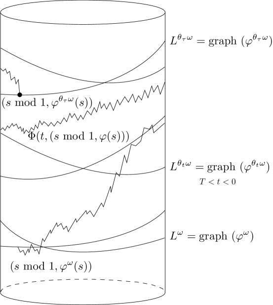
use a random quasi-periodic winding system on S1Γ—YΟ‰superscript𝑆1superscriptπ‘Œπœ”S^{1}\times Y^{\omega} to characterize the invariant set XΟ‰superscriptπ‘‹πœ”X^{\omega} further and to study the existence of random periodic curves on the cylinder. We will prove under the following three conditions, the invariant set XΟ‰superscriptπ‘‹πœ”X^{\omega} consists of a finite number of periodic curves. The Lyapunov exponent and the pullback are key techniques in our approach. So it is essential to assume the random dynamical systems are C1superscript𝐢1C^{1} perfect cocycles. It is known from the works of many mathematicians that cocycles can be generated from some random differential equations and stochastic differential equations (c.f. Arnold arnold ).

Condition (i) Assume that there exists a random compact subset Y of $R^{d}$ and $t_{1}>0$ such that for any $s\in S^{1}$ and $y=(x_{1},x_{2},\cdots,x_{d})\in Y^{\omega}$ (denote $z_{0}=(s,x_{1},\cdots,x_{d}))$, $\gamma_{z_{0}}^{\omega}(t_{1})=(s^{\prime},x_{1}^{\prime},\cdots,x_{d}^{\prime})$ with

$\displaystyle s^{\prime}=s+1,$ (9)

and

$\displaystyle y^{\prime}=(x_{1}^{\prime},x_{2}^{\prime},\cdots,x_{d}^{\prime})\in Y^{\theta_{t_{1}}\omega}.$ (10)

We assume there is an invariant compact set $X^{\omega}\subset S^{1}\times Y^{\omega}$, that is to say $X^{\omega}$ satisfies

$\displaystyle\gamma^{\omega}(t)X^{\omega}=X^{\theta_{t}\omega},$ (11)

for all $t\in R$ and the projection of $X^{\omega}$ to the subspace $S^{1}$ is $S^{1}$, there exist a constant $b^{*}>0$ such that $|X^{\omega}|<b^{*}$ where $|X^{\omega}|$ denotes the diameter of $X^{\omega}$ in the y-direction.

Note that $t_{1}$ is the time that a particle on $S^{1}$ rotate a full circle, no matter where it starts, (10) is just an invariant condition about the random compact subset $Y^{\omega}\subset R^{d}$.

In the following, we denote $\hat{\theta}\omega=\theta_{t_{1}}\omega$. Under the above assumption, a random winding system can be defined from the continuous time $C^{1}$ random dynamical system $\gamma$ by letting

h​(s)=sβ€²β„Žπ‘ superscript𝑠′h(s)=s^{\prime}

and

gω​(s,y)=yβ€².superscriptπ‘”πœ”π‘ π‘¦superscript𝑦′g^{\omega}(s,y)=y^{\prime}.

Consider the following discrete time random winding system

$\displaystyle\left\{\begin{array}[]{l}s_{n+1}=h(s_{n}){{\rm\ mod\ }}1,s_{n}\in S^{1}\cr y_{n+1}=g^{\omega}(s_{n},y_{n}),\hskip 12.80365pty_{n}\in R^{d},\end{array}\right.$ (14)

where $S^{1}$ is the unit circle, $g:\Omega\times S^{1}\times R^{d}\to R^{d}$ is ${\cal F}\otimes{\cal B}(S^{1})\otimes{\cal B}(R^{d})$, ${\cal B}(R^{d})$ measurable and $g^{\omega}:S^{1}\times R^{d}\to R^{d}$ is jointly continuous for each $\omega$ and gω​(s,β‹…):Rdβ†’Rd:superscriptπ‘”πœ”π‘ β‹…β†’superscript𝑅𝑑superscript𝑅𝑑g^{\omega}(s,\cdot):R^{d}\to R^{d} is differentiable for each (Ο‰,s)βˆˆΞ©Γ—S1πœ”π‘ Ξ©superscript𝑆1(\omega,s)\in\Omega\times S^{1}. To be convenient, denote

Hω​(s,y)=(h​(s)​mod​ 1,gω​(s,y)),superscriptπ»πœ”π‘ π‘¦β„Žπ‘ mod1superscriptπ‘”πœ”π‘ π‘¦\displaystyle H^{\omega}(s,y)=(h(s){{\rm\ mod\ }}1,g^{\omega}(s,y)), (15)

for the skew product map on $S^{1}\times R^{d}$. We shall also define $g^{(n)}$ iteratively by H(n),ω​(s,y)=(h(n)​(s)​mod​ 1,g(n),ω​(s,y))superscriptπ»π‘›πœ”π‘ π‘¦superscriptβ„Žπ‘›π‘ mod1superscriptπ‘”π‘›πœ”π‘ π‘¦H^{(n),\omega}(s,y)=(h^{(n)}(s){{\rm\ mod\ }}1,g^{(n),\omega}(s,y)). It is easy to know that $\hat{\theta}:\{\cdots,-3,-2,-1,0,1,2,3,\cdots\}\times\Omega\to\Omega$ is a $P$-preserving map such that for all $m,n\in\{\cdots,-3,-2,-1,0,1,2,3,\cdots\}$

H(m+n),ω​(s,y)=H(m),ΞΈ^n​ω​(H(n),ω​(s,y)),superscriptπ»π‘šπ‘›πœ”π‘ π‘¦superscriptπ»π‘šsuperscript^πœƒπ‘›πœ”superscriptπ»π‘›πœ”π‘ π‘¦\displaystyle H^{(m+n),\omega}(s,y)=H^{(m),\hat{\theta}^{n}\omega}(H^{(n),\omega}(s,y)), (16)

for all $(s,y)\in S^{1}\times R^{d}$ almost surely.

Let $\pi:R\times R^{d}\rightarrow S^{1}\times R^{d}$ be the natural covering $\pi(a,y)=(a\hskip 5.69046ptmod\hskip 2.84544pt1,y)$ and $\varphi^{\omega}$ a periodic continuous function. If $\pi({\rm graph}\hskip 5.69046pt\varphi)$ is invariant under $(H,\hat{\theta})$, that is to say that $H^{\hat{\theta}^{-1}\omega}\pi({\rm graph}\hskip 5.69046pt\varphi^{\hat{\theta}^{-1}\omega})=\pi({\rm graph}\hskip 5.69046pt\varphi^{\omega})$ a.s., it is said that $\varphi$ is an invariant curve for the skew product (15).

To analyse the structure of $X^{\omega}$, we pose the following conditions.

Condition (ii) Assume that there exists $\delta_{1}>0$ and $L_{1}>0$ such that for any $(s,y)\in X^{\omega}$, there exists a Lipschitz continuous function $f:S^{1}\to R^{d}$ with Lipschitz constant $L_{1}$ and $f(s)=y$ such that $(s^{*},f(s^{*}))\in X^{\omega}$ when $s^{*}\in[s-\delta_{1},s+\delta_{1}]$.

Define the $(\delta,\varepsilon)$ neighbourhood of $(s,y)\in X^{\omega}$ and $X^{\omega}$ as

B​(s,y,Ξ΄,Ξ΅)={(sβ€²,yβ€²):sβ€²βˆˆ[sβˆ’Ξ΄,s+Ξ΄],β€–yβ€²βˆ’f​(sβ€²)‖≀Ρ},π΅π‘ π‘¦π›Ώπœ€conditional-setsuperscript𝑠′superscript𝑦′formulae-sequencesuperscript𝑠′𝑠𝛿𝑠𝛿normsuperscript𝑦′𝑓superscriptπ‘ β€²πœ€\displaystyle B(s,y,\delta,\varepsilon)=\{(s^{\prime},y^{\prime}):s^{\prime}\in[s-\delta,s+\delta],||y^{\prime}-f(s^{\prime})||\leq\varepsilon\},

and, for any $s\in S^{1}$,

Bs​(Ξ΄,Ξ΅)=⋃(s,y)∈XΟ‰B​(s,y,Ξ΄,Ξ΅),subscriptπ΅π‘ π›Ώπœ€subscript𝑠𝑦superscriptπ‘‹πœ”π΅π‘ π‘¦π›Ώπœ€{B}_{s}(\delta,\varepsilon)=\bigcup_{(s,y)\in X^{\omega}}B(s,y,\delta,\varepsilon),

and

B​(XΟ‰,Ξ΅)=⋃s∈S1Bs​(Ξ΄,Ξ΅),𝐡superscriptπ‘‹πœ”πœ€subscript𝑠superscript𝑆1subscriptπ΅π‘ π›Ώπœ€{B}(X^{\omega},\varepsilon)=\bigcup_{s\in S^{1}}B_{s}(\delta,\varepsilon),

respectively. In fact, Bs​(Ξ΄,Ξ΅)subscriptπ΅π‘ π›Ώπœ€{B}_{s}(\delta,\varepsilon) is the $\varepsilon$-neighbourhood of XΟ‰βˆ©([sβˆ’Ξ΄,s+Ξ΄]Γ—YΟ‰)superscriptπ‘‹πœ”π‘ π›Ώπ‘ π›Ώsuperscriptπ‘Œπœ”X^{\omega}\cap([s-\delta,s+\delta]\times Y^{\omega}) in the $y$-direction and ${B}(X^{\omega},\varepsilon)$ is the $\varepsilon$-neighbourhood of $X^{\omega}$ in the $y$-direction. Note that ⋃s∈S1Bs​(Ξ΄,Ξ΅)subscript𝑠superscript𝑆1subscriptπ΅π‘ π›Ώπœ€\bigcup_{s\in S^{1}}B_{s}(\delta,\varepsilon) does not depend on $\delta$.

Condition (iii) Assume there exists an $\lambda<1$, $\varepsilon_{1}>0$ and an $n_{0}\in\hbox{\lou N}$ such that for almost all $\omega\in\Omega$,

β€–Dy​g(n0),ω​(s,y)‖≀λ​for​all​(s,y)∈B​(XΟ‰,Ξ΅1),normsubscript𝐷𝑦superscript𝑔subscript𝑛0πœ”π‘ π‘¦πœ†forall𝑠𝑦𝐡superscriptπ‘‹πœ”subscriptπœ€1\displaystyle||D_{y}g^{(n_{0}),\omega}(s,y)||\leq\lambda{\rm\ for\ all\ }(s,y)\in B(X^{\omega},\varepsilon_{1}), (17)

and

c=ess​supΟ‰sup(s,y)∈B​(XΟ‰,Ξ΅1)β€–βˆ‚g(n0),Ο‰βˆ‚s​(s,y)β€–<+∞,𝑐esssubscriptsupremumπœ”subscriptsupremum𝑠𝑦𝐡superscriptπ‘‹πœ”subscriptπœ€1normsuperscript𝑔subscript𝑛0πœ”π‘ π‘ π‘¦\displaystyle c={\rm ess}\sup_{\hskip-15.0pt\omega}\sup_{(s,y)\in{B}(X^{\omega},\varepsilon_{1})}||\frac{\partial g^{(n_{0}),\omega}}{\partial s}(s,y)||<+\infty, (18)

This assumption can be understood as a condition on the amplitude of Lyapunov exponent of the random map. It is not difficult to prove that for all $m\in\hbox{\lou N}$

$\displaystyle H^{mn_{0},{\omega}}(B(X^{\omega},\varepsilon_{1}))\subset{B}(X^{\hat{\theta}^{mn_{0}}\omega},\varepsilon_{1}).$ (19)

That is to say that there exists a forward random invariant compact set $B(X^{\omega},\varepsilon_{1})$. By the chain rule, for all $(s,y)\in B(X^{\omega},\varepsilon_{1})$ and $m\in\hbox{\lou N}$,

β€–Dy​gs(m​n0),ω​(y)‖≀λm.normsubscript𝐷𝑦superscriptsubscriptπ‘”π‘ π‘šsubscript𝑛0πœ”π‘¦superscriptπœ†π‘š\displaystyle||D_{y}g_{s}^{(mn_{0}),\omega}(y)||\leq\lambda^{m}. (20)

Moreover, it is easy to see that for any $(s,y)\in X^{\omega}$,

Hm​n0,ω​(B​(s,y,Ξ΄1,Ξ΅1))βŠ‚B​(Hm​n0,ω​(s,y),Ξ΄1,Ξ΅1),superscriptπ»π‘šsubscript𝑛0πœ”π΅π‘ π‘¦subscript𝛿1subscriptπœ€1𝐡superscriptπ»π‘šsubscript𝑛0πœ”π‘ π‘¦subscript𝛿1subscriptπœ€1\displaystyle H^{mn_{0},\omega}(B(s,y,\delta_{1},\varepsilon_{1}))\subset{B}(H^{mn_{0},\omega}(s,y),\delta_{1},\varepsilon_{1}), (21)

and for any $(s^{\prime},y_{1}),(s^{\prime},y_{2})\in B(s,y,\delta_{1},\varepsilon_{1})$,

$\displaystyle H^{mn_{0},\omega}(s^{\prime},y_{1})$ $\displaystyle=$ (sβ€²+m​n0​mod​ 1,gsβ€²(m​n0),ω​(y1))∈B​(Hm​n0,ω​(s,y),Ξ΄1,Ξ΅1),superscriptπ‘ β€²π‘šsubscript𝑛0mod1superscriptsubscript𝑔superscriptπ‘ β€²π‘šsubscript𝑛0πœ”subscript𝑦1𝐡superscriptπ»π‘šsubscript𝑛0πœ”π‘ π‘¦subscript𝛿1subscriptπœ€1\displaystyle(s^{\prime}+mn_{0}\ {\rm mod}\ 1,g_{s^{\prime}}^{(mn_{0}),\omega}(y_{1}))\in B(H^{mn_{0},\omega}(s,y),\delta_{1},\varepsilon_{1}),
$\displaystyle H^{mn_{0},\omega}(s^{\prime},y_{2})$ $\displaystyle=$ (sβ€²+m​n0​mod​ 1,gsβ€²(m​n0),ω​(y2))∈B​(Hm​n0,ω​(s,y),Ξ΄1,Ξ΅1)superscriptπ‘ β€²π‘šsubscript𝑛0mod1superscriptsubscript𝑔superscriptπ‘ β€²π‘šsubscript𝑛0πœ”subscript𝑦2𝐡superscriptπ»π‘šsubscript𝑛0πœ”π‘ π‘¦subscript𝛿1subscriptπœ€1\displaystyle(s^{\prime}+mn_{0}\ {\rm mod}\ 1,g_{s^{\prime}}^{(mn_{0}),\omega}(y_{2}))\in B(H^{mn_{0},\omega}(s,y),\delta_{1},\varepsilon_{1})

and

β€–gsβ€²(m​n0),ω​(y1)βˆ’gsβ€²(m​n0),ω​(y2)‖≀λm​‖y1βˆ’y2β€–.normsuperscriptsubscript𝑔superscriptπ‘ β€²π‘šsubscript𝑛0πœ”subscript𝑦1superscriptsubscript𝑔superscriptπ‘ β€²π‘šsubscript𝑛0πœ”subscript𝑦2superscriptπœ†π‘šnormsubscript𝑦1subscript𝑦2\displaystyle||g_{s^{\prime}}^{(mn_{0}),\omega}(y_{1})-g_{s^{\prime}}^{(mn_{0}),\omega}(y_{2})||\leq\lambda^{m}||y_{1}-y_{2}||. (22)

From this, it is easy to see that $X^{\omega}$ actually is a random attractor. The main aim of this section is to prove the following theorem.

Theorem 3.2

Under Conditions (i), (ii), (iii), the cocycle $\gamma$ has $r^{\omega}$ random periodic solutions of period $t_{i}^{*\omega}$ with random periodic curve $L_{i}^{\omega}$ of winding number $\tau_{i}^{\omega}$, $i=1,2,\cdots,r$. Moreover, for any $t\in R$, $r^{\theta_{-t}\omega}=r^{\omega}$, and $t_{i}^{*\theta_{-t}\omega}=t_{i}^{*\omega}$, $\tau_{i}^{\theta_{-t}\omega}=\tau_{i}^{\omega}$ for each $i=1,2,\cdots,r^{\omega}$.

We need a series of preparations to prove this theorem. First, for any $s\in S^{1}$, let’s define

XsΟ‰=XΟ‰βˆ©({s}Γ—YΟ‰).superscriptsubscriptπ‘‹π‘ πœ”superscriptπ‘‹πœ”π‘ superscriptπ‘Œπœ”X_{s}^{\omega}=X^{\omega}\cap(\{s\}\times Y^{\omega}).

Let GsΟ‰superscriptsubscriptπΊπ‘ πœ”G_{s}^{\omega} be a connected component of XsΟ‰superscriptsubscriptπ‘‹π‘ πœ”X_{s}^{\omega}. For any $y_{1},y_{2}\in R^{d}$ and (s,y1),(s,y2)∈Gsω𝑠subscript𝑦1𝑠subscript𝑦2superscriptsubscriptπΊπ‘ πœ”(s,y_{1}),(s,y_{2})\in G_{s}^{\omega}, there exist $y_{1}^{\prime},y_{2}^{\prime}\in R^{d}$ with $(s^{\prime},y_{1}^{\prime}),(s^{\prime},y_{2}^{\prime})\in X^{\hat{\theta}^{-mn_{0}}\omega}$ such that

sβ€²+m​n0​mod​ 1=s,gsβ€²m​n0,ΞΈ^βˆ’m​n0​ω​(y1β€²)=y1,gsβ€²m​n0,ΞΈ^βˆ’m​n0​ω​(y2β€²)=y2,formulae-sequencesuperscriptπ‘ β€²π‘šsubscript𝑛0mod1𝑠formulae-sequencesuperscriptsubscript𝑔superscriptπ‘ β€²π‘šsubscript𝑛0superscript^πœƒπ‘šsubscript𝑛0πœ”superscriptsubscript𝑦1β€²subscript𝑦1superscriptsubscript𝑔superscriptπ‘ β€²π‘šsubscript𝑛0superscript^πœƒπ‘šsubscript𝑛0πœ”superscriptsubscript𝑦2β€²subscript𝑦2\displaystyle s^{\prime}+mn_{0}\ {\rm mod}\ 1=s,\ g_{s^{\prime}}^{mn_{0},\hat{\theta}^{-mn_{0}}\omega}(y_{1}^{\prime})=y_{1},\ g_{s^{\prime}}^{mn_{0},\hat{\theta}^{-mn_{0}}\omega}(y_{2}^{\prime})=y_{2},

and

$\displaystyle||y_{1}-y_{2}||\leq\lambda^{m}||y_{1}^{\prime}-y_{2}^{\prime}||.$ (23)

Let |GsΟ‰|superscriptsubscriptπΊπ‘ πœ”|G_{s}^{\omega}| be the largest radius of the set GsΟ‰superscriptsubscriptπΊπ‘ πœ”G_{s}^{\omega}. Define

|GΟ‰|=sups∈S1|GsΟ‰|.superscriptπΊπœ”subscriptsupremum𝑠superscript𝑆1superscriptsubscriptπΊπ‘ πœ”|G^{\omega}|=\sup_{s\in S^{1}}|G_{s}^{\omega}|.

Set for $l>0$

$$\Omega_{0}^{l}=\{\omega:|G^{\omega}|\geq l\}.$$

Then we have

Lemma 3.3

For any $l>0$,

$\displaystyle P(\Omega_{0}^{l})=0.$ (24)

Proof. Assume the claim of the lemma is not true, i.e. there exists $\alpha_{l}>0$ such that $P(\Omega_{0}^{l})=\alpha_{l}$. Also define

$$\Omega_{m}^{l}=\{\omega:|G^{\omega}|\geq{l\over\lambda^{m}}\}.$$

Then from the invariance of $X^{\omega}$, the Conditions (ii) and (iii) and (23), we know that

$$\hat{\theta}^{m}\left((\Omega_{m}^{l})^{c}\right)\subset(\Omega_{0}^{l})^{c}.$$

So

$$\hat{\theta}^{m}\left(\Omega_{m}^{l}\right)\supset\Omega_{0}^{l}.$$

Now as $\hat{\theta}$ is measure preserving we know that for any $m\geq 0$,

$\displaystyle P\left(\Omega_{m}^{l}\right)=P\left(\hat{\theta}^{m}\Omega_{m}^{l}\right)\geq P\left(\Omega_{0}^{l}\right)=\alpha_{l}>0.$ (25)

Note that $\Omega_{m}^{l}\downarrow\emptyset$. So by the continuity of probability measure with respect to decreasing sequence of sets, we have as $m\to+\infty$

$\displaystyle P\left(\Omega_{m}^{l}\right)\to 0.$ (26)

Clearly, (25) and (26) contradict each other. The lemma is proved. β– β– \blacksquare

In the following, we will use the pullback of random maps (arnold ), the PoincarΓ© map, and the Lyapunov exponent to prove that $X^{\omega}$ is a union of finite number of Lipschitz periodic curves. That is to say that there exists $r^{\omega}$ continuous periodic functions $\varphi_{1}^{\omega}$, $\varphi_{2}^{\omega},\cdots,\varphi_{r^{\omega}}^{\omega}$ on $R^{1}$ with periods $\tau_{1}^{\omega},\tau_{2}^{\omega},\cdots,\tau_{r^{\omega}}^{\omega}\in\hbox{\lou N}$ respectively such that

$\displaystyle X^{\omega}=L_{1}^{\omega}\cup L_{2}^{\omega}\cup\cdots\cup L_{r^{\omega}}^{\omega},$ (27)

where

LiΟ‰=graph​(Ο†iΟ‰)={(s​mod​ 1,Ο†iω​(s)):s∈[0,Ο„iΟ‰)},i=1,2,β‹―,rΟ‰,formulae-sequencesuperscriptsubscriptπΏπ‘–πœ”graphsuperscriptsubscriptπœ‘π‘–πœ”conditional-set𝑠mod1subscriptsuperscriptπœ‘πœ”π‘–π‘ π‘ 0superscriptsubscriptπœπ‘–πœ”π‘–12β‹―superscriptπ‘Ÿπœ”\displaystyle L_{i}^{\omega}={\rm graph}(\varphi_{i}^{\omega})=\{(s{\rm\ mod\ }1,\varphi^{\omega}_{i}(s)):s\in[0,\tau_{i}^{\omega})\},\ i=1,2,\cdots,r^{\omega}, (28)

are invariant under $(H,\hat{\theta})$. Some estimates in the proof of the following lemmas (Lemma 3.4-Proposition 3.9) are the extension of the results in stark to the stochastic case. This is not trivial and the pullback technique has to be used to make the estimates work. Moreover, it is essential to prove that

$\displaystyle\tau_{i}^{\theta_{-t}\omega}=\tau_{i}^{\omega}\ {\rm and}\ r^{\theta_{-t}\omega}=r^{\omega}$ (29)

for all $t\in R$. The fact that the periodic curves are not the trajectories of the random dynamical system, and the fact that the periodic curves are different corresponding to different $\omega$, make it difficult to follow the trajectories of the random dynamical systems. The essential difficulty in the stochastic case arises from the fact that although $X^{\omega}$ is a random invariant set satisfying (11), but in general, $X^{\omega}$ and $\gamma^{\omega}(t)X^{\omega}$ are different sets. The set $X^{\omega}$ is not invariant in the sense as in the deterministic case. This is fundamentally different from the deterministic case. As a consequence, the neighbourhood of $X^{\omega}$ is only forward invariant in the sense of (19). The assumption (20) makes the $(\delta_{1},\varepsilon_{1})$-neighbourhood of $X^{\omega}$ under the map $H^{mn_{0},\omega}$ contracting in the $y$-direction to the $(\delta_{1},\varepsilon_{1})$-neighbourhood of $X^{\hat{\theta}^{mn_{0}}\omega}$, rather than the $(\delta_{1},\varepsilon_{1})$-neighbourhood of $X^{\omega}$ as in the deterministic case. Locally, (21) says the map $H^{mn_{0},\omega}$ maps the $(\delta_{1},\varepsilon_{1})$-neighbourhood of $(s,y)\in X^{\omega}$ to the $(\delta_{1},\varepsilon_{1})$-neighbourhood of Hm​n0,ω​(s,y)∈XΞΈ^m​n0​ωsuperscriptπ»π‘šsubscript𝑛0πœ”π‘ π‘¦superscript𝑋superscript^πœƒπ‘šsubscript𝑛0πœ”H^{mn_{0},\omega}(s,y)\in X^{\hat{\theta}^{mn_{0}}\omega}. Here, unlike the deterministic case, Hm​n0,ω​(s,y)superscriptπ»π‘šsubscript𝑛0πœ”π‘ π‘¦H^{mn_{0},\omega}(s,y) is not on the same $X^{\cdot}$ as $(s,y)$ is.

To prove the above claim, for $(s,y)\in B(X^{\omega},\varepsilon_{1})\subset S^{1}\times Y^{\omega},$ denote

$\displaystyle{h_{1}(s)}$ $\displaystyle=$ $\displaystyle{h^{(n_{0})}(s)},$
g1ω​(s,y)superscriptsubscript𝑔1πœ”π‘ π‘¦\displaystyle g_{1}^{\omega}(s,y) $\displaystyle=$ g(n0),ω​(s,y)=gΞΈ^n0βˆ’1​ω​(h(n0βˆ’1)​(s),g(n0βˆ’1),ω​(s,y)),superscript𝑔subscript𝑛0πœ”π‘ π‘¦superscript𝑔superscript^πœƒsubscript𝑛01πœ”superscriptβ„Žsubscript𝑛01𝑠superscript𝑔subscript𝑛01πœ”π‘ π‘¦\displaystyle{g^{(n_{0}),\omega}}(s,y)=g^{\hat{\theta}^{n_{0}-1}\omega}(h^{(n_{0}-1)}(s),g^{(n_{0}-1),\omega}(s,y)),
H1ω​(s,y)superscriptsubscript𝐻1πœ”π‘ π‘¦\displaystyle H_{1}^{\omega}(s,y) $\displaystyle=$ (h1​(s),g1ω​(s,y)).subscriptβ„Ž1𝑠superscriptsubscript𝑔1πœ”π‘ π‘¦\displaystyle(h_{1}(s),g_{1}^{\omega}(s,y)).

For any $(s^{*},y^{*})\ \in\ S_{1}\times Y^{\hat{\theta}^{-mn_{0}}\omega}$, define

$$\xi_{m}^{\hat{\theta}^{-mn_{0}}\omega}:[h_{1}^{m}(s^{*})-\delta_{1},h_{1}^{m}(s^{*})+\delta_{1}]\to Y^{\omega}$$

by an induction:

ΞΎ0ΞΈ^βˆ’m​n0​ω​(s)superscriptsubscriptπœ‰0superscript^πœƒπ‘šsubscript𝑛0πœ”π‘ \displaystyle\xi_{0}^{\hat{\theta}^{-mn_{0}}\omega}(s) $\displaystyle=$ $\displaystyle f(s)\in Y^{\hat{\theta}^{-mn_{0}}\omega},\forall s\in[s^{*}-\delta_{1},s^{*}+\delta_{1}],$
ΞΎ1ΞΈ^βˆ’m​n0​ω​(s)superscriptsubscriptπœ‰1superscript^πœƒπ‘šsubscript𝑛0πœ”π‘ \displaystyle\xi_{1}^{\hat{\theta}^{-mn_{0}}\omega}(s) $\displaystyle=$ $\displaystyle g_{1}^{\hat{\theta}^{-mn_{0}}\omega}(h_{1}^{-1}(s),\ \xi_{0}^{\hat{\theta}^{-mn_{0}}\omega}(h_{1}^{-1}(s)))\in Y^{\hat{\theta}^{-(m-1)n_{0}}\omega},$
$\displaystyle\qquad\qquad\forall s\in[h_{1}(s^{*})-\delta_{1},\ h_{1}(s^{*})+\delta_{1}],$

and

ΞΎmΞΈ^βˆ’m​n0​ω​(s)superscriptsubscriptπœ‰π‘šsuperscript^πœƒπ‘šsubscript𝑛0πœ”π‘ \displaystyle\xi_{m}^{\hat{\theta}^{-mn_{0}}\omega}(s) $\displaystyle=$ $\displaystyle g_{1}^{\hat{\theta}^{-n_{0}}\omega}(h_{1}^{-1}(s),\ \xi_{m-1}^{\hat{\theta}^{-mn_{0}}\omega}(h_{1}^{-1}(s)))\in Y^{\omega},$
$\displaystyle\quad\forall s\in[h_{1}^{m}(s^{*})-\delta_{1},\ h_{1}^{m}(s^{*})+\delta_{1}].$

Denote

$$\delta_{2}=min\{\frac{\delta_{1}}{2},\frac{\varepsilon_{1}}{4L_{1}}\}\ \ and\ \ L=\frac{c}{1-\lambda}.$$
Lemma 3.4

Under Conditions (i), (ii), (iii), the function $\xi_{i}^{\hat{\theta}^{-mn_{0}}\omega}$ is Lipschitz continuous with a Lipschitz constant $L$ for all $m\in\hbox{\lou N}$ and $i=1,2,\cdots,m$, that is, for any $m\in\hbox{\lou N}$ and $i=1,2,\cdots,m$,

(s,ΞΎiΞΈ^βˆ’m​n0​ω​(s)),(sβ€²,ΞΎiΞΈ^βˆ’m​n0​ω​(sβ€²))∈B​(XΞΈ^βˆ’(mβˆ’i)​n0​ω,Ξ΅1),𝑠superscriptsubscriptπœ‰π‘–superscript^πœƒπ‘šsubscript𝑛0πœ”π‘ superscript𝑠′superscriptsubscriptπœ‰π‘–superscript^πœƒπ‘šsubscript𝑛0πœ”superscript𝑠′𝐡superscript𝑋superscript^πœƒπ‘šπ‘–subscript𝑛0πœ”subscriptπœ€1\displaystyle(s,\xi_{i}^{\hat{\theta}^{-mn_{0}}\omega}(s)),(s^{\prime},\xi_{i}^{\hat{\theta}^{-mn_{0}}\omega}(s^{\prime}))\in B(X^{\hat{\theta}^{-(m-i)n_{0}}\omega},\varepsilon_{1}),

and

β€–ΞΎiΞΈ^βˆ’m​n0​ω​(s)βˆ’ΞΎiΞΈ^βˆ’m​n0​ω​(sβ€²)‖≀L​|sβˆ’sβ€²|,normsuperscriptsubscriptπœ‰π‘–superscript^πœƒπ‘šsubscript𝑛0πœ”π‘ superscriptsubscriptπœ‰π‘–superscript^πœƒπ‘šsubscript𝑛0πœ”superscript𝑠′𝐿𝑠superscript𝑠′\displaystyle\|\xi_{i}^{\hat{\theta}^{-mn_{0}}\omega}(s)-\xi_{i}^{\hat{\theta}^{-mn_{0}}\omega}(s^{\prime})\|\leq L|s-s^{\prime}|,

for any $s,\ s^{\prime}\in[h_{1}^{i}(s^{*})-\delta_{2},\ h_{1}^{i}(s^{*})+\delta_{2}].$

Proof  We prove this lemma by the induction on $i=1,2,\cdots,m$ for an arbitrary $m$. When $i=1$ and $s,\ s^{\prime}\in[h_{1}(s^{*})-\delta_{2},\ h_{1}(s^{*})+\delta_{2}]$, by (18), we have

β€–ΞΎ1ΞΈ^βˆ’m​n0​ω​(s)βˆ’ΞΎ1ΞΈ^βˆ’m​n0​ω​(sβ€²)β€–normsuperscriptsubscriptπœ‰1superscript^πœƒπ‘šsubscript𝑛0πœ”π‘ superscriptsubscriptπœ‰1superscript^πœƒπ‘šsubscript𝑛0πœ”superscript𝑠′\displaystyle\|\xi_{1}^{\hat{\theta}^{-mn_{0}}\omega}(s)-\xi_{1}^{\hat{\theta}^{-mn_{0}}\omega}(s^{\prime})\|
$\displaystyle=$ $\displaystyle|g_{1}^{\hat{\theta}^{-mn_{0}}\omega}\ (h_{1}^{-1}(s),\ f(s))-g_{1}^{\hat{\theta}^{-mn_{0}}\omega}(h_{1}^{-1}(s^{\prime}),\ f(s))\|$
$\displaystyle\leq$ $\displaystyle c|h_{1}^{-1}(s)-h_{1}^{-1}(s^{\prime})|$
$\displaystyle<$ $\displaystyle L|s-s^{\prime}|,$

and by (19), we have (s,ΞΎ1ΞΈ^βˆ’m​n0​ω​(s)),(sβ€²,ΞΎ1ΞΈ^βˆ’m​n0​ω​(sβ€²))∈B​(XΞΈ^βˆ’(mβˆ’1)​n0​ω,Ξ΅1)𝑠superscriptsubscriptπœ‰1superscript^πœƒπ‘šsubscript𝑛0πœ”π‘ superscript𝑠′superscriptsubscriptπœ‰1superscript^πœƒπ‘šsubscript𝑛0πœ”superscript𝑠′𝐡superscript𝑋superscript^πœƒπ‘š1subscript𝑛0πœ”subscriptπœ€1(s,\xi_{1}^{\hat{\theta}^{-mn_{0}}\omega}(s)),(s^{\prime},\xi_{1}^{\hat{\theta}^{-mn_{0}}\omega}(s^{\prime}))\in B(X^{\hat{\theta}^{-(m-1)n_{0}}\omega},\varepsilon_{1}). Now suppose the required result holds for $i-1\in\{1,2,\cdots,m-1\}$, then for any $s,\ s^{\prime}\in[h_{1}^{i}(s^{*})-\delta_{2},\ h_{1}^{i}(s^{*})+\delta_{2}]$

β€–ΞΎiΞΈ^βˆ’m​n0​ω​(s)βˆ’ΞΎiΞΈ^βˆ’m​n0​ω​(sβ€²)β€–normsuperscriptsubscriptπœ‰π‘–superscript^πœƒπ‘šsubscript𝑛0πœ”π‘ superscriptsubscriptπœ‰π‘–superscript^πœƒπ‘šsubscript𝑛0πœ”superscript𝑠′\displaystyle\|\xi_{i}^{\hat{\theta}^{-mn_{0}}\omega}(s)-\xi_{i}^{\hat{\theta}^{-mn_{0}}\omega}(s^{\prime})\|
$\displaystyle=$ $\displaystyle\|g_{1}^{\hat{\theta}^{-n_{0}}\omega}\ (h_{1}^{-1}(s),\ \xi_{i-1}^{\hat{\theta}^{-mn_{0}}\omega}(h_{1}^{-1}(s)))-g_{1}^{\hat{\theta}^{-n_{0}}\omega}\ (h_{1}^{-1}(s^{\prime}),\ \xi_{i-1}^{\hat{\theta}^{-mn_{0}}\omega}(h_{1}^{-1}(s^{\prime})))||$
$\displaystyle\leq$ $\displaystyle|g_{1}^{\hat{\theta}^{-n_{0}}\omega}(h_{1}^{-1}(s),\ \xi_{i-1}^{\hat{\theta}^{-mn_{0}}\omega}(h_{1}^{-1}(s)))-g_{1}^{\hat{\theta}^{-n_{0}}\omega}(h_{1}^{-1}(s^{\prime}),\ \xi_{i-1}^{\hat{\theta}^{-mn_{0}}\omega}(h_{1}^{-1}(s)))\|$
$\displaystyle+\|g_{1}^{\hat{\theta}^{-n_{0}}\omega}(h_{1}^{-1}(s^{\prime}),\ \xi_{i-1}^{\hat{\theta}^{-mn_{0}}\omega}(h_{1}^{-1}(s)))-g_{1}^{\hat{\theta}^{-n_{0}}\omega}(h_{1}^{-1}(s^{\prime}),\ \xi_{i-1}^{\hat{\theta}^{-mn_{0}}\omega}(h_{1}^{-1}(s^{\prime})))\|$
$\displaystyle\leq$ c​|h1βˆ’1​(s)βˆ’h1βˆ’1​(sβ€²)|+λ​‖ξiβˆ’1ΞΈ^βˆ’m​n0​ω​(h1βˆ’1​(s))βˆ’ΞΎiβˆ’1ΞΈ^βˆ’m​n0​ω​(h1βˆ’1​(sβ€²))‖𝑐superscriptsubscriptβ„Ž11𝑠superscriptsubscriptβ„Ž11superscriptπ‘ β€²πœ†normsuperscriptsubscriptπœ‰π‘–1superscript^πœƒπ‘šsubscript𝑛0πœ”superscriptsubscriptβ„Ž11𝑠superscriptsubscriptπœ‰π‘–1superscript^πœƒπ‘šsubscript𝑛0πœ”superscriptsubscriptβ„Ž11superscript𝑠′\displaystyle c|h_{1}^{-1}(s)-h_{1}^{-1}(s^{\prime})|+\lambda\|\xi_{i-1}^{\hat{\theta}^{-mn_{0}}\omega}(h_{1}^{-1}(s))-\xi_{i-1}^{\hat{\theta}^{-mn_{0}}\omega}(h_{1}^{-1}(s^{\prime}))\|
$\displaystyle\leq$ (c+λ​L)​|sβˆ’sβ€²|π‘πœ†πΏπ‘ superscript𝑠′\displaystyle(c+\lambda L)|s-s^{\prime}|
$\displaystyle\leq$ $\displaystyle L|s^{\prime}-s|,$

and the claim (s,ΞΎiΞΈ^βˆ’m​n0​ω​(s)),(sβ€²,ΞΎiΞΈ^βˆ’m​n0​ω​(sβ€²))∈B​(XΞΈ^βˆ’(mβˆ’i)​n0​ω,Ξ΅1)𝑠superscriptsubscriptπœ‰π‘–superscript^πœƒπ‘šsubscript𝑛0πœ”π‘ superscript𝑠′superscriptsubscriptπœ‰π‘–superscript^πœƒπ‘šsubscript𝑛0πœ”superscript𝑠′𝐡superscript𝑋superscript^πœƒπ‘šπ‘–subscript𝑛0πœ”subscriptπœ€1(s,\xi_{i}^{\hat{\theta}^{-mn_{0}}\omega}(s)),(s^{\prime},\xi_{i}^{\hat{\theta}^{-mn_{0}}\omega}(s^{\prime}))\in B(X^{\hat{\theta}^{-(m-i)n_{0}}\omega},\varepsilon_{1}) follows from (19). The lemma is proved. β– β– \blacksquare

For any (s,y)∈Xsω𝑠𝑦superscriptsubscriptπ‘‹π‘ πœ”(s,y)\in X_{s}^{\omega}, let $N(s,y,\delta_{2},\varepsilon_{1})$ be the interior of Bω​(s,y,Ξ΄2,Ξ΅1)superscriptπ΅πœ”π‘ π‘¦subscript𝛿2subscriptπœ€1B^{\omega}(s,y,\delta_{2},\varepsilon_{1}). Then for any $s^{*}\in S^{1}$, {N​(sβˆ—,y,Ξ΄2,Ξ΅1)|(sβˆ—,y)∈Xsβˆ—Ο‰}conditional-set𝑁superscript𝑠𝑦subscript𝛿2subscriptπœ€1superscript𝑠𝑦superscriptsubscript𝑋superscriptπ‘ πœ”\{N(s^{*},y,\delta_{2},\varepsilon_{1})\big{|}(s^{*},y)\in X_{s^{*}}^{\omega}\} is an open covering of Xsβˆ—Ο‰superscriptsubscript𝑋superscriptπ‘ πœ”X_{s^{*}}^{\omega}. By compactness of Xsβˆ—Ο‰superscriptsubscript𝑋superscriptπ‘ πœ”X_{s^{*}}^{\omega}, a finite subcover, $N(s^{*},y^{(1)}_{\omega},\delta_{2},\varepsilon_{1})$, $N(s^{*},y_{\omega}^{(2)},\ \delta_{2},\varepsilon_{1})$, $\ldots$, $N(s^{*},y_{\omega}^{(p_{\omega})},\delta_{2},\varepsilon_{1})$, could be found. Define

$$N^{\omega}(s^{*},\delta_{2},\varepsilon_{1})=\bigcup_{i=1}^{p_{\omega}}N(s^{*},y_{\omega}^{(i)},\delta_{2},\varepsilon_{1}),$$
$$B^{\omega}(s^{*},\delta_{2},\varepsilon_{1})=\bigcup_{i=1}^{p_{\omega}}B(s^{*},y_{\omega}^{(i)},\delta_{2},\varepsilon_{1}).$$

Note that $B^{\omega}(s^{*},\delta_{2},\varepsilon_{1})$ is the closure of $N^{\omega}(s^{*},\delta_{2},\varepsilon_{1})$. It is easy to see that Xsβˆ—Ο‰βˆˆNω​(sβˆ—,Ξ΄2,Ξ΅1)superscriptsubscript𝑋superscriptπ‘ πœ”superscriptπ‘πœ”superscript𝑠subscript𝛿2subscriptπœ€1X_{s^{*}}^{\omega}\in N^{\omega}(s^{*},\delta_{2},\varepsilon_{1}).

It is possible for $B(s^{*},y^{(i)},\delta_{2},\varepsilon_{1})$ to overlap, which leads to the inconvenience in the argument below. It is therefore to merge such boxes and work with the connected components of $B^{\omega}(s^{*},\delta_{2},\varepsilon_{1})$. Denote them by $B_{1}^{\omega}(s^{*},\delta_{2},\varepsilon_{1}),B_{2}^{\omega}(s^{*},\delta_{2},\varepsilon_{1}),\ldots,B_{r^{*\omega}}^{\omega}(s^{*},\delta_{2},\varepsilon_{1})$ and let the minimal distance between any two of them be $\Delta^{\omega}>0$. Note that the diameter of any $B_{j}^{\omega}(s^{*},\delta_{2},\varepsilon_{1})$ in the $y$-direction is at most $b^{*}$. Later in Lemma 3.8 it will be proved that $r^{*\omega}=r^{*\hat{\theta}^{-mn_{0}}\omega}$. But we don’t need this result till the proof of Proposition 3.9.

Lemma 3.5

Under Conditions (i), (ii), (iii), for any $j\in\{1,2,\ldots,r^{*\hat{\theta}^{-mn_{0}}\omega}\}$ and any $m\in\hbox{\lou N}$,

$$\|y-y^{\prime}\|\leq L|s-s^{\prime}|+2\lambda^{m}b^{*},$$
$$\forall(s,y),\ (s^{\prime},y^{\prime})\in H^{m,\hat{\theta}^{-mn_{0}}\omega}(B_{j}^{\hat{\theta}^{-mn_{0}}\omega}(s^{*},\delta_{2},\varepsilon_{1})).$$

Proof  Choose (h1βˆ’m​(s),y^),(h1βˆ’m​(sβ€²),y^β€²)∈BjΞΈ^βˆ’m​n0​ω​(sβˆ—,Ξ΄2,Ξ΅1)superscriptsubscriptβ„Ž1π‘šπ‘ ^𝑦superscriptsubscriptβ„Ž1π‘šsuperscript𝑠′superscript^𝑦′superscriptsubscript𝐡𝑗superscript^πœƒπ‘šsubscript𝑛0πœ”superscript𝑠subscript𝛿2subscriptπœ€1(h_{1}^{-m}(s),\hat{y}),\ (h_{1}^{-m}(s^{\prime}),\hat{y}^{\prime})\in B_{j}^{\hat{\theta}^{-mn_{0}}\omega}(s^{*},\delta_{2},\varepsilon_{1}) such that

H1m,ΞΈ^βˆ’m​n0​ω​(h1βˆ’m​(s),y^)superscriptsubscript𝐻1π‘šsuperscript^πœƒπ‘šsubscript𝑛0πœ”superscriptsubscriptβ„Ž1π‘šπ‘ ^𝑦\displaystyle H_{1}^{m,\hat{\theta}^{-mn_{0}}\omega}(h_{1}^{-m}(s),\hat{y}) $\displaystyle=$ $\displaystyle(s,y),$
$\displaystyle H_{1}^{m,\hat{\theta}^{-mn_{0}}\omega}(h_{1}^{-m}(s^{\prime}),\hat{y}^{\prime})$ $\displaystyle=$ $\displaystyle(s^{\prime},y^{\prime}).$

Then it is obvious that

$\displaystyle y$ $\displaystyle=$ g1(m),ΞΈ^βˆ’m​n0​ω​(h1βˆ’m​(s),y^),superscriptsubscript𝑔1π‘šsuperscript^πœƒπ‘šsubscript𝑛0πœ”superscriptsubscriptβ„Ž1π‘šπ‘ ^𝑦\displaystyle g_{1}^{(m),\hat{\theta}^{-mn_{0}}\omega}(h_{1}^{-m}(s),\hat{y}),
$\displaystyle y^{\prime}$ $\displaystyle=$ $\displaystyle g_{1}^{(m),\hat{\theta}^{-mn_{0}}\omega}(h_{1}^{-m}(s^{\prime}),\hat{y}^{\prime}).$

Let $(s^{*},y^{*})\in X^{\hat{\theta}^{-mn_{0}}\omega}\cap{B}_{j}^{\hat{\theta}^{-mn_{0}}\omega}(s^{*},\delta_{2},\varepsilon_{1})$ such that (h1βˆ’m​(s),yβˆ—),(h1βˆ’m​(sβ€²),yβˆ—)∈BjΞΈ^βˆ’m​n0​ω​(sβˆ—,Ξ΄2,Ξ΅1)superscriptsubscriptβ„Ž1π‘šπ‘ superscript𝑦superscriptsubscriptβ„Ž1π‘šsuperscript𝑠′superscript𝑦superscriptsubscript𝐡𝑗superscript^πœƒπ‘šsubscript𝑛0πœ”superscript𝑠subscript𝛿2subscriptπœ€1(h_{1}^{-m}(s),y^{*}),(h_{1}^{-m}(s^{\prime}),y^{*})\linebreak\in{B}_{j}^{\hat{\theta}^{-mn_{0}}\omega}(s^{*},\delta_{2},\varepsilon_{1}), then from (20) and Lemma 3.4,

$\displaystyle\|y-y^{\prime}\|$ $\displaystyle=$ β€–g1(m),ΞΈ^βˆ’m​n0​ω​(h1βˆ’m​(s),y^)βˆ’g1(m),ΞΈ^βˆ’m​n0​ω​(h1βˆ’m​(sβ€²),y^β€²)β€–normsuperscriptsubscript𝑔1π‘šsuperscript^πœƒπ‘šsubscript𝑛0πœ”superscriptsubscriptβ„Ž1π‘šπ‘ ^𝑦superscriptsubscript𝑔1π‘šsuperscript^πœƒπ‘šsubscript𝑛0πœ”superscriptsubscriptβ„Ž1π‘šsuperscript𝑠′superscript^𝑦′\displaystyle\|g_{1}^{(m),\hat{\theta}^{-mn_{0}}\omega}(h_{1}^{-m}(s),\ \hat{y})-g_{1}^{(m),\hat{\theta}^{-mn_{0}}\omega}(h_{1}^{-m}(s^{\prime}),\hat{y}^{\prime})\|
$\displaystyle\leq$ β€–g1(m),ΞΈ^βˆ’m​n0​ω​(h1βˆ’m​(s),y^)βˆ’g1(m),ΞΈ^βˆ’m​n0​ω​(h1βˆ’m​(s),yβˆ—)β€–normsuperscriptsubscript𝑔1π‘šsuperscript^πœƒπ‘šsubscript𝑛0πœ”superscriptsubscriptβ„Ž1π‘šπ‘ ^𝑦superscriptsubscript𝑔1π‘šsuperscript^πœƒπ‘šsubscript𝑛0πœ”superscriptsubscriptβ„Ž1π‘šπ‘ superscript𝑦\displaystyle\|g_{1}^{(m),\hat{\theta}^{-mn_{0}}\omega}(h_{1}^{-m}(s),\hat{y})-g_{1}^{(m),\hat{\theta}^{-mn_{0}}\omega}(h_{1}^{-m}(s),y^{*})\|
+β€–g1(m),ΞΈ^βˆ’m​n0​ω​(h1βˆ’m​(s),yβˆ—)βˆ’g1(m),ΞΈ^βˆ’m​n0​ω​(h1βˆ’m​(sβ€²),yβˆ—)β€–normsuperscriptsubscript𝑔1π‘šsuperscript^πœƒπ‘šsubscript𝑛0πœ”superscriptsubscriptβ„Ž1π‘šπ‘ superscript𝑦superscriptsubscript𝑔1π‘šsuperscript^πœƒπ‘šsubscript𝑛0πœ”superscriptsubscriptβ„Ž1π‘šsuperscript𝑠′superscript𝑦\displaystyle+\|g_{1}^{(m),\hat{\theta}^{-mn_{0}}\omega}(h_{1}^{-m}(s),y^{*})-g_{1}^{(m),\hat{\theta}^{-mn_{0}}\omega}(h_{1}^{-m}(s^{\prime}),y^{*})\|
$\displaystyle+\|g_{1}^{(m),\hat{\theta}^{-mn_{0}}\omega}(h_{1}^{-m}(s^{\prime}),y^{*})-g_{1}^{(m),\hat{\theta}^{-mn_{0}}\omega}(h_{1}^{-m}(s^{\prime}),\hat{y}^{\prime})\|$
$\displaystyle\leq$ 2​λm​bβˆ—+L​|h1βˆ’m​(s)βˆ’h1βˆ’m​(sβ€²)|2superscriptπœ†π‘šsuperscript𝑏𝐿superscriptsubscriptβ„Ž1π‘šπ‘ superscriptsubscriptβ„Ž1π‘šsuperscript𝑠′\displaystyle 2\lambda^{m}b^{*}+L|h_{1}^{-m}(s)-h_{1}^{-m}(s^{\prime})|
$\displaystyle\leq$ $\displaystyle 2\lambda^{m}b^{*}+L|s-s^{\prime}|.$

β– β– \blacksquare

Choose $N^{\omega}\in\hbox{\lou N}$ such that

$$N^{\omega}>\frac{{\rm log}\,\displaystyle\frac{\Delta^{\omega}}{2b^{*}}}{{\rm log}\,\lambda}.$$

This implies that

$$2\lambda^{N^{\omega}}b^{*}<\Delta^{\omega}.$$

Choose $\delta_{3}\in(0,\delta_{2})$ satisfying

$\displaystyle\delta_{3}^{\omega}<\frac{\Delta^{\omega}-2\lambda^{N^{\omega}}b^{*}}{L}.$ (30)
Lemma 3.6

Under Conditions (i), (ii), (iii), for any $m\in\{N^{\omega},N^{\omega}+1,N^{\omega}+2,\dots.\}$ and any $j\in\left\{1,2,\dots,r^{*\hat{\theta}^{-mn_{0}}\omega}\right\}$, there exists a unique $i\in\left\{1,2,\dots,r^{*\omega}\right\}$ such that

Biω​(sβˆ—,Ξ΄3,Ξ΅1)∩H1m,ΞΈ^βˆ’m​n0​ω​(BjΞΈ^βˆ’m​n0​ω​(sβˆ—,Ξ΄3,Ξ΅1))β‰ βˆ….superscriptsubscriptπ΅π‘–πœ”superscript𝑠subscript𝛿3subscriptπœ€1superscriptsubscript𝐻1π‘šsuperscript^πœƒπ‘šsubscript𝑛0πœ”superscriptsubscript𝐡𝑗superscript^πœƒπ‘šsubscript𝑛0πœ”superscript𝑠subscript𝛿3subscriptπœ€1{B_{i}}^{\omega}(s^{*},\delta_{3},\varepsilon_{1})\cap H_{1}^{m,\hat{\theta}^{-mn_{0}}\omega}\left(B_{j}^{\hat{\theta}^{-mn_{0}}\omega}(s^{*},\delta_{3},\varepsilon_{1})\right)\neq\emptyset.

Proof  By the definition of ${B}_{j}^{\hat{\theta}^{-mn_{0}}\omega}(s^{*},\delta_{3},\varepsilon_{1})$, we know that there exists a $(s^{*},y^{*})\in X^{\hat{\theta}^{-mn_{0}}\omega}\cap{B}_{j}^{\hat{\theta}^{-mn_{0}}\omega}(s^{*},\delta_{3},\varepsilon_{1})$. Because of the invariance of $X$ with respect to $H_{1}$, we know that $H_{1}^{m,\hat{\theta}^{-mn_{0}}\omega}(s^{*},y^{*})\in X^{\omega}$. So $H_{1}^{m,{\hat{\theta}^{-mn_{0}}\omega}}(s^{*},y^{*})\in B^{\omega}(s^{*},\delta_{3},\varepsilon_{1})$. Hence there exists an $i\in\left\{1,2,\dots,r^{*\omega}\right\}$ such that $H_{1}^{m,\hat{\theta}^{-mn_{0}}\omega}(s^{*},y^{*})\in{B}_{i}^{\omega}(s^{*},\delta_{3},\varepsilon_{1}).$ So

Biω​(sβˆ—,Ξ΄3,Ξ΅1)∩H1m,ΞΈ^βˆ’m​n0​ω​(BjΞΈ^βˆ’m​n0​ω​(sβˆ—,Ξ΄3,Ξ΅1))β‰ βˆ….superscriptsubscriptπ΅π‘–πœ”superscript𝑠subscript𝛿3subscriptπœ€1superscriptsubscript𝐻1π‘šsuperscript^πœƒπ‘šsubscript𝑛0πœ”superscriptsubscript𝐡𝑗superscript^πœƒπ‘šsubscript𝑛0πœ”superscript𝑠subscript𝛿3subscriptπœ€1{B}_{i}^{\omega}(s^{*},\delta_{3},\varepsilon_{1})\cap H_{1}^{m,\hat{\theta}^{-mn_{0}}\omega}\left(B_{j}^{\hat{\theta}^{-mn_{0}}\omega}(s^{*},\delta_{3},\varepsilon_{1})\right)\neq\emptyset.

Now we prove the uniqueness of $i$. For any $(s,y)\in{B}_{j}^{\hat{\theta}^{-mn_{0}}\omega}(s^{*},\delta_{3},\varepsilon_{1})$, (h1m​(s),g1m,ΞΈ^βˆ’m​n0​ω​(s,y))∈Hm,ΞΈ^βˆ’m​n0​ω​(BjΞΈ^βˆ’m​n0​ω​(sβˆ—,Ξ΄3,Ξ΅1))superscriptsubscriptβ„Ž1π‘šπ‘ superscriptsubscript𝑔1π‘šsuperscript^πœƒπ‘šsubscript𝑛0πœ”π‘ π‘¦superscriptπ»π‘šsuperscript^πœƒπ‘šsubscript𝑛0πœ”superscriptsubscript𝐡𝑗superscript^πœƒπ‘šsubscript𝑛0πœ”superscript𝑠subscript𝛿3subscriptπœ€1(h_{1}^{m}(s),g_{1}^{m,\hat{\theta}^{-mn_{0}}\omega}(s,y))\in H^{m,\hat{\theta}^{-mn_{0}}\omega}(B_{j}^{\hat{\theta}^{-mn_{0}}\omega}(s^{*},\delta_{3},\varepsilon_{1})). From Lemma 3.5 and (30) we know that

β€–g1m,ΞΈ^βˆ’m​n0​ω​(sβˆ—,yβˆ—)βˆ’g1m,ΞΈ^βˆ’m​n0​ω​(s,y)β€–normsuperscriptsubscript𝑔1π‘šsuperscript^πœƒπ‘šsubscript𝑛0πœ”superscript𝑠superscript𝑦superscriptsubscript𝑔1π‘šsuperscript^πœƒπ‘šsubscript𝑛0πœ”π‘ π‘¦\displaystyle||g_{1}^{m,\hat{\theta}^{-mn_{0}}\omega}(s^{*},y^{*})-g_{1}^{m,\hat{\theta}^{-mn_{0}}\omega}(s,y)|| $\displaystyle\leq$ L​|sβˆ’sβˆ—|+2​λm​bβˆ—πΏπ‘ superscript𝑠2superscriptπœ†π‘šsuperscript𝑏\displaystyle L|s-s^{*}|+2\lambda^{m}b^{*}
$\displaystyle<$ $\displaystyle L\delta_{3}^{\omega}+2\lambda^{m}b^{*}$
$\displaystyle<$ $\displaystyle\Delta^{\omega}.$

So for any $i^{\prime}\in\{1,2,\dots,r^{*\omega}\}\setminus\{{i}\}$, (h1(m)​(s),g1m,ΞΈ^βˆ’m​n0​ω​(s,y))βˆ‰Bi′ω​(sβˆ—,Ξ΄3,Ξ΅1)superscriptsubscriptβ„Ž1π‘šπ‘ superscriptsubscript𝑔1π‘šsuperscript^πœƒπ‘šsubscript𝑛0πœ”π‘ π‘¦superscriptsubscript𝐡superscriptπ‘–β€²πœ”superscript𝑠subscript𝛿3subscriptπœ€1(h_{1}^{(m)}(s),g_{1}^{m,\hat{\theta}^{-mn_{0}}\omega}(s,y))\notin{B}_{i^{\prime}}^{\omega}(s^{*},\delta_{3},\varepsilon_{1}). Thus

$$H_{1}^{m,\hat{\theta}^{-mn_{0}}\omega}({B}_{j}^{\hat{\theta}^{-mn_{0}}\omega}(s^{*},\delta_{3},\varepsilon_{1}))\cap B_{i^{\prime}}^{\omega}(s^{*},\delta_{3},\varepsilon_{1})=\emptyset,$$

and the uniqueness of $i$ is proved. β– β– \blacksquare

Definition 3.7

Given any $m\in\{N^{\omega},N^{\omega}+1,N^{\omega}+2,\dots.\}$ and $j\in\{1,2,\dots,r^{*\hat{\theta}^{-mn_{0}}\omega}\}$, denote by $\sigma_{m}^{\omega}({j})$ the unique $i\in\{1,2,\dots,r^{*\omega}\}$ such that Β  Biω​(sβˆ—,Ξ΄3,Ξ΅1)∩H1m,ΞΈ^βˆ’m​n0​ω​(BjΞΈ^βˆ’m​n0​ω​(sβˆ—,Ξ΄3,Ξ΅1))superscriptsubscriptπ΅π‘–πœ”superscript𝑠subscript𝛿3subscriptπœ€1superscriptsubscript𝐻1π‘šsuperscript^πœƒπ‘šsubscript𝑛0πœ”superscriptsubscript𝐡𝑗superscript^πœƒπ‘šsubscript𝑛0πœ”superscript𝑠subscript𝛿3subscriptπœ€1{B}_{i}^{\omega}(s^{*},\delta_{3},\varepsilon_{1})\cap H_{1}^{m,\hat{\theta}^{-mn_{0}}\omega}\left({B_{j}}^{\hat{\theta}^{-mn_{0}}\omega}(s^{*},\delta_{3},\varepsilon_{1})\right) β‰ βˆ…absent\neq\emptyset.

Lemma 3.8

Under Conditions (i), (ii) and (iii), for any $m\in\{N^{\omega},N^{\omega}+1,N^{\omega}+2,\dots.\}$, $r^{*\hat{\theta}^{-mn_{0}}\omega}=r^{*\omega}$ and the function $\sigma_{m}^{\omega}:\{1,2,\dots,r^{*\omega}\}\to\{1,2,\dots,r^{*\omega}\}$ is a permutation. In particular, $\sigma_{m}^{\omega}$ is invertible and given any $m\in\{N^{\omega},N^{\omega}+1,N^{\omega}+2,\dots.\}$, $i\in\{1,2,\dots,r^{*\omega}\}$, there exists a unique $j=(\sigma_{m}^{\omega})^{-1}(i)=\tau_{m}^{\hat{\theta}^{-mn_{0}}\omega}(i)\in\{1,2,\cdots,r^{*\omega}\}$ such that Biω​(sβˆ—,Ξ΄3,Ξ΅1)∩H1m,ΞΈ^βˆ’m​n0​ω​(BjΞΈ^βˆ’m​n0​ω​(sβˆ—,Ξ΄3,Ξ΅1))β‰ βˆ….superscriptsubscriptπ΅π‘–πœ”superscript𝑠subscript𝛿3subscriptπœ€1superscriptsubscript𝐻1π‘šsuperscript^πœƒπ‘šsubscript𝑛0πœ”superscriptsubscript𝐡𝑗superscript^πœƒπ‘šsubscript𝑛0πœ”superscript𝑠subscript𝛿3subscriptπœ€1B_{i}^{\omega}(s^{*},\delta_{3},\varepsilon_{1})\cap H_{1}^{m,\hat{\theta}^{-mn_{0}}\omega}(B_{j}^{\hat{\theta}^{-mn_{0}}\omega}(s^{*},\delta_{3},\varepsilon_{1}))\neq\emptyset.

Proof  Clearly, for any $i\in\{1,2,\dots,r^{*\omega}\}$, Biω​(sβˆ—,Ξ΄3,Ξ΅1)∩Xsβˆ—Ο‰β‰ βˆ…superscriptsubscriptπ΅π‘–πœ”superscript𝑠subscript𝛿3subscriptπœ€1superscriptsubscript𝑋superscriptπ‘ πœ”B_{i}^{\omega}(s^{*},\delta_{3},\varepsilon_{1})\cap X_{s^{*}}^{\omega}\neq\emptyset. Hence, using Lemma 3.6, we have

Biω​(sβˆ—,Ξ΄3,Ξ΅1)∩(⋃j=1rβˆ—ΞΈ^βˆ’m​n0​ωH1m,ΞΈ^βˆ’m​n0​ω​(BjΞΈ^βˆ’m​n0​ω​(sβˆ—,Ξ΄3,Ξ΅1)))β‰ βˆ….superscriptsubscriptπ΅π‘–πœ”superscript𝑠subscript𝛿3subscriptπœ€1superscriptsubscript𝑗1superscriptπ‘Ÿabsentsuperscript^πœƒπ‘šsubscript𝑛0πœ”superscriptsubscript𝐻1π‘šsuperscript^πœƒπ‘šsubscript𝑛0πœ”superscriptsubscript𝐡𝑗superscript^πœƒπ‘šsubscript𝑛0πœ”superscript𝑠subscript𝛿3subscriptπœ€1\displaystyle B_{i}^{\omega}(s^{*},\delta_{3},\varepsilon_{1})\cap\Big{(}\bigcup_{j=1}^{r^{*\hat{\theta}^{-mn_{0}}\omega}}H_{1}^{m,\hat{\theta}^{-mn_{0}}\omega}\big{(}B_{j}^{\hat{\theta}^{-mn_{0}}\omega}(s^{*},\delta_{3},\varepsilon_{1})\big{)}\Big{)}\neq\emptyset.

Thus the map $\sigma_{m}:\{1,2,\cdots,r^{*\hat{\theta}^{-mn_{0}}\omega}\}\to\{1,2,\cdots,r^{*\omega}\}$ is onto. We need to prove that $\sigma_{m}$ is one-to-one. As the map $H_{1}^{m,\hat{\theta}^{-mn_{0}}\omega}$ is a contraction in the $y$-direction and a shift in the $s$ direction, it is evident that for such a $j$ with $\sigma_{m}^{\omega}(j)=i$,

$\displaystyle H_{1}^{m,\hat{\theta}^{-mn_{0}}\omega}(B_{j}^{\hat{\theta}^{-mn_{0}}\omega}(s^{*},\delta_{3},\varepsilon_{1}))\subset B_{i}^{\omega}(s^{*},\delta_{3},\varepsilon_{1}).$ (31)

But for jβ€²β‰ jsuperscript𝑗′𝑗j^{\prime}\neq j, there exists $i^{\prime}\in\{1,2,\cdots,r^{*\omega}\}$ such that

$\displaystyle H_{1}^{m,\hat{\theta}^{-mn_{0}}\omega}(B_{j^{\prime}}^{\hat{\theta}^{-mn_{0}}\omega}(s^{*},\delta_{3},\varepsilon_{1}))\subset B_{i^{\prime}}^{\omega}(s^{*},\delta_{3},\varepsilon_{1}),$ (32)

and

$\displaystyle B_{i^{\prime}}^{\omega}(s^{*},\delta_{3},\varepsilon_{1})\cap B_{i}^{\omega}(s^{*},\delta_{3},\varepsilon_{1})=\emptyset.$ (33)

It follows that

$\displaystyle B_{i}^{\omega}(s^{*},\delta_{3},\varepsilon_{1})\cap H_{1}^{m,\hat{\theta}^{-mn_{0}}\omega}(B_{j^{\prime}}^{\hat{\theta}^{-mn_{0}}\omega}(s^{*},\delta_{3},\varepsilon_{1}))=\emptyset.$ (34)

Therefore $\sigma_{m}$ is an one-to-one map and $r^{*\hat{\theta}^{-mn_{0}}\omega}=r^{*\omega}$. In particular, $\sigma_{m}^{\omega}$ is a permutation. β– β– \blacksquare

Proposition 3.9

Under Conditions (i), (ii), (iii), there exist $r^{*\omega}$ Lipschitz functions $\varphi_{i}^{\omega}:[s^{*}-\delta_{3}^{\omega},s^{*}+\delta_{3}^{\omega}]\to Y^{\omega}$ such that $X^{\omega}\cap\Big{(}[s^{*}-\delta_{3}^{\omega},s^{*}+\delta_{3}^{\omega}]\times Y^{\omega}\Big{)}\subset\bigcup\limits_{i=1}^{r^{*\omega}}{\rm graph}(\varphi_{i}^{\omega})$ and for each $i\in\{1,2,\cdots,r^{*\omega}\}$, we have ${\rm graph}(\varphi_{i}^{\omega})\subset B_{i}^{\omega}(s^{*},\delta_{3},\varepsilon_{1})$.

Proof: Let $\tau_{m}^{\hat{\theta}^{-mn_{0}}\omega}$ be the inverse of $\sigma_{m}^{\omega}$ and for each $i\in\{1,2,\cdots,r^{*\omega}\}$, define

$\displaystyle W_{i}^{\omega}=\bigcap_{m=N^{\omega}}^{\infty}H_{1}^{m,{\hat{\theta}^{-mn_{0}}\omega}}\Big{(}B_{\tau_{m}^{\hat{\theta}^{-mn_{0}}\omega}(i)}^{{\hat{\theta}^{-mn_{0}}\omega}}(s^{*},\delta_{3},\varepsilon_{1})\Big{)}.$ (35)

For any $(s,y)$, $(s^{\prime},y^{\prime})\in W_{i}^{\omega}$, by Lemma 3.5, we have

$\displaystyle||y-y^{\prime}||\leq L|s-s^{\prime}|+2\lambda^{m}b^{*},$

for any $m\in\{N^{\omega},N^{\omega}+1,N^{\omega}+2,\dots.\}$. Let $m\to\infty$, we get $||y-y^{\prime}||\leq L|s-s^{\prime}|$. That is, each $W_{i}^{\omega}$ is contained in the graph of a Lipschitz function with a Lipschitz constant $L$. Let

$\displaystyle{\tilde{X}_{i}^{\omega}}$ $\displaystyle=$ $\displaystyle X^{\omega}\cap B_{i}^{\omega}(s^{*},\delta_{3},\varepsilon_{1})$ (36)
$\displaystyle=$ $\displaystyle X^{\omega}\cap\Big{(}[s^{*}-\delta_{3},s^{*}+\delta_{3}]\times Y^{\omega}\Big{)}\cap B_{i}^{\omega}(s^{*},\delta_{3},\varepsilon_{1}).$

It is easy to see that

$\displaystyle X^{\omega}\cap\Big{(}[s^{*}-\delta_{3},s^{*}+\delta_{3}]\times Y^{\omega}\Big{)}$ (37)
$\displaystyle\subset$ $\displaystyle\bigcap_{m=N^{\omega}}^{\infty}\bigcup_{j=1}^{r^{*\omega}}H_{1}^{m,{\hat{\theta}^{-mn_{0}}\omega}}\Big{(}B_{j}^{{\hat{\theta}^{-mn_{0}}\omega}}(s^{*},\delta_{3},\varepsilon_{1})\Big{)}.$

By Lemma 3.8, for any $m\in\{N^{\omega},N^{\omega}+1,N^{\omega}+2,\dots.\}$,

Biω​(sβˆ—,Ξ΄3,Ξ΅1)∩Hm,ΞΈ^βˆ’m​n0​ω​(BΟ„mΞΈ^βˆ’m​n0​ω​(i)ΞΈ^βˆ’m​n0​ω​(sβˆ—,Ξ΄3,Ξ΅1))β‰ βˆ…,superscriptsubscriptπ΅π‘–πœ”superscript𝑠subscript𝛿3subscriptπœ€1superscriptπ»π‘šsuperscript^πœƒπ‘šsubscript𝑛0πœ”superscriptsubscript𝐡superscriptsubscriptπœπ‘šsuperscript^πœƒπ‘šsubscript𝑛0πœ”π‘–superscript^πœƒπ‘šsubscript𝑛0πœ”superscript𝑠subscript𝛿3subscriptπœ€1\displaystyle B_{i}^{\omega}(s^{*},\delta_{3},\varepsilon_{1})\cap H^{m,{\hat{\theta}^{-mn_{0}}\omega}}\Big{(}B_{\tau_{m}^{\hat{\theta}^{-mn_{0}}\omega}(i)}^{{\hat{\theta}^{-mn_{0}}\omega}}(s^{*},\delta_{3},\varepsilon_{1})\Big{)}\neq\emptyset, (38)
Biω​(sβˆ—,Ξ΄3,Ξ΅1)∩(⋃jβ‰ Ο„mΞΈ^βˆ’m​n0​ω​(i)rβˆ—Ο‰Hm,ΞΈ^βˆ’m​n0​ω​(BjΞΈ^βˆ’m​n0​ω​(sβˆ—,Ξ΄3,Ξ΅1)))=βˆ….superscriptsubscriptπ΅π‘–πœ”superscript𝑠subscript𝛿3subscriptπœ€1superscriptsubscript𝑗superscriptsubscriptπœπ‘šsuperscript^πœƒπ‘šsubscript𝑛0πœ”π‘–superscriptπ‘Ÿabsentπœ”superscriptπ»π‘šsuperscript^πœƒπ‘šsubscript𝑛0πœ”superscriptsubscript𝐡𝑗superscript^πœƒπ‘šsubscript𝑛0πœ”superscript𝑠subscript𝛿3subscriptπœ€1\displaystyle B_{i}^{\omega}(s^{*},\delta_{3},\varepsilon_{1})\cap\Big{(}\bigcup_{j\neq\tau_{m}^{\hat{\theta}^{-mn_{0}}\omega}(i)}^{r^{*\omega}}H^{m,{\hat{\theta}^{-mn_{0}}\omega}}\Big{(}B_{j}^{{\hat{\theta}^{-mn_{0}}\omega}}(s^{*},\delta_{3},\varepsilon_{1})\Big{)}\Big{)}=\emptyset. (39)

So it follows from (35)-(39) that

$\displaystyle\tilde{X}_{i}^{\omega}\subset W_{i}^{\omega}.$

It is easy to show that

X~iΟ‰βˆ©XsΟ‰β‰ βˆ…,superscriptsubscript~π‘‹π‘–πœ”superscriptsubscriptπ‘‹π‘ πœ”\displaystyle\tilde{X}_{i}^{\omega}\cap X_{s}^{\omega}\neq\emptyset,

for any $s\in[s^{*}-\delta_{3},s^{*}+\delta_{3}]$, $i=1,2,\cdots,r^{*\omega}$. Moreover, for each s∈[sβˆ—βˆ’Ξ΄3,sβˆ—+Ξ΄3],X~iΟ‰βˆ©Xsω𝑠superscript𝑠subscript𝛿3superscript𝑠subscript𝛿3superscriptsubscript~π‘‹π‘–πœ”subscriptsuperscriptπ‘‹πœ”π‘ s\in[s^{*}-\delta_{3},\ s^{*}+\delta_{3}],\ \tilde{X}_{i}^{\omega}\cap X^{\omega}_{s} contains exactly one point. This can be seen from $||y-y^{\prime}||\leq L|s-s^{\prime}|$, for any $(s,\ y),\ (s^{\prime},\ y^{\prime})\in\tilde{X}^{\omega}_{i}.$ Denote this point by (s,Ο†iω​(s)).𝑠subscriptsuperscriptπœ‘πœ”π‘–π‘ (s,\ \varphi^{\omega}_{i}(s)). But when $s$ varies in $[s^{*}-\delta_{3},s^{*}+\delta_{3}]$, (s,Ο†iω​(s))𝑠superscriptsubscriptπœ‘π‘–πœ”π‘ (s,\varphi_{i}^{\omega}(s)) traces the ${\rm graph}(\varphi_{i}^{\omega})$. It is obvious that ${\rm graph}(\varphi^{\omega}_{i})=\tilde{X}^{\omega}_{i}\subset B^{\omega}_{i}(s^{*},\delta_{3},\varepsilon_{1}),$ and $\varphi^{\omega}_{i}$ is a Lipschitz function with the Lipschitz constant $L$. β– β– \blacksquare

Theorem 3.10

Under Conditions (i), (ii), (iii), $X^{\omega}$ is a union of a finite number of Lipschitz periodic curves.

Proof: First note that $\delta_{3}>0$ is independent of $s^{*}\in S^{1}$. Let $M\in\hbox{\lou N}$ such that ${1\over M}\leq\delta_{3}$. Define sm=mMsubscriptπ‘ π‘šπ‘šπ‘€s_{m}={m\over M}, $m=1,2,\cdots,M$. Then {(smβˆ’1,sm+1):m=1,2,β‹―,M}conditional-setsubscriptπ‘ π‘š1subscriptπ‘ π‘š1π‘š12⋯𝑀\{(s_{m-1},s_{m+1}):m=1,2,\cdots,M\} (in which $s_{M+1}=s_{1},s_{0}=s_{M}$) covers $S^{1}$. By Proposition 3.9, we know that XΟ‰βˆ©([smβˆ’1,sm+1]Γ—YΟ‰)superscriptπ‘‹πœ”subscriptπ‘ π‘š1subscriptπ‘ π‘š1superscriptπ‘Œπœ”X^{\omega}\cap\Big{(}[s_{m-1},s_{m+1}]\times Y^{\omega}\Big{)} contains a finite number of Lipschitz curves, denote their number by $r^{*\omega}(m)$. Since [smβˆ’1,sm]βŠ‚[smβˆ’2,sm]∩[smβˆ’1,sm+1]subscriptπ‘ π‘š1subscriptπ‘ π‘šsubscriptπ‘ π‘š2subscriptπ‘ π‘šsubscriptπ‘ π‘š1subscriptπ‘ π‘š1[s_{m-1},s_{m}]\subset[s_{m-2},s_{m}]\cap[s_{m-1},s_{m+1}], so we have $r^{*\omega}(m_{1})=r^{*\omega}(m_{2})$ when m1β‰ m2subscriptπ‘š1subscriptπ‘š2m_{1}\neq m_{2}. So $r^{*\omega}$ is independent of $m$ and define all of them by $r^{*\omega}$. Thus the Lipschitz curves on XΟ‰βˆ©([smβˆ’1,sm+1]Γ—YΟ‰)superscriptπ‘‹πœ”subscriptπ‘ π‘š1subscriptπ‘ π‘š1superscriptπ‘Œπœ”X^{\omega}\cap\Big{(}[s_{m-1},s_{m+1}]\times Y^{\omega}\Big{)} could be expanded to $S^{1}$ and we have the following random Poincare map

Hn0,ΞΈ^βˆ’n0​ω:GsΞΈ^βˆ’n0​ω→GsΟ‰,:superscript𝐻subscript𝑛0superscript^πœƒsubscript𝑛0πœ”β†’superscriptsubscript𝐺𝑠superscript^πœƒsubscript𝑛0πœ”superscriptsubscriptπΊπ‘ πœ”H^{n_{0},\hat{\theta}^{-n_{0}}\omega}:G_{s}^{\hat{\theta}^{-n_{0}}\omega}\to G_{s}^{\omega},

in which GsΞΈ^βˆ’n0​ω,GsΟ‰superscriptsubscript𝐺𝑠superscript^πœƒsubscript𝑛0πœ”superscriptsubscriptπΊπ‘ πœ”G_{s}^{\hat{\theta}^{-n_{0}}\omega},G_{s}^{\omega} are finite sets containing $r^{*\omega}$ elements:

$\displaystyle G_{s}^{\hat{\theta}^{-n_{0}}\omega}$ $\displaystyle=$ {(s​mod​ 1,Ο†iΞΈ^βˆ’n0​ω​(s)):i=1,2,β‹―,rβˆ—Ο‰},conditional-set𝑠mod1superscriptsubscriptπœ‘π‘–superscript^πœƒsubscript𝑛0πœ”π‘ π‘–12β‹―superscriptπ‘Ÿabsentπœ”\displaystyle\{(s{\rm\ mod\ }1,\varphi_{i}^{\hat{\theta}^{-n_{0}}\omega}(s)):i=1,2,\cdots,r^{*\omega}\},
GsΟ‰superscriptsubscriptπΊπ‘ πœ”\displaystyle G_{s}^{\omega} $\displaystyle=$ {(s​mod​ 1,Ο†iω​(s)):i=1,2,β‹―,rβˆ—Ο‰},conditional-set𝑠mod1superscriptsubscriptπœ‘π‘–πœ”π‘ π‘–12β‹―superscriptπ‘Ÿabsentπœ”\displaystyle\{(s{\rm\ mod\ }1,\varphi_{i}^{\omega}(s)):i=1,2,\cdots,r^{*\omega}\},

for a fixed $s\in R^{1}$. By the finiteness of GsΟ‰superscriptsubscriptπΊπ‘ πœ”G_{s}^{\omega}, we know

Ο†iω​(s+1)superscriptsubscriptπœ‘π‘–πœ”π‘ 1\displaystyle\varphi_{i}^{\omega}(s+1) $\displaystyle=$ Ο†i1ω​(s),superscriptsubscriptπœ‘subscript𝑖1πœ”π‘ \displaystyle\varphi_{i_{1}}^{\omega}(s),
Ο†iω​(s+2)superscriptsubscriptπœ‘π‘–πœ”π‘ 2\displaystyle\varphi_{i}^{\omega}(s+2) $\displaystyle=$ Ο†i2ω​(s),superscriptsubscriptπœ‘subscript𝑖2πœ”π‘ \displaystyle\varphi_{i_{2}}^{\omega}(s),
$\displaystyle\cdots$
$\displaystyle\varphi_{i}^{\omega}(s+r^{*\omega}))$ $\displaystyle=$ Ο†irβˆ—Ο‰Ο‰β€‹(s).superscriptsubscriptπœ‘subscript𝑖superscriptπ‘Ÿabsentπœ”πœ”π‘ \displaystyle\varphi_{i_{r^{*\omega}}}^{\omega}(s).

Actually above is true for any $s$ due to the continuity of $\varphi_{i}^{\omega}$, $i=1,2,\cdots,r^{*\omega}$. Therefore there are three cases:-

(i). Exact one of $i_{1},i_{2},\cdots,i_{r^{*\omega}}$ is equal to $i$. Say $i_{\tau_{i}^{\omega}}=i$. Then

Ο†iω​(s+Ο„iΟ‰)=Ο†iω​(s),superscriptsubscriptπœ‘π‘–πœ”π‘ superscriptsubscriptπœπ‘–πœ”superscriptsubscriptπœ‘π‘–πœ”π‘ \displaystyle\varphi_{i}^{\omega}(s+\tau_{i}^{\omega})=\varphi_{i}^{\omega}(s),

for any $s\in R$. So $\varphi_{i}^{\omega}$ is a periodic function of period $\tau_{i}^{\omega}$.

(ii). More than one of $i_{1},i_{2},\cdots,i_{r^{*\omega}}$ is equal to $i$. Denote $\tau_{i}^{\omega}$ the smallest number $j$ such that $i_{j}=i$ and $\tilde{\tau}_{i}^{\omega}>\tau_{i}^{\omega}$ such that $i_{\tilde{\tau}_{i}^{\omega}}=i$. Then

Ο†iω​(s+Ο„iΟ‰)superscriptsubscriptπœ‘π‘–πœ”π‘ superscriptsubscriptπœπ‘–πœ”\displaystyle\varphi_{i}^{\omega}(s+\tau_{i}^{\omega}) $\displaystyle=$ Ο†iω​(s),superscriptsubscriptπœ‘π‘–πœ”π‘ \displaystyle\varphi_{i}^{\omega}(s),
Ο†iω​(s+Ο„~iΟ‰)superscriptsubscriptπœ‘π‘–πœ”π‘ superscriptsubscript~πœπ‘–πœ”\displaystyle\varphi_{i}^{\omega}(s+\tilde{\tau}_{i}^{\omega}) $\displaystyle=$ Ο†iω​(s).superscriptsubscriptπœ‘π‘–πœ”π‘ \displaystyle\varphi_{i}^{\omega}(s).

But

Ο†iω​(s+Ο„~iΟ‰)superscriptsubscriptπœ‘π‘–πœ”π‘ superscriptsubscript~πœπ‘–πœ”\displaystyle\varphi_{i}^{\omega}(s+\tilde{\tau}_{i}^{\omega}) $\displaystyle=$ Ο†iω​(s+Ο„~iΟ‰βˆ’Ο„iΟ‰+Ο„iΟ‰)superscriptsubscriptπœ‘π‘–πœ”π‘ superscriptsubscript~πœπ‘–πœ”superscriptsubscriptπœπ‘–πœ”superscriptsubscriptπœπ‘–πœ”\displaystyle\varphi_{i}^{\omega}(s+\tilde{\tau}_{i}^{\omega}-\tau_{i}^{\omega}+\tau_{i}^{\omega})
$\displaystyle=$ Ο†iω​(s+Ο„~iΟ‰βˆ’Ο„iΟ‰)superscriptsubscriptπœ‘π‘–πœ”π‘ superscriptsubscript~πœπ‘–πœ”superscriptsubscriptπœπ‘–πœ”\displaystyle\varphi_{i}^{\omega}(s+\tilde{\tau}_{i}^{\omega}-\tau_{i}^{\omega})
$\displaystyle=$ $\displaystyle\cdots$
$\displaystyle=$ Ο†iω​(s+Ο„~iΟ‰βˆ’k​τiΟ‰),superscriptsubscriptπœ‘π‘–πœ”π‘ superscriptsubscript~πœπ‘–πœ”π‘˜superscriptsubscriptπœπ‘–πœ”\displaystyle\varphi_{i}^{\omega}(s+\tilde{\tau}_{i}^{\omega}-k\tau_{i}^{\omega}),

where $k$ is the smallest integer such that $\tilde{\tau}_{i}^{\omega}-(k+1)\tau_{i}^{\omega}\leq 0$. Then by definition of $\tau_{i}^{\omega}$,

$$\tilde{\tau}_{i}^{\omega}-{k}\tau_{i}^{\omega}=\tau_{i}^{\omega},$$

so

$$\tilde{\tau}_{i}^{\omega}={(k+1)}\tau_{i}^{\omega}.$$

Therefore $\varphi_{i}$ is a periodic function of period $\tau_{i}^{\omega}$.

(iii). None of $i_{1},i_{2},\cdots,i_{r^{*\omega}}$ is equal to $i$. In this case, at least two of $i_{1},i_{2},\cdots,i_{r^{*\omega}}$ must be equal. Say $\tau_{2}^{\omega}>\tau_{1}^{\omega}$ are the two such integers such that $i_{\tau_{1}^{\omega}}=i_{\tau_{2}^{\omega}}$ with smallest difference $\tau_{2}^{\omega}-\tau_{1}^{\omega}$. Then

Ο†iω​(s+Ο„1Ο‰)=Ο†iω​(s+Ο„2Ο‰).superscriptsubscriptπœ‘π‘–πœ”π‘ superscriptsubscript𝜏1πœ”superscriptsubscriptπœ‘π‘–πœ”π‘ superscriptsubscript𝜏2πœ”\varphi_{i}^{\omega}(s+\tau_{1}^{\omega})=\varphi_{i}^{\omega}(s+\tau_{2}^{\omega}).

Denote $s+\tau_{1}^{\omega}$ by $s_{1}$, then

Ο†iω​(s)=Ο†iω​(s+Ο„2Ο‰βˆ’Ο„1Ο‰),βˆ€sβˆˆβ„1.formulae-sequencesuperscriptsubscriptπœ‘π‘–πœ”π‘ superscriptsubscriptπœ‘π‘–πœ”π‘ superscriptsubscript𝜏2πœ”superscriptsubscript𝜏1πœ”for-all𝑠superscriptℝ1\varphi_{i}^{\omega}(s)=\varphi_{i}^{\omega}(s+\tau_{2}^{\omega}-\tau_{1}^{\omega}),\forall s\in\mathbb{R}^{1}.

Same as (ii) we can see for all other possible $\tilde{\tau}_{2}^{\omega}$ and $\tilde{\tau}_{1}^{\omega}$, $\tilde{\tau}_{2}^{\omega}>\tilde{\tau}_{1}^{\omega}$ and $i_{\tilde{\tau}_{2}^{\omega}}=i_{\tilde{\tau}_{1}^{\omega}}$, $\tilde{\tau}_{2}^{\omega}-\tilde{\tau}_{1}^{\omega}$ must be an integer multiple of $\tau_{2}^{\omega}-\tau_{1}^{\omega}$. That is to say $\varphi_{i}^{\omega}$ is a periodic curve with period $\tau_{2}^{\omega}-\tau_{1}^{\omega}$. β– β– \blacksquare

Theorem 3.10 says there exists a finite number of continuous periodic functions $\varphi_{1}^{\omega},\varphi_{2}^{\omega},\cdots,\varphi_{r^{\omega}}^{\omega}$ on $\mathbb{R}^{1}$. Denote their periods by $\tau_{1}^{\omega},\tau_{2}^{\omega},\cdots,\tau_{r^{\omega}}^{\omega}\in\mathbb{N}$ respectively. So

$$X^{\omega}=L^{\omega}_{1}\cup L^{\omega}_{2}\cup\cdots\cup L^{\omega}_{r^{\omega}}$$

where

LiΟ‰=graph​(Ο†iΟ‰)={(s​m​o​d​ 1,Ο†iω​(s)):s∈[0,Ο„iΟ‰)}.subscriptsuperscriptπΏπœ”π‘–graphsubscriptsuperscriptπœ‘πœ”π‘–conditional-setπ‘ π‘šπ‘œπ‘‘1subscriptsuperscriptπœ‘πœ”π‘–π‘ π‘ 0superscriptsubscriptπœπ‘–πœ”L^{\omega}_{i}={\rm graph}(\varphi^{\omega}_{i})=\{(s\ mod\ 1,\varphi^{\omega}_{i}(s)):\ s\in[0,\tau_{i}^{\omega})\}.

But

$\displaystyle H_{1}^{\hat{\theta}^{-n_{0}}\omega}(X^{\hat{\theta}^{-n_{0}}\omega})=X^{\omega}.$

So

$\displaystyle H_{1}^{\hat{\theta}^{-n_{0}}\omega}(L^{\hat{\theta}^{-n_{0}}\omega}_{1})\cup H_{1}^{\hat{\theta}^{-n_{0}}\omega}(L^{\hat{\theta}^{-n_{0}}\omega}_{2})\cup\cdots\cup H_{1}^{\hat{\theta}^{-n_{0}}\omega}(L^{\hat{\theta}^{-n_{0}}\omega}_{r^{\hat{\theta}^{-n_{0}}\omega}})=L^{\omega}_{1}\cup L^{\omega}_{2}\cup\cdots\cup L^{\omega}_{r^{\omega}}.$ (40)

It is easy to know that $H_{1}^{\hat{\theta}^{-n_{0}}\omega}(L^{\hat{\theta}^{-n_{0}}\omega}_{i})$ is a closed curve since $L^{\hat{\theta}^{-n_{0}}\omega}_{i}$ is a closed curve and $H_{1}^{\hat{\theta}^{-n_{0}}{\omega}}$ is a continuous map. Moreover, since $H_{1}$ is a homeomorphism, so

$\displaystyle H_{1}^{\hat{\theta}^{-n_{0}}\omega}(L^{\hat{\theta}^{-n_{0}}\omega}_{i})\cap H_{1}^{\hat{\theta}^{-n_{0}}\omega}(L^{\hat{\theta}^{-n_{0}}\omega}_{j})=\emptyset,$ (41)

when iβ‰ j𝑖𝑗i\neq j. Therefore the left hand side of of (40) is a union of $r^{\hat{\theta}^{-n_{0}}\omega}$ distinct closed curves and the right hand side of of (40) is a union of $r^{\omega}$ distinct closed curves. Thus for any $i\in\{1,2,\cdots,r^{\hat{\theta}^{-n_{0}}\omega}\}$, there exists a unique $j\in\{1,2,\cdots,r^{\omega}\}$ such that

$\displaystyle H_{1}^{\hat{\theta}^{-n_{0}}\omega}(L^{\hat{\theta}^{-n_{0}}\omega}_{i})=L_{j}^{\omega}.$ (42)

Denote $j=K(i)$. It is easy to see now that $r^{\hat{\theta}^{-n_{0}}\omega}=r^{\omega}$. Therefore $K:\{1,2,\cdots,r^{\hat{\theta}_{-n_{0}}\omega}\}\to\{1,2,\cdots,r^{\hat{\theta}_{-n_{0}}\omega}\}$ and $K$ is a permutation. Reorder $\{L_{i}^{\omega}:i=1,2,\cdots,r^{\hat{\theta}_{-n_{0}}\omega}\}$, we can have

$\displaystyle H_{1}^{\hat{\theta}^{-n_{0}}\omega}(L^{\hat{\theta}^{-n_{0}}\omega}_{i})=L_{i}^{\omega}.$ (43)

Moreover, using a similar argument, and note for any $t\in R$

$$X^{\theta_{-t}\omega}=L^{\theta_{-t}\omega}_{1}\cup L^{\theta_{-t}\omega}_{2}\cup\cdots\cup L^{\theta_{-t}\omega}_{r^{\theta_{-t}\omega}}$$

and

$\displaystyle\gamma^{\theta_{-t}\omega}(t)(L^{\theta_{-t}\omega}_{1})\cup\gamma^{\theta_{-t}\omega}(t)(L^{\theta_{-t}\omega}_{2})\cup\cdots\cup\gamma^{\theta_{-t}\omega}(t)(L^{\theta_{-t}\omega}_{r^{\theta_{-t}\omega}})=L^{\omega}_{1}\cup L^{\omega}_{2}\cup\cdots\cup L^{\omega}_{r^{\omega}}.$

we have the following proposition.

Proposition 3.11

Under Conditions (i), (ii) and (iii), for each $\omega$, we have for any $t\in R$

$\displaystyle\gamma^{\theta_{-t}\omega}(t)L_{i}^{\theta_{-t}\omega}=L^{\omega}_{i}.$ (44)
Lemma 3.12

For any $t\in R$, $\tau_{i}^{\theta_{-t}\omega}=\tau_{i}^{\omega}$ for any $i=1,2,\cdots,r^{\omega}$.

Proof. Consider first the case when $t=kt_{1}\ \ (k\in\{0,1,2,\cdots.\})$. Note for any $s\in\{0,1,2,\cdots,\tau_{i}^{\theta_{-t}\omega}\}$,

s1=(Ξ³(s​mod​ 1,Ο†iΞΈβˆ’t​ω​(s))ΞΈβˆ’t​ω​(t))S1=s+k.subscript𝑠1subscriptsubscriptsuperscript𝛾subscriptπœƒπ‘‘πœ”π‘ mod1superscriptsubscriptπœ‘π‘–subscriptπœƒπ‘‘πœ”π‘ π‘‘subscript𝑆1π‘ π‘˜\displaystyle s_{1}=\left(\gamma^{\theta_{-t}\omega}_{(s{\rm\ mod\ }1,\varphi_{i}^{\theta_{-t}\omega}(s))}(t)\right)_{S_{1}}=s+k. (45)

Here $(\cdot)_{S_{1}}$ denotes the $S_{1}$ coordinate of the vector. So for $t=kt_{1}$, from (44) and (45), it turns out that

$\displaystyle\tau_{i}^{\omega}$ $\displaystyle=$ $\displaystyle\left(\gamma^{\theta_{-t}\omega}_{(\tau_{i}^{\theta_{-t}\omega}{\rm\ mod\ }1,\varphi_{i}^{\theta_{-t}\omega}(\tau_{i}^{\theta_{-t}\omega}))}(t)\right)_{S_{1}}-\left(\gamma^{\theta_{-t}\omega}_{(0,\varphi_{i}^{\theta_{-t}\omega}(0))}(t)\right)_{S_{1}}$ (46)
$\displaystyle=$ $\displaystyle\tau_{i}^{\theta_{-t}\omega}+k-(0+k)$
$\displaystyle=$ $\displaystyle\tau_{i}^{\theta_{-t}\omega}.$

Now we consider the case when $t\in(kt_{1},(k+1)t_{1})\ \ (k\in\{0,1,2,\cdots\})$. Note for any $s\in\{0,1,2,\cdots,\tau_{i}^{\theta_{-t}\omega}\}$,

s1=(Ξ³(s​mod​ 1,Ο†iΞΈβˆ’t​ω​(s))ΞΈβˆ’t​ω​(t))S1∈(k+s,s+k+1),subscript𝑠1subscriptsubscriptsuperscript𝛾subscriptπœƒπ‘‘πœ”π‘ mod1superscriptsubscriptπœ‘π‘–subscriptπœƒπ‘‘πœ”π‘ π‘‘subscript𝑆1π‘˜π‘ π‘ π‘˜1\displaystyle s_{1}=\left(\gamma^{\theta_{-t}\omega}_{(s{\rm\ mod\ }1,\varphi_{i}^{\theta_{-t}\omega}(s))}(t)\right)_{S_{1}}\in(k+s,s+k+1), (47)

and for each $(t,\omega)\in(-\infty,+\infty)\times\Omega$, the mapping $\gamma_{\cdot}^{\omega}(t):S^{1}\times R^{d}\to S^{1}\times R^{d}$ is a homeomorphism. By the periodicity of $\varphi_{i}^{\theta_{-t}\omega}$ (period being $\tau_{i}^{\theta_{-t}\omega}$)

$\displaystyle\left(\gamma^{\theta_{-t}\omega}_{(\tau_{i}^{\theta_{-t}\omega}{\rm\ mod\ }1,\varphi_{i}^{\theta_{-t}\omega}(\tau_{i}^{\theta_{-t}\omega}))}(t)\right)_{S_{1}}=\tau_{i}^{\theta_{-t}\omega}+\left(\gamma^{\theta_{-t}\omega}_{0,\varphi_{i}^{\theta_{-t}\omega}(0)}(t)\right)_{S_{1}}.$ (48)

Now from Proposition 3.9,

$\displaystyle\tau_{i}^{\omega}=\left(\gamma^{\theta_{-t}\omega}_{(\tau_{i}^{\theta_{-t}\omega}{\rm\ mod\ }1,\varphi_{i}^{\theta_{-t}\omega}(\tau_{i}^{\theta_{-t}\omega}))}(t)\right)_{S_{1}}-\left(\gamma^{\theta_{-t}\omega}_{0,\varphi_{i}^{\theta_{-t}\omega}(0)}(t)\right)_{S_{1}}=\tau_{i}^{\theta_{-t}\omega}.$ (49)

The lemma is proved. β– β– \blacksquare

Proof of Theorem 3.2. First, from (44), we know that once $L^{\omega}_{i}$ is known for one $\omega$, then $L^{\theta_{-t}\omega}_{i}$is determined for any $t\in R$. In the following $\varphi$ is used to represent any $\varphi_{i}$ and $\tau^{\omega}$ the corresponding $\tau_{i}^{\omega}$. From Lemma 3.12, we know $\tau^{\theta_{-t}\omega}=\tau^{\omega}$ for any $t\in R$. Define

$\displaystyle t^{*}=\tau t_{1}.$ (50)

Then for any $s\in[0,\tau^{\omega})$

Ξ³(s​mod​ 1,Ο†ΞΈβˆ’tβˆ—β€‹Ο‰β€‹(s))ΞΈβˆ’tβˆ—β€‹Ο‰β€‹(tβˆ—)=(s​mod​ 1,φω​(s)).subscriptsuperscript𝛾subscriptπœƒsuperscriptπ‘‘πœ”π‘ mod1superscriptπœ‘subscriptπœƒsuperscriptπ‘‘πœ”π‘ superscript𝑑𝑠mod1superscriptπœ‘πœ”π‘ \displaystyle\gamma^{\theta_{-t^{*}}\omega}_{(s\ {\rm mod}\ 1,\varphi^{\theta_{-t^{*}}\omega}(s))}(t^{*})=(s\ {\rm mod}\ 1,\varphi^{\omega}(s)). (51)

Therefore from (51) and the cocyle property of $\gamma$, it follows that for any $s\in[0,\tau^{\omega})$

Ξ³(s​mod​ 1,Ο†ΞΈβˆ’tβˆ—βˆ’t​ω​(s))ΞΈβˆ’tβˆ—βˆ’t​ω​(t+tβˆ—)superscriptsubscript𝛾𝑠mod1superscriptπœ‘subscriptπœƒsuperscriptπ‘‘π‘‘πœ”π‘ subscriptπœƒsuperscriptπ‘‘π‘‘πœ”π‘‘superscript𝑑\displaystyle\gamma_{(s\ {\rm mod}\ 1,\varphi^{\theta_{-t^{*}-t}\omega}(s))}^{\theta_{-t^{*}-t}\omega}(t+t^{*}) $\displaystyle=$ Ξ³Ξ³(s​mod​ 1,Ο†ΞΈβˆ’tβˆ—βˆ’t​ω​(s))ΞΈβˆ’tβˆ—βˆ’t​ω​(tβˆ—)ΞΈβˆ’t​ω​(t)superscriptsubscript𝛾subscriptsuperscript𝛾subscriptπœƒsuperscriptπ‘‘π‘‘πœ”π‘ mod1superscriptπœ‘subscriptπœƒsuperscriptπ‘‘π‘‘πœ”π‘ superscript𝑑subscriptπœƒπ‘‘πœ”π‘‘\displaystyle\gamma_{\gamma^{\theta_{-t^{*}-t}\omega}_{(s\ {\rm mod}\ 1,\varphi^{\theta_{-t^{*}-t}\omega}(s))}(t^{*})}^{\theta_{-t}\omega}(t) (52)
$\displaystyle=$ Ξ³(s​mod​ 1,Ο†ΞΈβˆ’t​ω​(s))ΞΈβˆ’t​ω​(t).superscriptsubscript𝛾𝑠mod1superscriptπœ‘subscriptπœƒπ‘‘πœ”π‘ subscriptπœƒπ‘‘πœ”π‘‘\displaystyle\gamma_{(s\ {\rm mod}\ 1,\varphi^{\theta_{-t}\omega}(s))}^{\theta_{-t}\omega}(t).

This gives that for any $s\in[0,\tau^{\omega})$

Ξ³(s​mod​ 1,φω​(s))ω​(t+tβˆ—)=Ξ³(s​mod​ 1,φθtβˆ—β€‹Ο‰β€‹(s))ΞΈtβˆ—β€‹Ο‰β€‹(t)superscriptsubscript𝛾𝑠mod1superscriptπœ‘πœ”π‘ πœ”π‘‘superscript𝑑superscriptsubscript𝛾𝑠mod1superscriptπœ‘subscriptπœƒsuperscriptπ‘‘πœ”π‘ subscriptπœƒsuperscriptπ‘‘πœ”π‘‘\displaystyle\gamma_{(s\ {\rm mod}\ 1,\varphi^{\omega}(s))}^{\omega}(t+t^{*})=\gamma_{(s\ {\rm mod}\ 1,\varphi^{\theta_{t^{*}}\omega}(s))}^{\theta_{t^{*}}\omega}(t) (53)

for any $t\leq 0$. That is to say $\gamma$ has a periodic curve with period $t^{*}$ and winding number $\tau$. There are $r$ such $\varphi$. That is to say $\gamma$ has $r$ random periodic solutions. β– β– \blacksquare

Acknowledgements.
The authors are very grateful to A. Truman who went through the paper and gave many valuable suggestions. ZZ acknowledges financial supports of the NSF of China (No. 10371123) and National 973 Project (2005 CB 321902), especially of the Royal Society London and the Chinese Academy of Sciences that enabled him to visit Loughborough University where the research was done. HZ acknowledges the EPSRC (UK) grant GR/R69518. We would like to thank the referee for very useful comments.

References

  • (1) A. A. Andronov, E. A. Leontovich, I. I. Gordon and A. G. Maier, Theory of Bifurcations of Dynamic Systems on a Plane, New York, Wiley, 1973.
  • (2) L. Arnold, Random Dynamical Systems, Springer, 1998.
  • (3) V.I. Arnold (Ed.), Dynamical Systems V, Springer-Verlag, Berlin Heidelberg, 1994.
  • (4) I. Bendixson, Sur les curbes dΓ©niΓ©s par des Γ©quations diffΓ©rentielles, Acta Math., 24 (1901), 1-88.
  • (5) S.-N. Chow and J.K. Hale, Methods of Bifurcation Theory, Springer, New York, 1982.
  • (6) J. Duan, K. Lu, B. Schmalfuss, Invariant manifolds for stochastic partial differential equations, Ann. Probab., 31(2003)2109-35.
  • (7) W. E, K. Khanin, A. Mazel and Ya. Sinai, Invariant measures for Burgers equation with stochastic forcing, Annals of Math., 151(2000)877-960.
  • (8) A. F. Filippov, Sufficient conditions for the existence of stable limit cycles of second order equations, Mat. Sb. 30(72)(1952), 171-180. (Russian)
  • (9) Yu. Ilyashenko, Centennial History of Hilbert’s 16th problem, Bulletin of the American Mathematical Society, Vol. 39 (2002), 301-354.
  • (10) T. Li and J. Yorke, Periodic three implies chaos, American Mathematical Monthly, Vol. 82 (1975), 985-992.
  • (11) A. LinΓ©nard, Etude des oscillations entretenues, Rev. GΓ©n. d’Elect., 23 (1928), 901-902.
  • (12) S.-E. A. Mohammed, T. Zhang, H.Z. Zhao, The stable manifold theorem for semilinear stochastic evolution equations and stochastic partial differential equations, Memoirs of the American Mathematical Society, Vol. 196 (2008), No. 917, pp1-105.
  • (13) H. PoincarΓ©, Memoire sur les courbes definier par une equation differentiate, Jour. Math. Pures et appli. (3), 7(1881) 375-422; 8(1882) 251-296; (4), 1(1885) 167-244; 2(1886) 151-217.
  • (14) R. Sturman and J. Stark, Semi-uniform ergodic theorems and applications to forced systems, Nonlinearity, 13(2000)113-43.
  • (15) B. van der Pol, On relaxation-oscillations,Phil. Mag., Vol. 2, Nov. (1926), 978-992.
  • (16) Q. Zhang and H.Z. Zhao, Pathwise stationary solutions of SPDEs and infinite horizon BDSDEs, Journal of Functional Analysis, Vol. 252 (2007), 171-219.
  • (17) Z.H. Zheng, J. Xia and Z.M. Zheng, Necessary and sufficient conditions of semi-uniform ergodic theorems and their applications, Disc. Cont. Dynam. Systems, 14(2006)409-17.
  • (18) Z. H. Zheng, On the nonexistence of periodic solutions for Lienard equations, Nonlinear Analysis, 16(2)(1991), 101-110.