ASAS-SN 13cl : A Newly-Discovered Cataclysmic Binary with an Anomalously Warm Secondary

Abstract

The spectrum of the recently discovered cataclysmic variable star (CV) ASAS-SN 13cl shows that a secondary star with spectral type K4 ($\pm$ 2 subclasses) contributes roughly half the optical light. The radial velocities of the secondary are modulated on an orbital period $P_{\rm orb}=4.86$ hr with a velocity semiamplitude $K=246\pm 9$ km s^-1, and the light curve shows ellipsoidal variations and an apparent grazing eclipse. At this orbital period, the secondary stars in most CVs are substantially cooler, with spectral types near M3. ASAS-SN 13cl therefore joins the small group of CVs with anomalously warm secondary stars, which apparently form when the onset of mass transfer occurs after the secondary has undergone significant nuclear evolution.

1 Introduction

Cataclysmic variable stars (CVs) are close binaries consisting of a white dwarf primary that accretes matter from a secondary star via Roche lobe overflow. The secondary is more extended than the white dwarf, and usually resembles a low-mass main-sequence star. CVs have a rich phenomenology and have attracted a great deal of observational and theoretical interest. Warner (1995) gives a dated but useful review of these objects.

Because the secondary fills its Roche lobe, its mean density is closely constrained by the orbital period, with the secondary’s mean density being larger at shorter periods (Faulkner et al., 1972). On the main sequence, the mean density rises toward lower masses, so if the mass-radius relation of the secondary is similar to that of main-sequence stars, the orbital period gives a rough proxy measurement of the secondary’s mass. Short period CVs therefore tend to have low-mass secondaries, which tend to have correspondingly cool temperatures and low visible luminosities. Knigge (2006) updated the long-known correlation between system’s orbital period and the secondary’s spectral type. He found that at a given orbital period, secondaries tended to be near the expected main-sequence surface temperature, or somewhat cooler.

There are exceptions – a few systems are anomalously warm, with K-type secondaries in orbits of only a few hours or less. These secondaries appear to have undergone substantial hydrogen burning during previous evolution, which increased the mean molecular weight and hence changed the mass-luminosity-temperature relation. I recently identified an example – CSS 1340 , which has $P_{\rm orb}$ = 2.4 hr; Thorstensen (2013) details this discovery and includes references and further background on these objects.

Here, I report another, less extreme sytem, ASAS-SN 13cl. This previously uncatalogued dwarf nova was discovered in outburst by the ASAS-SN survey on 2013 August 29. Table 1 gives further details on this object.

The outburst history of ASAS-SN 13cl is not well-determined. It appears consistently, with little obvious variability, on Digitized Sky Survey images served at Space Telescope Science Institute . This area of the sky (at $l=338,b=-19$ deg) is not covered by the Catalina Surveys Data Release 2 (Drake et al., 2009).

2 Observations

All the observations are from MDM Observatory, on Kitt Peak, Arizona. Spectra were obtained on 2013 Sept. 11, 13, 14, 15, and 17 UT, and photometric time series were taken on Sept. 16, 17, and 19 UT. The system appeared to have returned to quiescence from its recent outburst.

2.1 Spectroscopy

The spectra are from the 2.4m Hiltner telescope and modular spectrograph. The instrument setup, observing protocols, and reduction procedures were essentially identical to those described in Thorstensen (2013).

The mean spectrum (Fig. 1, top panel) shows the absorption lines of a late-type star together with the broad emission lines of hydrogen and HeI commonly seen in dwarf novae at minimum light. I estimated the spectral type and light fraction of the secondary by scaling and subtracting spectra of stars classified by Keenan & McNeil (1989) and looking for the best cancellation of late-type features. This constrained the spectral type to be K4 $\pm$ 2 subclasses, with the secondary contributing roughly half the system’s light; the lower trace in the upper panel of Fig. 1 shows the result of subtracting a scaled K-star from the observed spectrum. The SDSS magnitudes in Table 1 are broadly consistent with this classification. The $i-z$ color suggests a type near K5 (Covey et al., 2007), with bluer passbands giving earlier types, consistent with an increasing contribution from a blue accretion disk toward shorter wavelengths.

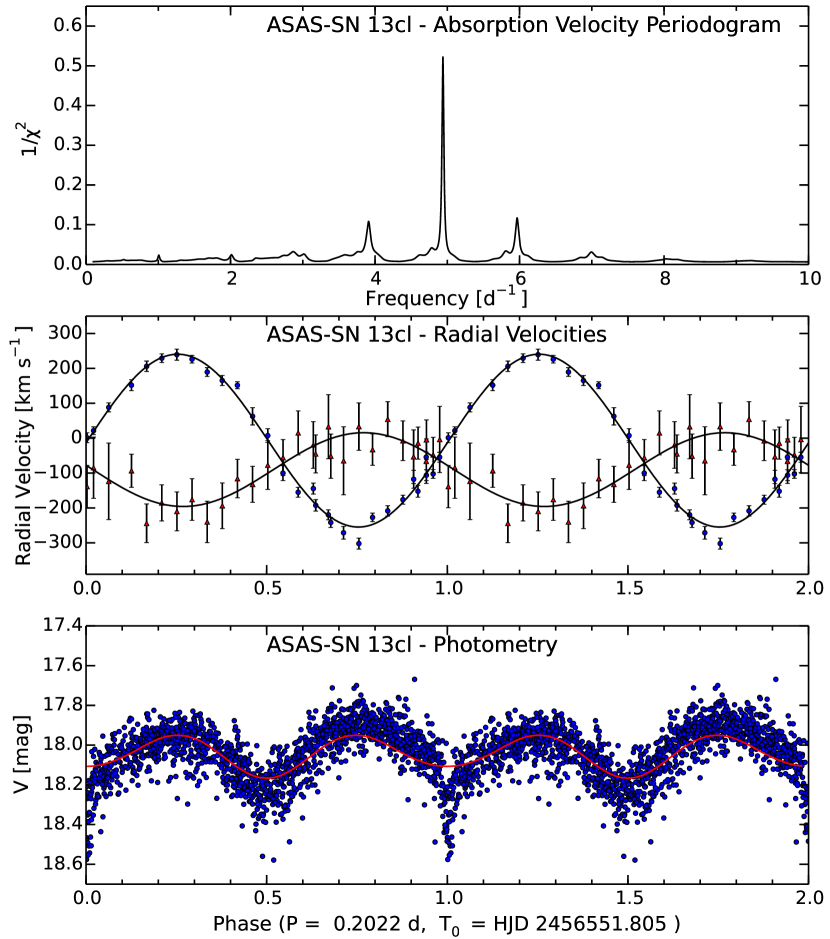
Figure 2: Upper panel: Periodogram of the absorption-line velocities. Middle panel: Absorption velocities (blue circles) and H$\alpha$ (red triangles) emission-line velocities folded on the ephemeris given in the text, with the best-fitting sinusoids superposed. Lower panel: V magnitudes, folded on the same ephemeris as the middle panel. The solid curve is derived from the ellipsoidal variation model described in the text.

To measure the (absorption) radial velocity of the K star, I cross-correlated the spectra against a velocity-compensated sum of many late-type spectra, using the rvsao package (Kurtz & Mink, 1998). The cross-correlation covered from 5100 to 6500 Å, excluding 5800 to 5950 Å to avoid HeI $\lambda$5876 and NaD, which can have an interstellar component. Table 2 gives the velocities. A period search of the resulting timeseries with a ‘residual-gram’ method (Thorstensen et al., 1996) revealed an unambiguous sinusoidal modulation at just under 5 cycle d^-1 (Fig. 2). The H$\alpha$ velocities, measured with a convolution routine, were much noisier than the absorption velocities, but they do show significant modulation consistent with the well-defined absorption period. Table 3 gives parameters sinusoidal fits to the velocities. The velocity modulation of the absorption lines is clearly visible in the lower panel of Fig. 1, which shows a phase-averaged greyscale representation of the spectra.

2.2 Time-series Photometry

The time-series photometry is from an Andor Ikon DU-937N camera mounted on the MDM 1.3m McGraw-Hill telescope, as described in Thorstensen (2013). Individual exposures were 30 s, in the $V$ filter. In each frame, the program star, a comparison star, and two check stars were measured; the main comparison star was 54 arcsec west and 17 arcsec south of the program star. Conditions were generally clear but not photometric, and exposures in which the comparison star’s instrumental magnitude more than $\sim 0.4$ mag fainter than average were excluded from the analysis.

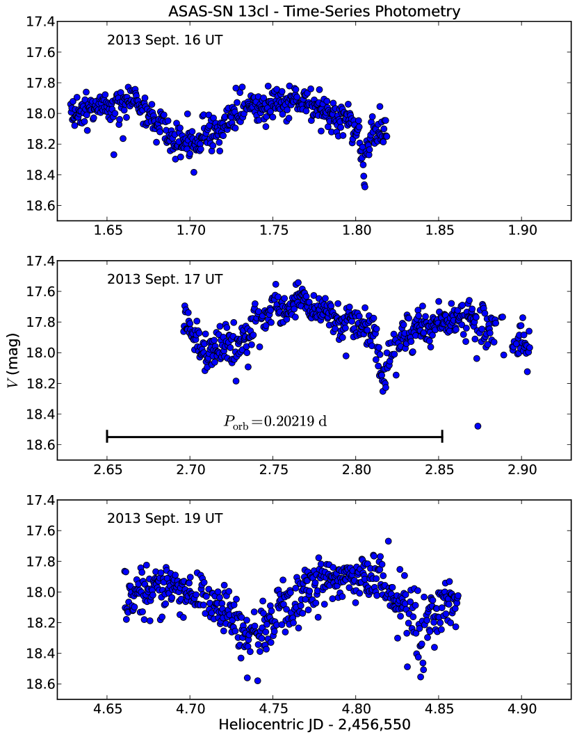
Figure 3: Time series photometry of ASAS-SN 13cl from the McGraw-Hill 1.3m telescope. The magnitudes are relative to the main comparison star, with the estimated $V$ magnitude of the comparison star (15.875) added to set the zero point, The horizontal bar in the middle panel shows the length of the orbital period.

In the SDSS DR10 (Table 1), the program object has $g=18.265$ and $g-r=+0.683$, while the main comparison star has $g=16.194$ and $g-r=+0.545$. Using transformations derived by Robert Lupton, these correspond to $V=17.866$ and $15.875$ respectively. Fig. 3 shows the time series for the three nights, with the zero-point adjusted to approximate $V$ magnitude, and the lower panel of Fig. 2 shows the magnitude plotted against orbital phase.

The photometry shows variation at twice the orbital period, consistent with ellipsoidal modulation. Superposed on this is a sharp dip at inferior conjunction of the secondary, which is apparently a grazing eclipse. The eclipse is clearly visible on the first and second nights, but only just discernible on the third. Table 4 gives the timings of the three eclipses.

2.3 Analysis

Period and Ephemeris. The radial velocities and the grazing eclipses give independent estimates of the period, which agree within their uncertainties. Adopting the weighted mean period yields

$$\hbox{BJD eclipse}=2456551.8052(1)+0.20219(8)E,$$ (1)

where $E$ is an integer.

Masses. The grazing eclipse requires an orbital inclination $i$ not too far from edge-on, and the amplitude of the absorption line velocity variation $K_{\rm abs}$ should reflect the secondary star’s center-of-mass motion with reasonable fidelity. One is less confident of the dynamical interpretation of the H$\alpha$ velocities (see, e.g., Marsh et al. 1987); however, the phase at which they cross their mean velocity is $0.515\pm 0.025$ in the eclipse ephemeris, consistent with the antiphased motion expected if they coincide with the white dwarf. If we take the velocities as reliable for dynamics, we find $q=M_{2}/M_{1}=K_{1}/K_{2}=0.43\pm 0.08$. For $i=75$ degrees, the mass function then implies $0.6{\rm M_{\odot}}<M_{\rm 1}<0.8{\rm M_{\odot}}$ for the white dwarf, and roughly half that for the secondary. As expected, the secondary is undermassive for its spectral type; a recent tabulation by Pecaut and Mamajek (based on Pecaut & Mamajek 2013) estimates 0.7 M_⊙ for typical main-sequence field star at K6, the late (hence low-mass) end of our spectral type range.

Distance. The secondary star’s spectral type constrains its surface brightness, and the Roche lobe geometry combined with the orbital period lets us estimate the secondary’s radius, with only a weak dependence on its mass. The radius and surface brightness yield an absolute magnitude, which together with the observed brightness of the secondary (and an estimated interstellar extinction) yields a distance. All the quantities entering the calculation are uncertain, and some are correlated (e.g., the light fraction attributed to the secondary decreases at cooler spectral types, because the metal lines used in estimating the fraction mostly grow stronger toward cooler types). I therefore used a Monte Carlo procedure to estimate the distance and its uncertainty, which explicitly included the correlation between the secondary’s spectral type and its contribution to the light. For the K$4\pm 2$ secondary, I used magnitudes centered around $V=18.5$, and ranging between extremes of 19.55 (minimum contribution at K6) and 18.10 (maximum contribution at K2). The secondary’s mass (which enters weakly) was taken to be uniformly distributed in the range $0.3\pm 0.15$. The $V$-band surface brightness at each spectral type was computed using a polynomial relation tabulated by Beuermann (2006). I assumed $0.02<E(B-V)<0.18$, guided by the extinction map of Schlegel, Finkbeiner, & Davis (1998), which gives a total extinction of $E(B-V)=0.084$ at this location. The Monte Carlo procedure yielded a median distance of 1180 pc, with a 68-percent confidence range from 990 to 1400 pc.

Ellipsoidal Variation. In favorable cases the light variations of the secondary star can yield useful constraints on system parameters, especially the inclination. To exploit this, Thorstensen & Armstrong (2005) developed a code to model the light variation of a Roche-lobe filling star. ASAS-SN 13cl, unfortunately, is rather too faint and messy for fruitful light-curve fitting, but nonetheless the lower panel of Fig. 2 includes a representative calculation which is useful for comparison. Several features stand out:

1. The sharp dip around phase zero departs significantly from the secondary light curve, indicating that it is very likely an eclipse.

2. The maxima are unequal, with the second hump (phase 0.75) higher than the first. At minimum light dwarf novae often show a pre-eclipse brightening as the ‘hot spot’ where the mass-transfer stream strikes the disk rotates into view (Coppejans et al. 2014 present several examples of this). While this has the correct sense to explain the inequality, the extra light does not persist until eclipse as it does in other systems, so it seems more likely that the secondary’s leading and trailing hemispheres differ in mean brightness.

3. The curve shown has extra light added (assumed constant through the orbit) to approximate the contributions from the rest of the system (accretion disk and so on). This tends to flatten the light curve and push the system to greater computed distances. The amplitude of the computed curve appears to be smaller than that of the data, suggesting that the extra light may have been overestimated; however, it is difficult to justify a smaller contribution on the basis of the spectral decomposition (Fig. 1).

Although the data are noisy and the detailed match imperfect, the modulation’s period and phase confirms that it is mostly ellipsoidal.

3 Discussion

The secondary of ASAS-SN 13cl is warmer than expected. At $P_{\rm orb}=4.85$ h, the temperature discrepancy is not as dramatic as in shorter period systems such as EI Psc Thorstensen et al. (2002a), QZ Ser (Thorstensen et al., 2002b), SDSS J170213.26+322954.1 (Littlefair et al., 2006), and CSS J134052.0+151341 (Thorstensen, 2013), but it is significant.

The recent generation of synoptic sky surveys, most notably the Catalina surveys (Drake et al., 2009), ASAS-SN, and the MASTER survey (Lipunov et al., 2010) have dramatically accelerated the rate of discovery of new dwarf novae (see, e.g., Breedt et al. 2014). The variability criteria favor the discovery of large-amplitude outbursts (Thorstensen & Skinner, 2012). In most CVs with periods less than a few hours, the secondaries are so faint that the systems can become very faint between outbursts, but in systems similar to ASAS-SN 13cl the anomalously bright secondary imposes a ‘floor’ on the total brightness, which can make the amplitude rather modest. In ASAS-SN 13cl, the measured amplitude is less than 3 mag, though it is unlikely to have been caught exactly at maximum. At such relatively small amplitudes, discovery is somewhat more difficult. Also, the known examples of warm-secondary dwarf novae have relatively long inter-outburst times, or have only a single observed outburst. For these reasons, it is likely that a substantial number of these warm-secondary systems await discovery.

Table 1: Properties of ASAS-SN 13cl

Property	Value	Reference
$\alpha_{2000}$	21h 38m 05s.046	SDSS
$\delta_{2000}$	+26${}^{\circ}38^{\prime}19".71$
Outburst date	2013-08-29.35	ASAS-SN
Outburst magnitude	15.66
u	$19.097\pm 0.028$	SDSS
g	$18.265\pm 0.008$
r	$17.582\pm 0.016$
i	$17.287\pm 0.007$
z	$17.055\pm 0.014$
V	17.87
J	$15.137\pm 0.053$	2MASS
H	$14.814\pm 0.063$
K	$14.701\pm 0.079$

Table 2: Radial Velocities

Time	$v$ (absn)	$\sigma$	$v$ (emn)	$\sigma$
	[km s-1]	[km s-1]	[km s-1]	[km s-1]
56546.9338	$-118$	$26$	$-53$	$77$
56546.9408	$-54$	$15$	$-66$	$64$
56548.9009	$-192$	$17$	$-45$	$54$
56548.9093	$-242$	$14$	$-52$	$63$
56549.7790	$-54$	$14$	$-4$	$95$
56549.7875	$22$	$11$	$-85$	$88$
56549.7960	$88$	$13$	$-123$	$110$
56549.8087	$152$	$16$	$-93$	$48$
56549.8172	$206$	$15$	$-244$	$55$
56549.8257	$229$	$12$	$-185$	$52$
56549.8341	$239$	$16$	$-210$	$56$
56549.8426	$226$	$11$	$-176$	$60$
56549.8511	$190$	$12$	$-240$	$59$
56549.8595	$165$	$14$	$-194$	$65$
56549.8680	$152$	$10$	$-116$	$55$
56549.8765	$63$	$25$	$-132$	$52$
56549.8850	$7$	$20$	$-77$	$70$
56549.8935	$-100$	$21$	$-56$	$52$
56549.9020	$-155$	$14$	$15$	$63$
56549.9105	$-144$	$16$	$-19$	$67$
56549.9189	$-220$	$14$	$33$	$92$
56549.9274	$-271$	$18$	$-65$	$97$
56549.9360	$-302$	$16$	$33$	$68$
56550.7524	$-227$	$12$	$-33$	$45$
56550.7609	$-208$	$15$	$54$	$50$
56550.7694	$-176$	$13$	$-7$	$57$
56550.7778	$-152$	$17$	$-14$	$46$
56550.7863	$-102$	$13$	$-48$	$50$
56550.7948	$1$	$14$	$-139$	$61$
56552.8044	$-106$	$15$	$-4$	$57$

Note. — Times given as barycentric Julian dates of mid-integration, minus 2 400 000. The time base is UTC.

Table 3: Fits to Radial Velocities

Description	$T_{0}$	$P$	$K$	$\gamma$	$N$	$\sigma$
	(BJD)	(d)	(km s-1)	(km s-1)		(km s-1)
Absorption	56549.7839(11)	0.20246(20)	246(9)	$-6(6)$	30	20
	56549.7841(12)	[0.20219]	248(9)	$-7(6)$	30	22
H$\alpha$ emission	56549.888(5)	0.2026(9)	105(17)	$-91(12)$	30	40
	56549.888(5)	[0.20219]	106(17)	$-90(12)$	30	40

Note. — Parameters of best-fit sinusoids of the form $v(t)=\gamma+K\sin[2\pi(t-T_{0})/P].$ The epoch $T_{0}$ is expressed as a barycentric Julian day. In the second line for each fit, the period is fixed at the weighted mean derived from the radial velocities and eclipse timings.

Table 4: Eclipse Timings

$E$	Barycentric JD	$\sigma$
0	2456551.8052	0.0003
5	2456552.8164	0.0007
15	2456554.8367	0.0012

Note. — $E$ is an integer cycle count. Times given are barycentric Julian dates of mid-eclipse. The time base is UTC. The last column is the estimated one-sigma uncertainty of the timing, in days.

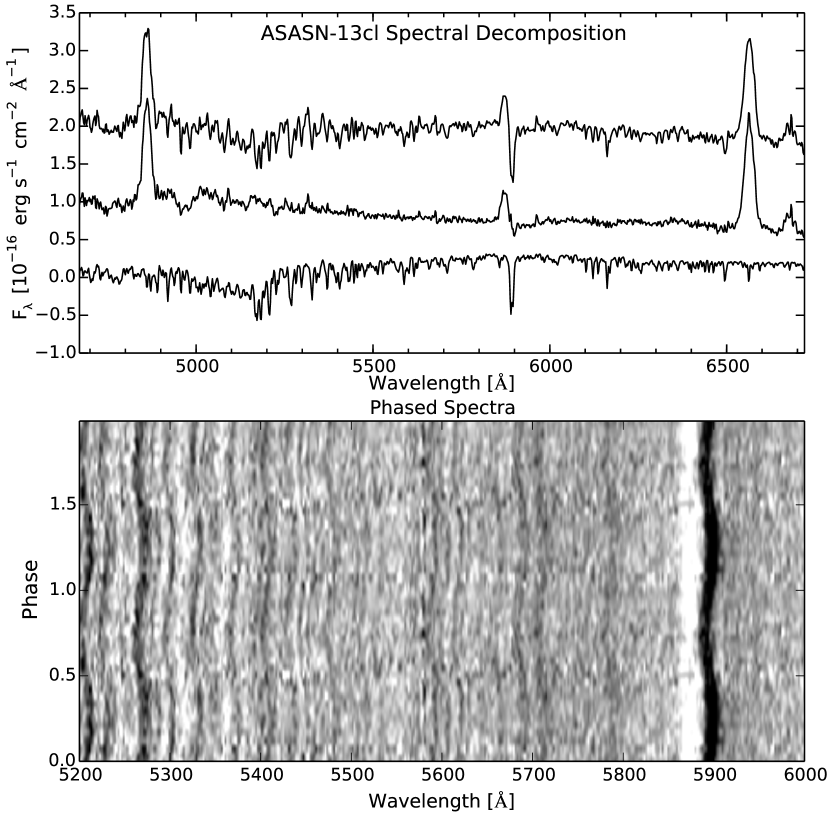
Figure 1: Upper panel: Mean spectrum. The individual spectra were shifted to zero velocity using the absorption-line ephemeris prior to averaging. The middle trace shows the residual after subtracting a scaled spectrum of a K4 star Gliese 570a. The lower trace shows the scaled K4 spectrum that was subtracted; its zero point is shifted downward by one unit to avoid overlap. Lower panel: A greyscale representation the portion of the spectrum from 5200 to 6000 Å. Each line in the image is derived from a running average of the rectified spectra that lie near the nominal orbital phase. The strong absorption line near 5900 Å is NaD, and the emission just blueward of this is HeI $\lambda 5876$.

References

- Marsh et al. (1987) Marsh, T. R., Horne, K., & Shipman, H. L. 1987, MNRAS, 225, 551
- Barrett & Bridgman (2000) Barrett, P. E., & Bridgman, W. T. 2000, in Astronomical Society of the Pacific Conference Proceedings, vol 216, Astronomical Data Analysis Software and Systems IX, ed. N. Manset, C. Veillet, & D. Crabtree , 67
- Beuermann (2006) Beuermann, K. 2006, A&A, 460, 783
- Breedt et al. (2014) Breedt, E., Gänsicke, B. T., Drake, A. J., et al. 2014, MNRAS, 443, 3174
- Coppejans et al. (2014) Coppejans, D. L., Woudt, P. A., Warner, B., et al. 2014, MNRAS, 437, 510
- Covey et al. (2007) Covey, K. R., Ivezić, Ž., Schlegel, D., et al. 2007, AJ, 134, 2398
- Drake et al. (2009) Drake, A. J., et al. 2009, ApJ, 696, 870
- Faulkner et al. (1972) Faulkner, J., Flannery, B. P., & Warner, B. 1972, ApJ, 175, L79
- Gänsicke et al. (2003) Gänsicke, B. T., Szkody, P., de Martino, D., et al. 2003, ApJ, 594, 443
- Hambly et al. (2008) Hambly, N. C., Collins, R. S., Cross, N. J. G., et al. 2008, MNRAS, 384, 637
- Keenan & McNeil (1989) Keenan, P. C., & McNeil, R. C. 1989, ApJS, 71, 245
- Lawrence et al. (2007) Lawrence, A., Warren, S. J., Almaini, O., et al. 2007, MNRAS, 379, 1599
- Lipunov et al. (2010) Lipunov, V., Kornilov, V., Gorbovskoy, E., et al. 2010, Advances in Astronomy, 2010, 349171
- Knigge (2006) Knigge, C. 2006, MNRAS, 373, 484
- Kolb et al. (1998) Kolb, U., King, A. R., & Ritter, H. 1998, MNRAS, 298, L29
- Kurtz & Mink (1998) Kurtz, M. J. & Mink, D. J. 1998, PASP, 110, 934
- Littlefair et al. (2006) Littlefair, S. P., Dhillon, V. S., Marsh, T. R., Gänsicke, B. T. 2006, MNRAS, 371, 1435
- Marsh et al. (1987) Marsh, T. R., Horne, K., & Shipman, H. L. 1987, MNRAS, 225, 551
- Nelemans (2005) Nelemans, G. 2005, in Astronomical Society of the Pacific Conference Series, vol. 330, The Astrophysics of Cataclysmic Variables and Related Objects, ed. J.-M. Hameury & J.-P. Lasota, 27
- Pecaut & Mamajek (2013) Pecaut, M. J., & Mamajek, E. E. 2013, ApJS, 208, 9
- Pickles (1998) Pickles, A. J. 1998, PASP, 110, 863
- Roeser et al. (2010) Roeser, S., Demleitner, M., & Schilbach, E. 2010, AJ, 139, 2440
- Rau et al. (2010) Rau, A., Roelofs, G. H. A., Groot, P. J., et al. 2010, ApJ, 708, 456
- Roelofs et al. (2007) Roelofs, G. H. A., Nelemans, G., & Groot, P. J. 2007, MNRAS, 382, 685
- Schlegel, Finkbeiner, & Davis (1998) Schlegel, D. J., Finkbeiner, D. P., & Davis, M. 1998, ApJ, 500, 525
- Schmidt et al. (2013) Schmidt, S. J., Prieto, J. L., Stanek, K. Z., et al. 2013, arXiv:1310.4515
- Shappee et al. (2012) Shappee, B., Stanek, K., Kochanek, C., et al. 2012, American Astronomical Society Meeting Abstracts #220, 220, #432.03
- Skrutskie et al. (2006) Skrutskie, M. F., Cutri, R. M., Stiening, R., et al. 2006, AJ, 131, 1163
- Thorstensen (2013) Thorstensen, J. R. 2013, PASP, 125, 506
- Thorstensen & Armstrong (2005) Thorstensen, J. R., & Armstrong, E. 2005, AJ, 130, 759
- Thorstensen et al. (2002a) Thorstensen, J. R., Fenton, W. H., Patterson, J. O., et al. 2002a, ApJ, 567, L49
- Thorstensen et al. (2002b) Thorstensen, J. R., Fenton, W. H., Patterson, J., et al. 2002b, PASP, 114, 1117
- Thorstensen et al. (1996) Thorstensen, J. R., Patterson, J., Thomas, G., & Shambrook, A. 1996, PASP, 108, 73
- Thorstensen & Skinner (2012) Thorstensen, J. R., & Skinner, J. N. 2012, AJ, 144, 81
- Warner (1995) Warner, B., in Cataclysmic Variable Stars, 1995, Cambridge University Press, New York
- Witham et al. (2007) Witham, A. R., Knigge, C., Aungwerojwit, A., et al. 2007, MNRAS, 382, 1158
- Woudt et al. (2012) Woudt, P. A., Warner, B., de Budé, D., et al. 2012, MNRAS, 2533