Time-dependent Stochastic Bethe-Salpeter Approach

Abstract

A time-dependent formulation for electron-hole excitations in extended finite systems, based on the Bethe-Salpeter equation (BSE), is developed using a stochastic wave function approach. The time-dependent formulation builds on the connection between time-dependent Hartree-Fock (TDHF) theory and configuration-interaction with single substitution (CIS) method. This results in a time-dependent Schrödinger-like equation for the quasiparticle orbital dynamics based on an effective Hamiltonian containing direct Hartree and screened exchange terms, where screening is described within the Random Phase Approximation (RPA). To solve for the optical absorption spectrum, we develop a stochastic formulation in which the quasiparticle orbitals are replaced by stochastic orbitals to evaluate the direct and exchange terms in the Hamiltonian as well as the RPA screening. This leads to an overall quadratic scaling, a significant improvement over the equivalent symplectic eigenvalue representation of the BSE. Application of the time-dependent stochastic BSE (TDsBSE) approach to silicon and CdSe nanocrystals up to size of $\approx 3000$ electrons is presented and discussed.

I Introduction

Understanding electron-hole excitations in large molecular systems and nanostructures is essential for developing novel optical and electronic devices.Coe, Woo, and Moungi Bawendi (2002); Tessler et al. (2002); Gur et al. (2005); Talapin and Murray (2005) This is due, for example, to the exponential sensitivity of the photo-current characteristics to the excitonic energy levels and the sensitivity of the device performance to the optical oscillator strength. It becomes, therefore, a necessity to develop accurate theoretical tools to describe the excitonic level alignment and the absorption spectrum, with computational complexity that is scalable to systems of experimental relevance (thousands of atoms and more).

There is no doubt that time-dependent density functional theory (TDDFT) Runge and Gross (1984) has revolutionized the field of electronic spectroscopy of small molecular entities.van Leeuwen (2001); Onida, Reining, and Rubio (2002); Maitra et al. (2002); Marques and Gross (2004); Burke, Werschnik, and Gross (2005); Botti et al. (2007); Jacquemin et al. (2009); Casida (2009); Adamo and Jacquemin (2013) TDDFT provides access to excited state energies, geometries, and other properties of small molecules with a relatively moderate computational cost, similar to configuration interaction with single substitutions (CIS) in the linear response frequency-domain formulation Stratmann, Scuseria, and Frisch (1998) ($O\left(N^{4}\right)$, where $N$ is the number of electrons), or even better using a real-time implementation Yabana and Bertsch (1996); Bertsch et al. (2000); Baer and Neuhauser (2004) ($O\left(N^{2}\right)$). In principle TDDFT is exact but in practice approximations have to be introduced. The most common is the so-called time-dependent Kohn-Sham (TDKS) method within the adiabatic approximation, which has been applied to numerous challenging problems Bauernschmitt and Ahlrichs (1996); Bauernschmitt et al. (1998); Fabian (2001); Vasiliev, Ogut, and Chelikowsky (2002); Shao, Head-Gordon, and Krylov (2003); Troparevsky, Kronik, and Chelikowsky (2003); Maitra (2005); Andzelm et al. (2007); Govind et al. (2009); Peach et al. (2009); Kuritz et al. (2011); Peach, Williamson, and Tozer (2011); Srebro et al. (2011); Richard and Herbert (2011); Chantzis et al. (2013); Bauernschmitt et al. (1997); Chelikowsky, Kronik, and Vasiliev (2003); Gavnholt et al. (2009); Hirata and Head-Gordon (1999a); Hirata, Lee, and Head-Gordon (1999); Jacquemin et al. (2008); Stein, Kronik, and Baer (2009a, b); Phillips et al. (2011); Ou et al. (2014) with great success. However, TDKS often fails,Parac and Grimme (2003); Grimme and Parac (2003); Dreuw and Head-Gordon (2004); Maitra et al. (2004); Hieringer and Görling (2006); Levine et al. (2006); Lopata et al. (2011); Kowalczyk, Yost, and Van Voorhis (2011); Isborn et al. (2013) particularly for charge-transfer excited states, multiple excitations, and avoided crossings. In the present context, perhaps the most significant failure of TDKS is in the description of low-lying excitonic states in bulk.Albrecht et al. (1998); Rohlfing and Louie (2000); Sottile et al. (2007); Ramos et al. (2008); Rocca et al. (2012)

An alternative to TDDFT, which has mainly been applied to condensed periodic structures, is based on many-body perturbation theory (MBPT). The most common flavors are the GW approximation Hedin (1965) to describe quasiparticle excitations ($G$ indicates the single-particle Green function and $W$ the screened Coulomb interaction) and the Bethe-Salpeter equation (BSE) Salpeter and Bethe (1951) to describe electron-hole excitations. Both approaches offer a reliable solution to quasiparticle Hybertsen and Louie (1985, 1986); Steinbeck et al. (1999); Rieger et al. (1999); Rinke et al. (2005); Neaton, Hybertsen, and Louie (2006); Tiago and Chelikowsky (2006); Friedrich and Schindlmayr (2006); Gruning, Marini, and Rubio (2006); Shishkin and Kresse (2007); Huang and Carter (2008); Rostgaard, Jacobsen, and Thygesen (2010); Tamblyn et al. (2011); Liao and Carter (2011); Refaely-Abramson, Baer, and Kronik (2011); Marom et al. (2012); Isseroff and Carter (2012); Refaely-Abramson et al. (2012); Kronik et al. (2012) and optical Albrecht et al. (1998); Benedict, Shirley, and Bohn (1998); Rohlfing and Louie (2000); Benedict et al. (2003); Spataru et al. (2004); Tiago and Chelikowsky (2006); Sai et al. (2008); Fuchs et al. (2008); Ramos et al. (2008); Palummo et al. (2009); Schimka et al. (2010); Rocca, Lu, and Galli (2010); Blase and Attaccalite (2011); Rocca et al. (2012); Faber et al. (2012, 2014) excitations, even for situations where TDKS often fails, for example in periodic systems Albrecht et al. (1998); Benedict, Shirley, and Bohn (1998); Rohlfing and Louie (2000); Sottile et al. (2007); Ramos et al. (2008); Rocca et al. (2012) or for charge-transfer excitations in molecules.Rocca, Lu, and Galli (2010) However, the computational cost of the MBPT methods is considerably more demanding than for TDKS, because conventional techniques require the explicit calculation of a large number of occupied and virtual electronic states and the evaluation of a large number of screened exchange integrals between valence and conduction states. This leads to a typical scaling of $O\left(N^{6}\right)$ and limits the practical applications of the BSE to small molecules or to periodic systems with small unit cells.

Significant progress has been made by combining ideas proposed in the context of TDDFT Walker et al. (2006); Rocca et al. (2008) and techniques used to represent the dielectric function Wilson, Gygi, and Galli (2008) based on density functional perturbation theory.Baroni et al. (2001) This leads to an approach that explicitly requires only the occupied orbitals (and not the virtual states) and thus scales as $O\left(N^{2}\times N_{k}^{2}\times N_{g}\right)$,Rocca et al. (2012) where $N_{k}$ the number of points in the Brillouin zone and $N_{g}$ the size of the basis. Even with this more moderate scaling, performing a Bethe-Salpeter (BS) calculation for large systems with several thousands of electrons is still prohibitive.

Recently, we have proposed an alternative formulation for a class of electronic structure methods ranging from the density functional theory (DFT),Baer, Neuhauser, and Rabani (2013); Neuhauser, Baer, and Rabani (2014) Møller-Plesset second order perturbation theory (MP2),Neuhauser, Rabani, and Baer (2013a); Ge et al. (2013) the random phase approximation (RPA) to the correlation energy,Neuhauser, Rabani, and Baer (2013b) and even for multiexciton generation (MEG).Baer and Rabani (2012) But perhaps the most impressive formulations are that for calculating the quasiparticle energy within the GW many-body perturbation correction to DFT Neuhauser et al. (2014) and for a stochastic TDDFT.Gao et al. (2015) The basic idea behind our formulation is that the occupied and virtual orbitals of the Kohn-Sham (KS) Hamiltonian are replaced by stochastic orbitals and the density and observables of interest are determined from an average of stochastic replicas in a trace formula. This facilitates “self-averaging” which leads to the first ever report of sublinear scaling DFT electronic structure method (for the total energy per electron) and nearly linear scaling GW approach, breaking the theoretical scaling limit for GW as well as circumventing the need for energy cutoff approximations.

In this paper we develop an efficient approach for calculating electron-hole excitations (rather than charge excitations) based on the BSE, making it a practical and accessible computational tool for very large molecules and nanostructures. The BSE is often formulated in the frequency domain and thus requires the calculation of screened exchange integrals between occupied and virtual states. Instead, we introduce concepts based on stochastic orbitals and reformulate the BSE in the time-domain as means of reducing CPU time and memory. The real-time formulation of the BSE delivers the response function (and thus the optical excitation spectrum) without requiring full resolution of the excitation energies, thereby reducing dramatically the computational cost. This is demonstrated for well-studied systems of silicon and CdSe nanocrystals, covering the size range of $N\approx 100-3000$ electrons. Within this range, we show that the approach scales quadratically ($O\left(N^{2}\right)$) with system size.

II Theory

In this section we review the symplectic eigenvalue formulation of the BSE and then build on the connections between configuration interaction with single substitution (CIS) and time-dependent Hartree-Fock (TDHF) to formulate a time-dependent wave-equation for the BSE.

II.1 Symplectic Eigenvalue Bethe-Salpeter Equation

Within linear response, one can show that the BSE is equivalent to solving the symplectic eigenvalue problem Casida (1995, 1996); Furche (2001)

$${\cal L}\left(\begin{array}[]{c}X\\ Y\end{array}\right)=\hbar\omega\left(\begin{array}[]{cc}1&0\\ 0&-1\end{array}\right)\left(\begin{array}[]{c}X\\ Y\end{array}\right)$$ (1)

where

$${\cal L}=\begin{pmatrix}A&B\\ -B&-A\end{pmatrix}$$ (2)

with

$$A =D+2K^{X}+K^{D}$$

$$B =2K^{X}+K^{D}.$$ (3)

The diagonal ($D$), exchange ($K^{x}$) and direct ($K^{d}$) terms are given by (we use $i,j,\mbox{ and $k\dots$}$ as occupied (hole) state indices, $a,b,\mbox{ and }c\dots$ as unoccupied (electron) states indices, and $r,s,\mbox{ and }t\dots$ for general indices):

$$D_{ia,bj}= \left(\varepsilon_{a}-\varepsilon_{i}\right)\delta_{ab}\delta_{ij}$$ (4)

$$K_{ia,bj}^{X}= \langle\phi_{a}\phi_{i}|\hat{v}_{C}|\phi_{b}\phi_{j}\rangle=\iint d\mathbf{r}d\mathbf{r}^{\prime}$$

$$\times \phi_{i}\left(\mathbf{r}\right)\phi_{a}\left(\mathbf{r}\right)v_{C}\left(\left|{\bf r}-{\bf r}^{\prime}\right|\right)\phi_{j}\left(\mathbf{r}^{\prime}\right)\phi_{b}\left(\mathbf{r}^{\prime}\right)$$ (5)

$$K_{ia,bj}^{D}= \langle\phi_{a}\phi_{b}|\hat{W}|\phi_{i}\phi_{j}\rangle=\iint d\mathbf{r}d\mathbf{r}^{\prime}$$

$$\times \phi_{b}\left(\mathbf{r}\right)\phi_{a}\left(\mathbf{r}\right)W\left(\mathbf{r},\mathbf{r}^{\prime},0\right)\phi_{j}\left(\mathbf{r}^{\prime}\right)\phi_{i}\left(\mathbf{r}^{\prime}\right).$$ (6)

Here, $\varepsilon_{a}$ and $\varepsilon_{i}$ are the quasi-particle energies for the virtual and occupied space (which can be obtained from a DFT+GW calculation or from an alternative suitable approach) and $\phi_{a}\left({\bf r}\right)$ and $\phi_{i}\left({\bf r}\right)$ are the corresponding quasi-particle orbitals; $\hat{v}_{C}$ is the Coulomb potential while $W$ is the screened Coulomb potential, typically calculated within the Random Phase Approximation (RPA), which can be written in real space as:

$$W\left(\mathbf{r},\mathbf{r}^{\prime},0\right)=v_{C}\left(\left|{\bf r}-{\bf r}^{\prime}\right|\right)+\delta W^{RPA}\left(\mathbf{r},\mathbf{r}^{\prime},0\right),$$ (7)

with

$$\delta W^{RPA}\left(\mathbf{r},\mathbf{r}^{\prime},0\right)= \iint d\mathbf{r}^{\prime\prime}d\mathbf{r}^{\prime\prime\prime}v_{C}\left(\left|{\bf r}-\mathbf{r}^{\prime\prime}\right|\right)$$

$$\tilde{\chi}^{RPA}\left({\bf\mathbf{r}}^{\prime\prime},{\bf r}^{\prime\prime\prime},0\right) \left(v_{C}\left(\left|{\bf r}^{\prime\prime\prime}-{\bf r}^{\prime}\right|\right)+f_{XC}\mbox{$\left(\mathbf{r}^{\prime\prime\prime}\right)$}\delta\mbox{$\left({\bf r}^{\prime\prime\prime}-{\bf r}^{\prime}\right)$}\right).$$ (8)

Here, $f_{XC}\mbox{$\left(\mathbf{r}\right)$}$ is the DFT exchange-correlation potential (if DFT is used to obtain the RPA screening, otherwise set $f_{XC}\mbox{$\left(\mathbf{r}\right)$}=0$), and $\tilde{\chi}^{RPA}\left({\bf r},{\bf r}^{\prime},0\right)$ is the half-Fourier transform (at $\omega=0$) of the real-time density-density correlation function within the RPA (the latter can be also obtained from TDDFT, as further discussed below). We note in passing that often the above is solved within the Tamm-Dancoff approximation (TDA),Dyson (1953); Taylor (1954) which sets $B=0$ and thus only requires the diagonalization of the matrix $A$.

II.2 Time-Dependent Bethe-Salpeter Equation (TDBSE)

The time-dependent formulation of the BSE follows from the connections made between CIS and TDHF.Casida (1995, 1996); Hirata and Head-Gordon (1999b); Hirata, Head-Gordon, and Bartlett (1999) In short, solving the TDHF equations $i\hbar\frac{\partial\phi_{j}\left({\bf r},t\right)}{\partial t}=\hat{h}_{HF}\left(t\right)\phi_{j}\left({\bf r},t\right)$ for the occupied orbitals is identical to solving the symplectic eigenvalue problem of Eq. (1) with $\delta W\left(\mathbf{r},\mathbf{r}^{\prime},0\right)=0$. Here, $\hat{h}_{HF}=\hat{t}+\hat{v}_{ion}+\hat{v}_{H}\left(t\right)+\hat{k}_{X}\left(t\right)$ is the Hartree-Fock (HF) Hamiltonian, $\hat{t}$ is the kinetic energy, $\hat{v}_{ion}$ is the external potential, $\hat{v}_{H}\psi\left(\mathbf{r}\right)=\int d\mathbf{r}^{\prime}v_{C}\left(\left|{\bf r}-{\bf r}^{\prime}\right|\right)n\left({\bf r}^{\prime},t\right)\psi\left(\mathbf{r}\right)$ is the Hartree potential, and $\hat{k}_{X}\left(t\right)\psi\left(\mathbf{r}\right)=-\frac{1}{2}\int d\mathbf{r}^{\prime}\rho\left(\mathbf{r},{\bf r}^{\prime},t\right)v_{C}\left(\left|{\bf r}-{\bf r}^{\prime}\right|\right)\psi\left(\mathbf{r^{\prime}}\right)$ is the non-local exchange potential. $n\left({\bf r},t\right)=2\sum_{j}\left|\phi_{j}\left({\bf r},t\right)\right|^{2}$ and $\rho\left(\mathbf{r},{\bf r}^{\prime},t\right)=2\sum_{j}\phi_{j}^{*}\left({\bf r^{\prime}},t\right)\phi_{j}\left({\bf r},t\right)$ are the time-dependent electron density and density matrix, respectively. The connection to CIS is made by realizing that for $\delta W\left(\mathbf{r},\mathbf{r}^{\prime},0\right)=0$ and setting $B=0$ (the TDA), the symplectic eigenvalue problem of Eq. (1) is nothing else but the CIS Hamiltonian. Thus, TDHF within the TDA and CIS are identical.

We follow a similar logic and derive an adiabatic time-dependent BSE:

$$i\hbar\frac{\partial\phi_{j}^{\gamma}\left({\bf r},t\right)}{\partial t}=\hat{h}_{BS}^{\gamma}\left(t\right)\phi_{j}^{\gamma}\left({\bf r},t\right)$$ (9)

where $\gamma$ is a perturbation strength (i.e., $\gamma=0$ is the unperturbed case, see Eq. (12)) with a screened effective Hamiltonian given by:

$$\hat{h}_{BS}^{\gamma}=\hat{h}_{qp}+\hat{v}_{H}^{\gamma}\left(t\right)-\hat{v}_{H}^{0}\left(t\right)+\hat{k}_{\epsilon X}^{\gamma}\left(t\right)-\hat{k}_{\epsilon X}^{0}\left(t\right).$$ (10)

Here, $\hat{h}_{qp}$ is the quasi-particle Hamiltonian which is typically determined from a GW calculation correcting the quasiparticle energies and orbitals of the underlying DFT. The GW approximation to $\hat{h}_{qp}$ is rather difficult to implement since it involves a non-local, energy-dependent operator. An alternative is to use a DFT approach that provides an accurate description of quasiparticle excitations.Baer and Neuhauser (2005); Brothers et al. (2008) However, since the exact model for $\hat{h}_{qp}$ is not the central target of the present work, we represent it by a simple semi-empirical local Hamiltonian of the form:Wang and Zunger (1994a, 1995, 1996); Fu and Zunger (1997a); Williamson and Zunger (2000); Franceschetti and Zunger (2000a); Zunger (2001)

$$\hat{h}_{qp}\approx\hat{t}+\hat{v}_{ps},$$ (11)

where, as before $\hat{t}$ is the kinetic energy and $\hat{v}_{ps}=\sum_{\alpha}\hat{v}_{\alpha}$ is the empirical pseudopotential, given as a sum of atomic pseudopotentials which were generated to reproduce the bulk band structure, providing accurate quasi-particle excitations in the bulk. The semiempirical approach has been successfully applied to calculate the quasi-particle spectrum of semiconducting nanocrystals of various sizes and shapes.Wang and Zunger (1994a, 1996); Fu and Zunger (1997b); Rabani et al. (1999); Reboredo, Franceschetti, and Zunger (2000); Franceschetti and Zunger (2000a, b); Eshet, Grünwald, and Rabani (2013)

In Eq. (10), $\hat{v}_{H}^{\gamma}\left(t\right)\psi\left(\mathbf{r}\right)=\int d\mathbf{r}^{\prime}v_{C}\left(\left|{\bf r}-{\bf r}^{\prime}\right|\right)n^{\gamma}\left({\bf r}^{\prime},t\right)\psi\left(\mathbf{r}\right)$ is the Hartree potential with $n^{\gamma}\left({\bf r},t\right)=2\sum_{j}\left|\phi_{j}^{\gamma}\left({\bf r},t\right)\right|^{2}$ and $\hat{k}_{\epsilon X}^{\gamma}\left(t\right)\psi\left(\mathbf{r}\right)=-\frac{1}{2}\int d\mathbf{r}^{\prime}\rho^{\gamma}\left(\mathbf{r},{\bf r}^{\prime},t\right)W^{RPA}\left({\bf r},{\bf r}^{\prime},0\right)\psi\left(\mathbf{r^{\prime}}\right)$ is the screened exchange potential with $W^{RPA}\left({\bf r},{\bf r}^{\prime},0\right)$ given by Eqs. (7) and (8) and $\rho^{\gamma}\left(\mathbf{r},{\bf r}^{\prime},t\right)=2\sum_{j}\phi_{j}^{\gamma}\left({\bf r^{\prime}},t\right)^{*}\phi_{j}^{\gamma}\left({\bf r},t\right)$. The application of $\hat{k}_{\epsilon X}^{\gamma}\psi\left(\mathbf{r}\right)$ is further discussed below.

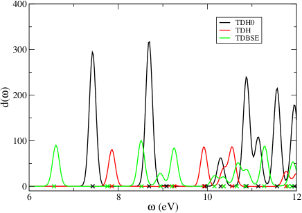
Figure 1: Comparison of BS calculations using the symplectic eigenvalue (Eq. (2), $x$-symbols) with the frequency dependent dipole-dipole correlation generated from TDBSE (Eqs. (10), (9) and (11), solid lines) for $\mbox{SiH}_{4}$. Black: TDBSE with $\gamma=0$ (TDH0) compared with eigenvalues of Eq. (2) setting $K^{X}$ and $K^{D}$ to zero. Red: TDBSE with $\hat{h}_{BS}^{\gamma}=\hat{h}_{qp}+\hat{v}_{H}^{\gamma}\left(t\right)-\hat{v}_{H}^{0}\left(t\right)$ (TDH) compared with Eq. (2) setting $K^{d}$ to zero (TDH). Green: TDBSE with $\gamma=10^{-5}$au (TDBSE) compared with Eq. (2), both for $\epsilon=5$.

In analogy with the relations derived between TDHF and its eigenvalue representation, it is clear that the time-dependent formulation for the BSE given by Eqs. (9) and (10) is identical to the full symplectic eigenvalue problem of Eq. (1). In Fig. 1 we compare the results for $\mbox{SiH}_{4}$ on a $8\times 8\times 8$ grid generated by propagating the occupied orbitals with the Bethe-Salpeter Hamiltonian (10) (TDBSE) to the exact diagonalization of Eq. (2) (static approach). We use a local semi-empirical pseudopotential that has been applied successfully to study the optical properties of silicon nanocrystals.Wang and Zunger (1994a, b); Zunger and Wang (1996) For both the direct approach and the TDBSE we approximate $W\left({\bf r},{\bf r}^{\prime},0\right)$ by $\epsilon^{-1}v_{C}\left(\left|{\bf r}-{\bf r}^{\prime}\right|\right)$, where $\epsilon$ is a constant screening parameter. The idea is to confirm that the eigenvalues of Eq. (2) and the time-dependent version of the BSE are identical (validating both the theory and the implementation).

The time-domain calculations are based on a linear-response approach to generate the dipole-dipole correlation function $d\left(t\right)$ and its Fourier transform $\tilde{d}\left(\omega\right)=\int_{0}^{\infty}dt\,e^{i\omega t}d\left(t\right)$. In short, we perturb the occupied eigenstates ($\phi_{j}\left(\mathbf{r}\right)$) of $\hat{h}_{qp}$ at $t=0$:

$$\phi_{j}^{\gamma}\left({\bf r},t=0\right)=e^{-i\gamma z/\hbar}\phi_{j}\left({\bf r}\right),$$ (12)

where for simplicity, we assume that the dipole is in the $z$–direction. We then propagate these orbitals according to Eq. (9) and generate the dipole-dipole correlation function:

$$d\left(t\right)=\frac{1}{\gamma}\int d\mathbf{r}\,z\left(n^{\gamma}\left({\bf r},t\right)-n^{0}\left({\bf r},t\right)\right),$$ (13)

where as before $n^{\gamma}\left({\bf r},t\right)=2\sum_{j}\left|\phi_{j}^{\gamma}\left({\bf r},t\right)\right|^{2}$and $\gamma$ is a small parameter representing the strength of the perturbation, typically $10^{-3}-10^{-5}\hbar E_{h}^{-1}$.

The agreement for the position of the excitations (solid lines) generated by the time-domain BSE is perfect with the static calculation ($x$-symbols), as seen in Fig. 1. The resolved individual transitions are broadened reflecting the finite propagation time used for the time-domain calculations. We find that in some cases the oscillator strength is very small and thus a transition is not observed in $\tilde{d}\left(\omega\right)$.

An additional important test of the TDBSE formalism is whether the Hamiltonian in Eq. (10) preserves the Ehrenfest theorem (see Appendix B for more details). Naturally, this would be the case if $\hat{h}_{qp}$ would include the terms $\hat{v}_{H}^{0}\left(t\right)$ and $\hat{k}_{\epsilon X}^{0}\left(t\right)$, such that they cancel out for $\hat{h}_{BS}^{\gamma}.$ However, for an arbitrary choice of $\hat{h}_{qp}$ this needs to be confirmed. In Figure 2 we plot the average momentum for $\mbox{SiH}_{4}$ calculated in two different ways. The solid curves were obtained directly from:

$$\frac{\left\langle\mathbf{p}\left(t\right)\right\rangle}{m}=-2i\hbar\sum_{j}\int d\mathbf{r}\phi_{j}^{\gamma}\left(\mathbf{r},t\right)^{*}\frac{\partial}{\partial\mathbf{r}}\phi_{j}^{\gamma}\left(\mathbf{r},t\right),$$ (14)

while the dashed curves were obtained by taking the numerical time derivative (central difference) of the expectation value of $\mathbf{r}\left(t\right):$

$$\frac{\left\langle\mathbf{p}\left(t\right)\right\rangle}{m}=\frac{\partial}{\partial t}\left\langle\mathbf{q}\left(t\right)\right\rangle=2\frac{\partial}{\partial t}\sum_{j}\int d\mathbf{r}\phi_{j}^{\gamma}\left(\mathbf{r},t\right)^{*}\mathbf{q}\phi_{j}^{\gamma}\left(\mathbf{r},t\right).$$ (15)

The agreement is not perfect but improves with decreasing the time step $\delta t$ (not shown here). We also show the results for the time-dependent Hartree (TDH), i.e., ignoring the screened exchange term in $\hat{h}_{BS}^{\gamma}$. The deviations observed for TDBSE and TDH are similar, although for TDH the Ehrenfest theorem holds exactly and thus the agreement should be perfect. The difference are associated with numerical inaccuracies resulting from the finite time step and grid used in the calculation. The inset shows that the deviations are insignificant even at much longer times over many periods.

Figure 2: Average momentum along the $z$-direction calculated in two ways (see text for more details) for $\mbox{SiH}_{4}$ using the TDH (black curves) and the TDBSE (red curves) methods. Solid and dashed curves where generated using the expectation value of the momentum (Eq. (14)) and the numerical derivative of the expectation value of the position (Eq. (15)), respectively. Inset: same for longer times.

III Time-Dependent Stochastic Bethe-Salpeter Equation

We consider two formulations for the time-dependent stochastic BSE (TDsBSE). The first approach is a direct generalization of the approach we have recently developed for the stochastic TDH,Gao et al. (2015) in which we describe an efficient way to account for the the screened exchange term in the $\hat{h}_{BS}^{\gamma}$. This approach works well for short times, however, unlike in TDH, the inclusion of an exchange term requires an increasing number of stochastic orbitals with the system size. The second approach offers access to timescales relevant for most spectroscopic applications at a practical quadratic computational cost.

III.1 Extending the Stochastic TDH to Include a Screened Exchange Term

We limit the discussion, in the body of this paper, to the case where $W\left({\bf r},{\bf r}^{\prime},0\right)$ is replaced by $\epsilon^{-1}v_{C}\left(\left|{\bf r}-{\bf r}^{\prime}\right|\right)$, where $\epsilon$ is a function of $\left|{\bf r}-{\bf r}^{\prime}\right|$. The algorithm for the TDsBSE is based on the following steps:

1. Generate $N_{\zeta}$ stochastic orbitals $\zeta_{j}\left({\bf r}\right)=e^{i\theta_{j}\left({\bf r}\right)}/\sqrt{\delta V}$, where $\theta_{j}\left({\bf r}\right)$ is a uniform random variable in the range $\left[0,2\pi\right]$ at each grid point (total of $N_{g}$ grid points), $\delta V$ is the volume element of the grid, and $j=1\,,\dots,\,N_{\zeta}$. The stochastic orbitals obey the relation $\mathbf{1}=\left<\left|\zeta\left\rangle\right\langle\zeta\right|\right>_{\zeta}$ where $\left<\cdots\right>_{\zeta}$ denotes a statistical average over $\zeta$.

2. Project each stochastic orbital $\zeta_{j}\left({\bf r}\right)$ onto the occupied space: $\left|\xi_{j}\right\rangle\equiv\sqrt{\theta_{\beta}\left(\mu-\hat{h}_{qp}\right)}\left|\zeta_{j}\right\rangle$, where $\theta_{\beta}\left(x\right)=\frac{1}{2}\mbox{erfc}\left(\beta\left(x\right)\right)$ is a smooth representation of the Heaviside step function Baer, Neuhauser, and Rabani (2013) and $\mu$ is the chemical potential. The action of $\sqrt{\hat{\theta}_{\beta}}$ is performed using a suitable expansion in terms of Chebyshev polynomials in the static quasi-particle Hamiltonian with coefficients that depend on $\mu$ and $\beta$.Kosloff (1988)

3. Define non-perturbed and perturbed orbitals for $t=0$ to the orbitals: $\xi_{j}^{0}\left({\bf r},t=0\right)=\xi_{j}\left({\bf r}\right)$, $\xi_{j}^{\gamma}\left({\bf r},t=0\right)=e^{-iv\left({\bf r}\right)/\hbar}\xi_{j}\left({\bf r}\right)$. For the absorption spectrum, the perturbation is given by $v\left(\mathbf{r}\right)=r_{\alpha}$ and $\alpha\equiv x,y,z$.

4. Propagate the perturbed ($\xi_{j}^{\gamma}\left({\bf r},t\right)$) and unperturbed ($\xi_{j}^{0}\left({\bf r},t\right)$) orbitals according to the adiabatic time-dependent BSE:

   $$i\hbar\frac{\partial\xi_{j}^{\gamma}\left({\bf r},t\right)}{\partial t} =\hat{h}_{BS}^{\gamma}\left(t\right)\xi_{j}^{\gamma}\left({\bf r},t\right).$$ (16)

   Use the split operator technique to perform the time propagation from time $t$ to time $t+\Delta t$:

   $$e^{-\frac{i}{\hbar}\hat{h}_{BS}^{\gamma}\Delta t} \approx e^{-\frac{i}{2\hbar}\left(\hat{v}_{ps}+\hat{v}_{H}^{\gamma}\left(t\right)-\hat{v}_{H}^{0}\left(t\right)\right)\Delta t}$$

   $$\times e^{-\frac{i}{2\hbar}\hat{t}\Delta t}e^{-\frac{i}{\hbar}\left(\hat{k}_{\epsilon X}^{\gamma}\left(t\right)-\hat{k}_{\epsilon X}^{0}\left(t\right)\right)\Delta t}$$

   $$\times e^{-\frac{i}{2\hbar}\hat{t}\Delta t}e^{-\frac{i}{2\hbar}\left(\hat{v}_{ps}+\hat{v}_{H}^{\gamma}\left(t\right)-\hat{v}_{H}^{0}\left(t\right)\right)\Delta t}$$ (17)

   where propagator step involving the non-local screened exchange is applied using a Taylor series (in all applications below we stop at ):

   $$e^{-\frac{i}{\hbar}\left(\hat{k}_{\epsilon X}^{\gamma}\left(t\right)-\hat{k}_{\epsilon X}^{0}\left(t\right)\right)\Delta t} \approx$$

   $$1- \frac{i}{\hbar}\left(\hat{k}_{\epsilon X}^{\gamma}\left(t\right)-\hat{k}_{\epsilon X}^{0}\left(t\right)\right)\Delta t+\cdots$$ (18)

5. The application of $\hat{h}_{BS}^{\gamma}\left(t\right)$ is done as follows:

   1. The kinetic energy is applied using a Fast Fourier Transform (FFT).

   2. The Hartree term is generated using convolution and FFT with the density obtained from the stochastic orbitals:

      $$n^{\gamma}\left({\bf{\bf r}},t\right) =\frac{2}{N_{\zeta}}\sum_{j=1}^{N_{\zeta}}\left|\xi_{j}^{\gamma}\left({\bf r},t\right)\right|^{2}.$$ (19)

   3. The time-consuming part of the application of $\hat{h}_{BS}^{\gamma}$ on a vector $\psi$ in Hilbert space is $\hat{k}_{\epsilon X}^{\gamma}\left(t\right)-\hat{k}_{\epsilon X}^{0}\left(t\right)$. This operation scales as $O\left(NN_{grid}\right)$ and one needs to carry this for all occupied states, leading a $O\left(N^{2}N_{grid}\right)$ computational scaling. To reduce this high scaling resulting from the exchange operation we use the same philosophy underlying this work, i.e., replacing summation with stochastic averaging. In practice we therefore replace the summation over occupied orbitals in the exchange operation by acting with very few $n_{\eta}\ll N_{\zeta}$, typically $n_{\eta}=1-16,$ stochastic orbitals write the exchange operation as:

      $$\hat{k}_{\epsilon X}^{\gamma}\left(t\right)\psi\left(\mathbf{r},t\right) =\frac{1}{n_{\eta}}\sum_{x=1}^{n_{\eta}}\eta_{x}^{\gamma}\left(\mathbf{r},t\right)$$

      $$\times\mbox{$\int$d{r}}^{\prime}\epsilon^{-1} v_{C}\left(\left|{\bf r}-{\bf r}^{\prime}\right|\right)\eta_{x}^{\gamma}\left(\mathbf{r}^{\prime},t\right)^{*}\psi\left(\mathbf{r}^{\prime},t\right).$$ (20)

      The key is that these stochastic orbitals are defined as a different random combination of the full set of orbitals at any given time step$\eta_{x}^{\gamma}$ are defined as random superpositions of the $N_{\zeta}$ stochastic orbitals:

      $$\eta_{x}^{\gamma}\left(\mathbf{r},t\right) =\frac{1}{N_{\zeta}}\sum_{j}^{N_{\zeta}}e^{i\alpha_{xj}(t)}\xi_{j}^{\gamma}\left({\bf r},t\right).$$ (21)

      To improve the representation of the stochastic exchange operators, the random phases $\alpha_{xj}\left(t\right)$ are re-sampled at each time step. Note that the same phases are used for both $\eta_{x}^{\gamma}\left(\mathbf{r},t\right)$ and $\eta_{x}^{0}\left(\mathbf{r},t\right)$. This use of stochastic orbitals reduces the overall scaling of the method to quadratic, since $n_{\eta}$ does not dependent on the system size.

In Fig. 3 we show the calculated $d\left(t\right)$ and $S\left(t\right)=\int_{0}^{t}ds\,d\left(s\right)^{2}$ for a series of silicon nanocrystals. We used $n_{\zeta}=16$ which leads to results that are indistinguishable from $n_{\zeta}=N_{\zeta}$ (though even a smaller $n_{\zeta}$would have been sufficient). We used a constant value for$\epsilon=5$ and the time step was $\Delta t=0.025\mbox{au}$.

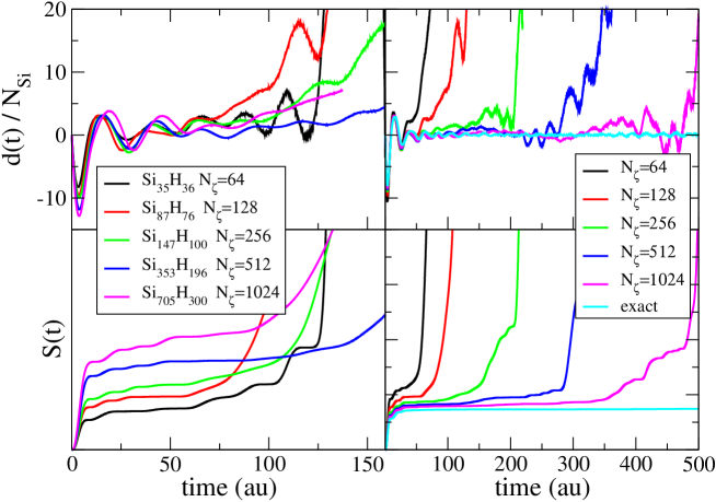
Figure 3: Upper left: Dipole-dipole correlation function (Eq. (13)) normalized to the number of silicon atoms in the nanocrystal ($N_{Si}$) for several nanocrystals sizes. For each size we use a different number of stochastic orbitals. Lower left: Integrate dipole-dipole correlation $S\left(t\right)=\int_{0}^{t}ds\,d\left(s\right)^{2}$. The onset of divergence scales roughly linearly with the size. Upper right: Dipole-dipole correlation function normalized to the number of silicon atoms for $\mbox{Si}_{87}\mbox{H}_{76}$ for different values of $N_{\zeta}$. Lower right: Corresponding values for $S\left(t\right)$.

In general, we find that the results converge up to a time $\tau_{C}$ and then the signal diverges exponentially. Several conclusions can be drawn from these calculations:

1. The stochastic approximation to $d\left(t\right)$ oscillates about zero up to a time $\tau_{C}$, but this is followed by a gradual increase which eventually leads to divergence (upper panels of Fig. 3).

2. $\tau_{C}$ increases with the number of stochastic orbitals, $N_{\zeta}$, roughly as $\tau_{C}\propto N_{\zeta}^{\alpha}$ with $\alpha=1-2$ (right panels of Fig. 3). This is somewhat better than the case for TDH for which $\tau_{C}$ roughly scaled as $N_{\zeta}^{1/2}$.

3. $\tau_{C}$ decreases with increasing system size roughly as $\frac{1}{N_{e}}$, where $N_{e}$ is the number of electrons (left panels of Fig. 3). Therefore, to converge the results to a fixed $\tau_{C}$ one has to increase $N_{\zeta}$ roughly linearly with the system size . This leads to a quadratic scaling of the approach. In TDH the opposite is true, $\tau_{C}$ increases with increasing system size due to self-averaging.Gao et al. (2015)

4. To reach times sufficient for most spectroscopic applications, the number of stochastic orbitals exceeds that of occupied states ($N_{\zeta}>N_{occ})$.

To conclude this subsection, we find that this version of a TDsBSE scales roughly quadratically with the system size, rather than sub-linearly for TDH. Furthermore, to calculate the response to meaningful times, the naive extention of the TDH to include exchange requires a rather large number of stochastic orbitals ($N_{\zeta}$), often much larger than the number of occupied orbitals. However, it is sufficient to represent the operation of the exchange Hamiltonian with a relatively small set of linear combination of all stochastic orbitals ($n_{\zeta}$). We next show how the method can be improved significantly increasing $\tau_{C}$ to values much larger than required to obtain the spectrum in large systems.

III.2 Time-Dependent Stochastic Bethe-Salpeter with Orthogonalization

To circumvent the pathological behavior observed above, we propose to orthogonalize the projected stochastic orbitals (after step “2”). This requires that $N_{\zeta}$ be equal to the number of occupied states $N_{occ}$. However, this makes the TDsBSE stable for time-scale exceeding $50$fs, which for any practical spectroscopic application for large systems is more than sufficient. Formally, since the number of stochastic orbitals (equal to the number of occupied states) increases linearly with the system size, the approach scales as $O\left(N_{\zeta}N_{g}\right)$. The orthogonalization step scales formally as $O\left(N_{\zeta}^{2}N_{g}\right)$, however, for the size of systems studied here, it is computationally negligible compared with the projection and propagation steps.

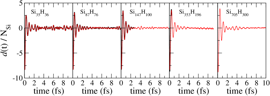
Figure 4: The dipole-dipole correlation function calculated using the TDsBSE approach with orthogonalization (red curves) compared with a direct time-dependent BSE approach (black curves). Note that the direct (i.e., non-stochastic) BSE approach is so expensive due to the full-exchange operation that it was not done for the largest NCs and was only followed for short times for intermediate size NCs.

In Fig. 4 we compare the dipole-dipole correlation function computed from the TDsBSE with $n_{\zeta}=1$ to the direct TDBSE approach for silicon nanocrystals of varying sizes (Si${}_{35}\mbox{H}_{36}$, Si${}_{87}\mbox{H}_{76}$, Si${}_{147}\mbox{H}_{100}$, Si${}_{353}\mbox{H}_{196}$, and Si${}_{705}\mbox{H}_{300}$). The purpose is to demonstrates the power of the TDsBSE approach with orthogonalization. Therefore, for simplicity $W\left({\bf r},{\bf r}^{\prime},0\right)$ is replaced by $\epsilon^{-1}v_{C}\left(\left|{\bf r}-{\bf r}^{\prime}\right|\right)$ with $\epsilon=5$ for all system sizes. Clearly, even when $n_{\zeta}=1$, the TDsBSE is in perfect agreement with the direct TDBSE approach. The cubic scaling of the later limits the application to small NCs or to short times.

In Fig. 5 we plot the TDsBSE absorption cross section ($\sigma\left(\omega\right)=\frac{e^{2}}{\epsilon_{0}c}\omega\int d{\bf r}d{\bf r}^{\prime}\,z\,{\bf\tilde{\chi}\left({\bf r},{\bf r}^{\prime},\omega\right)}\,z^{\prime}$) compared to the absorption cross section computed by ignoring the electron-hole interactions for a wide range of energies. It is practically impossible to obtain the absorption cross section over this wide energy range by a direct diagonalization of the symplectic eigenvalue equation (cf., Eq. (1)). Thus, so far the BSE has been applied to relatively small nanocrystals or by converging only the low lying excitonic transitions, even within the crude approximation where $W\left({\bf r},{\bf r}^{\prime},0\right)$ is replaced by $\epsilon^{-1}v_{C}\left(\left|{\bf r}-{\bf r}^{\prime}\right|\right)$. As far as we know the results shown in Fig. 5 are the first to report a converged BS calculations for NCs of experimentally relevant sizes. We used a constant $\epsilon$ in each run, with values of $5$, $6.2$, $7$, $8.2$, and $8.8$ taken from Ref. Wang and Zunger, 1994b for the silicon NCs (in ascending order) and $4.5$, $5$, $5.2$ and $5.4$ for the CdSe NCs taken from Ref. Wang and Zunger, 1996. The inclusion of a more accurate description of the screening as proposed in detailed in Appendix A is left open for future study.

For both types of NCs there is a shift of the onset of absorption to lower energies with increasing NC size due to the quantum confinement effect. The absorption cross section of the smallest NCs is characterized by detailed features, which are broadened and eventually washed out as the NC size increases. For silicon NCs, the semi-empirical pseudopotential model over-emphasizes the lowest excitonic transition in comparison to the plasmonic resonance observed at $\sim 10{\rm eV}$ using TDDFT.Chelikowsky, Kronik, and Vasiliev (2003); Tiago and Chelikowsky (2006); Ramos et al. (2008); Gao et al. (2015) It also misses the split of the lowest excitonic peak observed experimentally for bulk silicon and reproduced by the BSE approach,Rohlfing and Louie (2000); Sottile et al. (2007); Ramos et al. (2008); Rocca et al. (2012) but not by the current model ignoring electron-hole correlations.Wang and Zunger (1994b) The fact that the current calculation does not capture this split could be a consequence of the approximation used to model the screening.

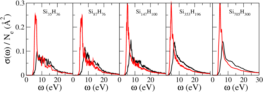
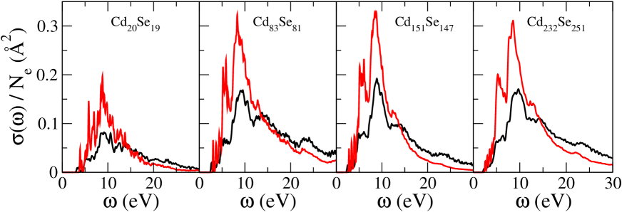
Figure 5: Upper panels: The absorption cross section for silicon NCs computed by Fourier transforming the TDsBSE dipole-dipole correlation function (black curves) and the corresponding absorption cross section computed for $\hat{h}_{qp}$, i.e., by ignoring electron-hole interactions.

The results for silicon NCs seem to imply that the inclusion of electron-hole interactions leads to a blue shift in the absorption cross section (black curve is shifted to higher energies compared to the red curve). Since silicon is an indirect band gap material, the onset of absorption is not a good measure of the strength of the electron-hole interactions. Indeed, when the approach is applied to CdSe NCs (lower panels of Fig. 5) the inclusion of electron-hole interaction clearly shifts the onset of absorption to lower energies.

IV Conclusions

We have developed a real-time stochastic approach to describe electron-hole excitations in extended finite systems based on the BSE. Following the logic connecting TDHF and CIS, we showed that a solution to a Schrödinger-like time-dependent equation for the quasiparticle orbitals with an effective Hamiltonian containing both direct and screened exchange terms is equivalent to the symplectic eigenvalue representation of the BSE. A direct solution of the TDBSE leads to at least cubic scaling with the system size due to the need to compute all occupied quasiparticle orbitals and the complexity of applying the screened exchange term to preform the time propagation. The lower bound is similar to the scaling of the TDHF method and thus, limits the application of the TDBSE approach to relatively small systems. To overcome this bottleneck, we developed a stochastic approach inspired by our previous work on stochastic GW Neuhauser et al. (2014) (sGW) and stochastic TDDFT,Gao et al. (2015) in which the occupied quasiparticle orbitals were replaced with stochastic orbitals. The latter were then used to obtain both the RPA screening using the approach developed for the screening in sGW and the exchange potential by extending the approach used todescribe the Hartree term in TDsDFT. Both the RPA screening the application of the exchange potential scale nearly linearly with system size (as opposed to quadratic scaling for example for the exchange potential). The number of stochastic orbitals required to converge the calculation scales with system size and thus, the overall scaling of the TDsBSE approach is quadratic (excluding the cubic contribution from the orthogonalization of the stochastic orbitals, which for the system sizes studied here is a negligible step).

We have applied the TDsBSE approach to study optical excitations in a wide range of energies (up to $30$ eV) in silicon and CdSe nanocrystals with sizes up to $\approx 3000$ electrons ($\approx 3$ nm diameter) and compared the results with the quasiparticle excitation spectrum obtained within the semi-empirical pseudopotential approach. For both systems, we find that including electron-hole correlations broadens the spectral features and shifts the oscillator strength to higher energies due to amplification of a plasmon resonance near $10$ eV. For silicon we find a surprising result where the onset optical excitations seem to shift to higher energies compared to the quasiparticle excitations. This is a result of two factors. First, silicon is an indirect band gap material and th the onset of optically allowed transitions is above the the lowest excitonic state. Second, the inclusion of electron-hole interactions via the BSE leads to an amplification of a plasmon resonance at $\approx 10$ eV shifting the oscillator strength to higher energies at the expense of the lower frequency absorption. These combined effects lead to an apparent shift of the absorption onset to higher energies when electron-hole interactions are included. This is not the case for CdSe, where the onset of optical excitation is below the onset of the quasiparticle excitation, as expect for a direct band-gap material.

The TDsBSE provides a platform to obtain optical excitations in extended systems covering a wide energy range. To overcome the divergent behavior at long times, it is necessary to increase the number of stochastic orbitals as the size of the system increases. We are working in improvements of this flaw and if solved, an even faster, linear scaling BS approach will emerge. This and other improvements as well as more general applications will be presented in a future work.

Appendix A: RPA screened exchange for TDsBSE

The above approach assumes that $W\left({\bf r},{\bf r}^{\prime},0\right)=v_{C}\left(\left|{\bf r}-{\bf r}^{\prime}\right|\right)+\delta W_{RPA}\left(\mathbf{r},\mathbf{r}^{\prime},0\right)$ is approximated by $\epsilon^{-1}v_{C}\left(\left|{\bf r}-{\bf r}^{\prime}\right|\right)$. In typical BS applications, one uses the RPA screening to describe $W\left({\bf r},{\bf r}^{\prime},0\right)=v_{C}\left(\left|\mathbf{r}-\mathbf{r}^{\prime}\right|\right)+\delta W\left(\mathbf{r},\mathbf{r}^{\prime},0\right)$. The stochastic formalism, however, furnishes a potentially viable approach to overcome the assumption made to obtain $W\left({\bf r},{\bf r}^{\prime},0\right)$ in this work. In the linear response limit, $\delta W_{RPA}\left(\mathbf{r},\mathbf{r}^{\prime},0\right)$ can be written as:

$$\delta W_{RPA}\left(\mathbf{r},\mathbf{r}^{\prime},0\right) =\iint d\mathbf{r}^{\prime\prime}d\mathbf{r}^{\prime\prime\prime}v_{C}\left(\left|{\bf r}-\mathbf{r}^{\prime\prime}\right|\right)$$

$$\tilde{\chi}_{RPA}\left({\bf\mathbf{r}}^{\prime\prime},{\bf r}^{\prime\prime\prime},0\right)\times$$

$$\left(v_{C}\left(\left|{\bf r}^{\prime\prime\prime}-{\bf r}^{\prime}\right|\right)+f_{XC}\mbox{$\left(\mathbf{r}^{\prime\prime\prime}\right)$}\delta\mbox{$\left({\bf r}^{\prime\prime\prime}-{\bf r}^{\prime}\right)$}\right),$$ (22)

and we are concerned with the application of $\hat{k}_{\epsilon X}^{\gamma}\left(t\right)$ on $\psi\left(\mathbf{r},t\right)$, or more accurately, the portion that depends on the screening:

$$\delta\hat{k}_{\epsilon X}^{\gamma}\left(t\right)=\eta_{x}^{\gamma}\left(\mathbf{r},t\right)\mbox{$\int$d{r}}^{\prime}\delta W_{RPA}\left({\bf r},{\bf r}^{\prime},0\right)\eta_{x}^{\gamma}\left(\mathbf{r}^{\prime},t\right)^{*}\psi\left(\mathbf{r}^{\prime},t\right).$$ (23)

We first insert Eq. (8) into Eq. (23):

$$\delta\hat{k}_{\epsilon X}^{\gamma}\left(t\right)\psi\left(\mathbf{r},t\right) =\eta_{x}^{\gamma}\left(\mathbf{r},t\right)\iint\mbox{$\int$d{r}}^{\prime}d\mathbf{r}^{\prime\prime}d\mathbf{r}^{\prime\prime\prime}$$

$$v_{C}\left(\left|{\bf r}-\mathbf{r}^{\prime\prime}\right|\right) \tilde{\chi}_{RPA}\left({\bf\mathbf{r}}^{\prime\prime},{\bf r}^{\prime\prime\prime},0\right)\left(v_{C}\left(\left|{\bf r}^{\prime\prime\prime}-{\bf r}^{\prime}\right|\right)\right.$$

$$+ \left.f_{XC}\mbox{$\left(\mathbf{r}^{\prime\prime\prime}\right)$}\delta\mbox{$\left({\bf r}^{\prime\prime\prime}-{\bf r}^{\prime}\right)$}\right)\eta_{x}^{\gamma}\left(\mathbf{r}^{\prime},t\right)^{*}\psi\left(\mathbf{r}^{\prime},t\right).$$ (24)

Define a perturbation potential

$$v^{\gamma}\left(\mathbf{r},t\right) =\int d\mathbf{r}^{\prime}\left(v_{C}\left(\left|{\bf r}^{\prime\prime\prime}-{\bf r}^{\prime}\right|\right)\right.$$

$$+ \left.f_{XC}\mbox{$\left(\mathbf{r}^{\prime\prime\prime}\right)$}\delta\mbox{$\left({\bf r}^{\prime\prime\prime}-{\bf r}^{\prime}\right)$}\right)\eta_{x}^{\gamma}\left(\mathbf{r}^{\prime},t\right)^{*}\psi\left(\mathbf{r}^{\prime},t\right)$$ (25)

and rewrite Eq. (24) as:

$$\delta\hat{k}_{\epsilon X}^{\gamma}\left(t\right)\psi\left(\mathbf{r},t\right) =\eta_{x}^{\gamma}\left(\mathbf{r},t\right)\iint d\mathbf{r}^{\prime}d\mathbf{r}^{\prime\prime}$$

$$v_{C}\left(\left|{\bf r}-\mathbf{r}^{\prime}\right|\right) \tilde{\chi}_{RPA}\left({\bf\mathbf{r}}^{\prime},{\bf r}^{\prime\prime},0\right)v^{\gamma}\left(\mathbf{r}^{\prime\prime},t\right).$$ (26)

The action of $\tilde{\chi}_{RPA}\left({\bf\mathbf{r}}^{\prime},{\bf r}^{\prime\prime},0\right)$ on $v^{\gamma}\left(\mathbf{r}^{\prime\prime},t\right)$ is manageable by using a stochastic TDDFT algorithm:Gao et al. (2015)

1. Take$N_{RPA}$ projected stochastic orbitals from the $N_{\zeta}$ generated above. If $N_{RPA}>N_{\zeta}$ generate additional projected stochastic orbitals following the prescription given in 1 and 2 above. This needs to be done just once, i.e., at the beginning of the calculation, generate enough projected stochastic orbitals to be used throughout the calculation.

2. Apply a perturbation at $\tau=0$: $\chi_{j}^{\gamma^{\prime}}\left({\bf r},\tau=0\right)=e^{-i\gamma^{\prime}v^{\gamma}\left({\bf r},t\right)/\hbar}\xi_{j}\left({\bf r}\right)$, where $\gamma^{\prime}$ is the strength of the RPA perturbation. Note that at each time $t$ used for solving the TDsBSE, one has to apply a different perturbation $v^{\gamma}\left({\bf r},t\right)$ at $\tau=0$, which is used to indicate the time for the RPA propagation.

3. Propagate the orbitals using the adiabatic stochastic time-dependent equations:

   $$i\hbar\frac{\partial\chi_{j}^{\gamma^{\prime}}\left({\bf r},\tau\right)}{\partial\tau} =\hat{h}_{RPA}^{\gamma^{\prime}}\left(\tau\right)\chi_{j}^{\gamma^{\prime}}\left({\bf r},\tau\right),$$ (27)

   Here, one can take $\hat{h}_{RPA}^{\gamma^{\prime}}\left(\tau\right)=\hat{h}_{qp}$ or $\hat{h}_{RPA}^{\gamma^{\prime}}\left(\tau\right)=\hat{h}_{qp}+v_{HXC}\left[n_{RPA}^{\gamma^{\prime}}\left(\tau\right)\right]\left(\mathbf{r}\right)-v_{HXC}\left[n_{RPA}^{0}\left(\tau\right)\right]\left(\mathbf{r}\right)$. For the latter case, $v_{HXC}\left[n\right]\left(\mathbf{r}\right)=\int d\mathbf{r}^{\prime}\frac{n\left(\mathbf{r}^{\prime}\right)}{\left|\mathbf{r}-\mathbf{r}^{\prime}\right|}+v_{XC}\left(n\left(\mathbf{r}\right)\right)$ and $v_{XC}\left(n\left(\mathbf{r}\right)\right)$ is the local density (or semi-local) approximation for the exchange correlation potential. The density is obtained as an average over the RPA stochastic orbital densities:

   $$n_{RPA}^{\gamma^{\prime}}\left({\bf{\bf r}},\tau\right) =\frac{2}{N_{RPA}}\sum_{j=1}^{N_{RPA}}\left|\chi_{j}^{\gamma^{\prime}}\left({\bf r},\tau\right)\right|^{2}$$ (28)

4. Generate $\Delta n_{RPA}\left({\bf r},\tau\right)=\frac{1}{\gamma^{\prime}}\left(n_{RPA}^{\gamma^{\prime}}\left({\bf r},\tau\right)-n_{RPA}^{0}\left({\bf r},\tau\right)\right)$ and its half Fourier transformed quantity $\Delta\tilde{n}_{RPA}\left(\mathbf{r},0\right)$ at $\omega=0$.

5. Obtain the action of $\delta\hat{k}_{\epsilon X}^{\gamma}\left(t\right)\psi\left(\mathbf{r},t\right)=\eta_{x}^{\gamma}\left(\mathbf{r},t\right)\iint d\mathbf{r}^{\prime}d\mathbf{r}^{\prime\prime}v_{C}\left(\left|{\bf r}-\mathbf{r}^{\prime}\right|\right)\tilde{\chi}_{RPA}\left({\bf\mathbf{r}}^{\prime},{\bf r}^{\prime\prime},0\right)v^{\gamma}\left(\mathbf{r}^{\prime\prime},t\right)$ from $\delta\hat{k}_{\epsilon X}\left(t\right)\psi\left(\mathbf{r},t\right)=\eta_{x}^{\gamma}\left(\mathbf{r},t\right)\iint d\mathbf{r}^{\prime}d\mathbf{r}^{\prime\prime}v_{C}\left(\left|{\bf r}-\mathbf{r}^{\prime}\right|\right)\Delta\tilde{n}_{RPA}\left({\bf r}^{\prime},0\right)$.

Step 1-5 need to be repeated at each time step $\Delta t$ of the TDsBSE propagation.

Appendix B: Ehrenfest theorem

Ehrenfest theorem asserts that a correct propagation must preserve the relation

$$\left\langle\dot{\mathbf{q}}\left(t\right)\right\rangle=i\left\langle\left[\hat{h}_{BS},\hat{\mathbf{q}}\right]\right\rangle$$ (29)

For a TDBSE this relation is given by

$$i\left\langle\left[\hat{h}_{BS},\hat{\mathbf{q}}\right]\right\rangle=\frac{\left\langle\mathbf{p}\left(t\right)\right\rangle}{m}+i\left\langle\left[\hat{k}_{\epsilon X}^{\gamma}\left(t\right)-\hat{k}_{\epsilon X}^{0}\left(t\right),\hat{\mathbf{q}}\right]\right\rangle$$ (30)

where $\hat{k}_{\epsilon X}^{\gamma}\left(t\right)\psi\left(\mathbf{r}\right)=-\frac{1}{2}\int d\mathbf{r}^{\prime}\rho^{\gamma}\left(\mathbf{r},{\bf r}^{\prime},t\right)W^{RPA}\left({\bf r},{\bf r}^{\prime},0\right)\psi\left(\mathbf{r}^{\prime}\right)$. To satisfy the Ehrenfest theorem $\left\langle\left[\hat{k}_{\epsilon X}^{\gamma}\left(t\right)-\hat{k}_{\epsilon X}^{0}\left(t\right),\hat{\mathbf{q}}\right]\right\rangle$ should vanish. The commutator of the exchange operator is given by:

$$i\left\langle\left[\hat{k}_{\epsilon X}^{\gamma}\left(t\right),\hat{\mathbf{q}}\right]\right\rangle = -\frac{i}{2}\iint d^{3}rd^{3}r^{\prime}\left|\rho^{\gamma}\left(\mathbf{r},{\bf r}^{\prime},t\right)\right|^{2}$$ (31)

$$\times W^{RPA}\left({\bf r},{\bf r}^{\prime},0\right)\left(\mathbf{r}-\mathbf{r}^{\prime}\right).$$

In the above, the commuter vanishes for the $\hat{k}_{\epsilon X}^{\gamma}\left(t\right)$ term due to symmetry, but there is no a-priori reason why the $\hat{k}_{\epsilon X}^{0}\left(t\right)$ term should vanish. However, as illustrated numerically in Fig. 2, the contribution of this non-vanishing term is rather small even on timescales much larger than the typical frequency in the system.

References

- Coe, Woo, and Moungi Bawendi (2002) S. Coe, W.-K. Woo, and V. B. Moungi Bawendi, Nature 420, 800 (2002).
- Tessler et al. (2002) N. Tessler, V. Medvedev, M. Kazes, S. H. Kan, and U. Banin, Science 295, 1506 (2002).
- Gur et al. (2005) I. Gur, N. A. Fromer, M. L. Geier, and A. P. Alivisatos, Science 310, 462 (2005).
- Talapin and Murray (2005) D. V. Talapin and C. B. Murray, Science 310, 86 (2005).
- Runge and Gross (1984) E. Runge and E. K. U. Gross, Phys. Rev. Lett. 52, 997 (1984).
- van Leeuwen (2001) R. van Leeuwen, Inter. J. Moder. Phys. B 15, 1969 (2001).
- Onida, Reining, and Rubio (2002) G. Onida, L. Reining, and A. Rubio, Rev. Mod. Phys. 74, 601 (2002).
- Maitra et al. (2002) N. T. Maitra, K. Burke, H. Appel, and E. K. U. Gross, “Ten topical questions in time dependent density functional theory,” in Reviews in Modern Quantum Chemistry: A celebration of the contributions of R. G. Parr, Vol. II, edited by K. D. Sen (World-Scientific, Singapore, 2002) p. 1186.
- Marques and Gross (2004) M. Marques and E. Gross, Annu. Rev. Phys. Chem. 55, 427 (2004).
- Burke, Werschnik, and Gross (2005) K. Burke, J. Werschnik, and E. K. U. Gross, J. Chem. Phys. 123, 062206 (2005).
- Botti et al. (2007) S. Botti, A. Schindlmayr, R. Del Sole, and L. Reining, Rep. Prog. Phys. 70, 357 (2007).
- Jacquemin et al. (2009) D. Jacquemin, E. A. Perpete, I. Ciofini, and C. Adamo, Acc. Chem. Res. 42, 326 (2009).
- Casida (2009) M. E. Casida, J. Mol. Struct. 914, 3 (2009).
- Adamo and Jacquemin (2013) C. Adamo and D. Jacquemin, Chem. Soc. Rev. 42, 845 (2013).
- Stratmann, Scuseria, and Frisch (1998) R. E. Stratmann, G. E. Scuseria, and M. J. Frisch, J. Chem. Phys. 109, 8218 (1998).
- Yabana and Bertsch (1996) K. Yabana and G. F. Bertsch, Phys. Rev. B 54, 4484 (1996).
- Bertsch et al. (2000) G. F. Bertsch, J. I. Iwata, A. Rubio, and K. Yabana, Phys. Rev. B 62, 7998 (2000).
- Baer and Neuhauser (2004) R. Baer and D. Neuhauser, J. Chem. Phys. 121, 9803 (2004).
- Bauernschmitt and Ahlrichs (1996) R. Bauernschmitt and R. Ahlrichs, Chem. Phys. Lett. 256, 454 (1996).
- Bauernschmitt et al. (1998) R. Bauernschmitt, R. Ahlrichs, F. H. Hennrich, and M. M. Kappes, J. Am. Chem. Soc. 120, 5052 (1998).
- Fabian (2001) J. Fabian, Theor. Chem. Acc. 106, 199 (2001).
- Vasiliev, Ogut, and Chelikowsky (2002) I. Vasiliev, S. Ogut, and J. R. Chelikowsky, Phys. Rev. B 65, 115416 (2002).
- Shao, Head-Gordon, and Krylov (2003) Y. H. Shao, M. Head-Gordon, and A. I. Krylov, J. Chem. Phys. 118, 4807 (2003).
- Troparevsky, Kronik, and Chelikowsky (2003) M. C. Troparevsky, L. Kronik, and J. R. Chelikowsky, J. Chem. Phys. 119, 2284 (2003).
- Maitra (2005) N. T. Maitra, J. Chem. Phys. 122, 234104 (2005).
- Andzelm et al. (2007) J. Andzelm, A. M. Rawlett, J. A. Orlicki, and J. F. Snyder, J. Chem. Theory Comput. 3, 870 (2007).
- Govind et al. (2009) N. Govind, M. Valiev, L. Jensen, and K. Kowalski, J. Phys. Chem. A 113, 6041 (2009).
- Peach et al. (2009) M. J. G. Peach, C. R. Le Sueur, K. Ruud, M. Guillaume, and D. J. Tozer, Phys. Chem. Chem. Phys. 11, 4465 (2009).
- Kuritz et al. (2011) N. Kuritz, T. Stein, R. Baer, and L. Kronik, J. Chem. Theory Comput. 7, 2408 (2011).
- Peach, Williamson, and Tozer (2011) M. J. G. Peach, M. J. Williamson, and D. J. Tozer, J. Chem. Theory Comput. 7, 3578 (2011).
- Srebro et al. (2011) M. Srebro, N. Govind, W. A. de Jong, and J. Autschbach, J. Phys. Chem. A 115, 10930 (2011).
- Richard and Herbert (2011) R. M. Richard and J. M. Herbert, J. Chem. Theory Comput. 7, 1296 (2011).
- Chantzis et al. (2013) A. Chantzis, A. D. Laurent, C. Adamo, and D. Jacquemin, J. Chem. Theory Comput. 9, 4517 (2013).
- Bauernschmitt et al. (1997) R. Bauernschmitt, M. Haser, O. Treutler, and R. Ahlrichs, Chem. Phys. Lett. 264, 573 (1997).
- Chelikowsky, Kronik, and Vasiliev (2003) J. R. Chelikowsky, L. Kronik, and I. Vasiliev, J. Phys. Condes. Matrer 15, R1517 (2003).
- Gavnholt et al. (2009) J. Gavnholt, A. Rubio, T. Olsen, K. S. Thygesen, and J. Schiotz, Phys. Rev. B 79, 195405 (2009).
- Hirata and Head-Gordon (1999a) S. Hirata and M. Head-Gordon, Chem. Phys. Lett. 302, 375 (1999a).
- Hirata, Lee, and Head-Gordon (1999) S. Hirata, T. J. Lee, and M. Head-Gordon, J. Chem. Phys. 111, 8904 (1999).
- Jacquemin et al. (2008) D. Jacquemin, E. A. Perpete, G. E. Scuseria, I. Ciofini, and C. Adamo, J. Chem. Theory Comput. 4, 123 (2008).
- Stein, Kronik, and Baer (2009a) T. Stein, L. Kronik, and R. Baer, J. Chem. Phys. 131, 244119 (2009a).
- Stein, Kronik, and Baer (2009b) T. Stein, L. Kronik, and R. Baer, J. Am. Chem. Soc. 131, 2818 (2009b).
- Phillips et al. (2011) H. Phillips, S. Zheng, A. Hyla, R. Laine, T. Goodson, E. Geva, and B. D. Dunietz, J. Phys. Chem. A 116, 1137 (2011).
- Ou et al. (2014) Q. Ou, S. Fatehi, E. Alguire, Y. Shao, and J. E. Subotnik, J. Chem. Phys. 141, 024114 (2014).
- Parac and Grimme (2003) M. Parac and S. Grimme, Chem. Phys. 292, 11 (2003).
- Grimme and Parac (2003) S. Grimme and M. Parac, Chem. Phys. Chem. 4, 292 (2003).
- Dreuw and Head-Gordon (2004) A. Dreuw and M. Head-Gordon, J. Am. Chem. Soc. 126, 4007 (2004).
- Maitra et al. (2004) N. T. Maitra, F. Zhang, R. J. Cave, and K. Burke, J. Chem. Phys. 120, 5932 (2004).
- Hieringer and Görling (2006) W. Hieringer and A. Görling, Chem. Phys. Lett. 419, 557 (2006).
- Levine et al. (2006) B. G. Levine, C. Ko, J. Quenneville, and T. J. Martinez, Mol. Phys. 104, 1039 (2006).
- Lopata et al. (2011) K. Lopata, R. Reslan, M. Kowaska, D. Neuhauser, N. Govind, and K. Kowalski, J. Chem. Theory Comput. 7, 3686 (2011).
- Kowalczyk, Yost, and Van Voorhis (2011) T. Kowalczyk, S. R. Yost, and T. Van Voorhis, J. Chem. Phys. 134, 054128 (2011).
- Isborn et al. (2013) C. M. Isborn, B. D. Mar, B. F. Curchod, I. Tavernelli, and T. J. Martínez, J. Phys. Chem. B 117, 12189 (2013).
- Albrecht et al. (1998) S. Albrecht, L. Reining, R. Del Sole, and G. Onida, Phys. Rev. Lett. 80, 4510 (1998).
- Rohlfing and Louie (2000) M. Rohlfing and S. G. Louie, Phys. Rev. B 62, 4927 (2000).
- Sottile et al. (2007) F. Sottile, M. Marsili, V. Olevano, and L. Reining, Phys. Rev. B 76, 161103 (2007).
- Ramos et al. (2008) L. Ramos, J. Paier, G. Kresse, and F. Bechstedt, Phys. Rev. B 78, 195423 (2008).
- Rocca et al. (2012) D. Rocca, Y. Ping, R. Gebauer, and G. Galli, Phys. Rev. B 85, 045116 (2012).
- Hedin (1965) L. Hedin, Phys. Rev. 139, A796 (1965).
- Salpeter and Bethe (1951) E. E. Salpeter and H. A. Bethe, Phys. Rev. 84, 1232 (1951).
- Hybertsen and Louie (1985) M. S. Hybertsen and S. G. Louie, Phys. Rev. Lett. 55, 1418 (1985).
- Hybertsen and Louie (1986) M. S. Hybertsen and S. G. Louie, Phys. Rev. B 34, 5390 (1986).
- Steinbeck et al. (1999) L. Steinbeck, A. Rubio, L. Reining, M. Torrent, I. White, and R. Godby, Comput. Phys. Commun. 125, 05 (1999).
- Rieger et al. (1999) M. M. Rieger, L. Steinbeck, I. White, H. Rojas, and R. Godby, Comput. Phys. Commun. 117, 211 (1999).
- Rinke et al. (2005) P. Rinke, A. Qteish, J. Neugebauer, C. Freysoldt, and M. Scheffler, New J. Phys. 7, (2005).
- Neaton, Hybertsen, and Louie (2006) J. B. Neaton, M. S. Hybertsen, and S. G. Louie, Phys. Rev. Lett. 97, 216405 (2006).
- Tiago and Chelikowsky (2006) M. L. Tiago and J. R. Chelikowsky, Phys. Rev. B 73, 205334 (2006).
- Friedrich and Schindlmayr (2006) C. Friedrich and A. Schindlmayr, NIC Series 31, 335 (2006).
- Gruning, Marini, and Rubio (2006) M. Gruning, A. Marini, and A. Rubio, J. Chem. Phys. 124, 154108 (2006).
- Shishkin and Kresse (2007) M. Shishkin and G. Kresse, Phys. Rev. B 75, 235102 (2007).
- Huang and Carter (2008) P. Huang and E. A. Carter, Annu. Rev. Phys. Chem. 59, 261 (2008).
- Rostgaard, Jacobsen, and Thygesen (2010) C. Rostgaard, K. W. Jacobsen, and K. S. Thygesen, Phys. Rev. B 81, 085103 (2010).
- Tamblyn et al. (2011) I. Tamblyn, P. Darancet, S. Y. Quek, S. A. Bonev, and J. B. Neaton, Phys. Rev. B 84, 201402 (2011).
- Liao and Carter (2011) P. Liao and E. A. Carter, Phys. Chem. Chem. Phys. 13, 15189 (2011).
- Refaely-Abramson, Baer, and Kronik (2011) S. Refaely-Abramson, R. Baer, and L. Kronik, Phys. Rev. B 84, 075144 (2011).
- Marom et al. (2012) N. Marom, F. Caruso, X. Ren, O. T. Hofmann, T. Körzdörfer, J. R. Chelikowsky, A. Rubio, M. Scheffler, and P. Rinke, Phys. Rev. B 86, 245127 (2012).
- Isseroff and Carter (2012) L. Y. Isseroff and E. A. Carter, Phys. Rev. B 85, 235142 (2012).
- Refaely-Abramson et al. (2012) S. Refaely-Abramson, S. Sharifzadeh, N. Govind, J. Autschbach, J. B. Neaton, R. Baer, and L. Kronik, Phys. Rev. Lett. 109, 226405 (2012).
- Kronik et al. (2012) L. Kronik, T. Stein, S. Refaely-Abramson, and R. Baer, J. Chem. Theory Comput. 8, 1515 (2012).
- Benedict, Shirley, and Bohn (1998) L. X. Benedict, E. L. Shirley, and R. B. Bohn, Phys. Rev. Lett. 80, 4514 (1998).
- Benedict et al. (2003) L. X. Benedict, A. Puzder, A. J. Williamson, J. C. Grossman, G. Galli, J. E. Klepeis, J.-Y. Raty, and O. Pankratov, Phys. Rev. B 68, 085310 (2003).
- Spataru et al. (2004) C. D. Spataru, S. Ismail-Beigi, L. X. Benedict, and S. G. Louie, Phys. Rev. Lett. 92, 077402 (2004).
- Sai et al. (2008) N. Sai, M. L. Tiago, J. R. Chelikowsky, and F. A. Reboredo, Phys. Rev. B 77, 161306 (2008).
- Fuchs et al. (2008) F. Fuchs, C. Rödl, A. Schleife, and F. Bechstedt, Phys. Rev. B 78, 085103 (2008).
- Palummo et al. (2009) M. Palummo, C. Hogan, F. Sottile, P. Bagala, and A. Rubio, J. Chem. Phys. 131, 084102 (2009).
- Schimka et al. (2010) L. Schimka, J. Harl, A. Stroppa, A. Gruneis, M. Marsman, F. Mittendorfer, and G. Kresse, Nat. Mater. 9, 741 (2010).
- Rocca, Lu, and Galli (2010) D. Rocca, D. Lu, and G. Galli, J. Chem. Phys. 133, 164109 (2010).
- Blase and Attaccalite (2011) X. Blase and C. Attaccalite, Appl. Phys. Lett. 99, 171909 (2011).
- Faber et al. (2012) C. Faber, I. Duchemin, T. Deutsch, C. Attaccalite, V. Olevano, and X. Blase, J. Mater. Sci. 47, 7472 (2012).
- Faber et al. (2014) C. Faber, P. Boulanger, C. Attaccalite, I. Duchemin, and X. Blase, Philos. Trans. A Math. Phys. Eng. Sci. 372, 20130271 (2014).
- Walker et al. (2006) B. Walker, A. M. Saitta, R. Gebauer, and S. Baroni, Phys. Rev. Lett. 96, 113001 (2006).
- Rocca et al. (2008) D. Rocca, R. Gebauer, Y. Saad, and S. Baroni, J. Chem. Phys. 128, 154105 (2008).
- Wilson, Gygi, and Galli (2008) H. F. Wilson, F. Gygi, and G. Galli, Phys. Rev. B 78, 113303 (2008).
- Baroni et al. (2001) S. Baroni, S. de Gironcoli, A. Dal Corso, and P. Giannozzi, Rev. Mod. Phys. 73, 515 (2001).
- Baer, Neuhauser, and Rabani (2013) R. Baer, D. Neuhauser, and E. Rabani, Phys. Rev. Lett. 111, 106402 (2013).
- Neuhauser, Baer, and Rabani (2014) D. Neuhauser, R. Baer, and E. Rabani, J. Chem. Phys. 141, 041102 (2014).
- Neuhauser, Rabani, and Baer (2013a) D. Neuhauser, E. Rabani, and R. Baer, J. Chem. Theory Comput. 9, 24 (2013a).
- Ge et al. (2013) Q. Ge, Y. Gao, R. Baer, E. Rabani, and D. Neuhauser, J. Phys. Chem. Lett. 5, 185 (2013).
- Neuhauser, Rabani, and Baer (2013b) D. Neuhauser, E. Rabani, and R. Baer, J. Phys. Chem. Lett. 4, 1172 (2013b).
- Baer and Rabani (2012) R. Baer and E. Rabani, Nano Lett. 12, 2123 (2012).
- Neuhauser et al. (2014) D. Neuhauser, Y. Gao, C. Arntsen, C. Karshenas, E. Rabani, and R. Baer, Phys. Rev. Lett. 113, 076402 (2014).
- Gao et al. (2015) Y. Gao, D. Neuhauser, R. Baer, and E. Rabani, J. Chem. Phys. 142, 034106 (2015).
- Casida (1995) M. E. Casida, Recent advances in density functional methods 1, 155 (1995).
- Casida (1996) M. E. Casida, “Time-dependent density functional response theory of molecular systems: theory, computational methods, and functionals,” in Recent Developments and Applications in Density Functional Theory, edited by J. M. Seminario (Elsevier, Amsterdam, 1996) pp. 391–439.
- Furche (2001) F. Furche, Phys. Rev. B 64, 195120 (2001).
- Dyson (1953) F. J. Dyson, Phys. Rev. 90, 994 (1953).
- Taylor (1954) J. Taylor, Phys. Rev. 95, 1313 (1954).
- Hirata and Head-Gordon (1999b) S. Hirata and M. Head-Gordon, Chem. Phys. Lett. 314, 291 (1999b).
- Hirata, Head-Gordon, and Bartlett (1999) S. Hirata, M. Head-Gordon, and R. J. Bartlett, J. Chem. Phys. 111, 10774 (1999).
- Baer and Neuhauser (2005) R. Baer and D. Neuhauser, Phys. Rev. Lett. 94, 043002 (2005).
- Brothers et al. (2008) E. N. Brothers, A. F. Izmaylov, J. O. Normand, V. Barone, and G. E. Scuseria, J. Chem. Phys. 129, 011102 (2008).
- Wang and Zunger (1994a) L. W. Wang and A. Zunger, J. Phys. Chem. 98, 2158 (1994a).
- Wang and Zunger (1995) L. W. Wang and A. Zunger, Phys. Rev. B 51, 17398 (1995).
- Wang and Zunger (1996) L. W. Wang and A. Zunger, Phys. Rev. B 53, 9579 (1996).
- Fu and Zunger (1997a) H. Fu and A. Zunger, Phys. Rev. B 55, 1642 (1997a).
- Williamson and Zunger (2000) A. J. Williamson and A. Zunger, Phys. Rev. B 61, 1978 (2000).
- Franceschetti and Zunger (2000a) A. Franceschetti and A. Zunger, Phys. Rev. B 62, 2614 (2000a).
- Zunger (2001) A. Zunger, Physica Status Solidi B-Basic Research 224, 727 (2001).
- Fu and Zunger (1997b) H. X. Fu and A. Zunger, Phys. Rev. B 56, 1496 (1997b).
- Rabani et al. (1999) E. Rabani, B. Hetenyi, B. J. Berne, and L. E. Brus, J. Chem. Phys. 110, 5355 (1999).
- Reboredo, Franceschetti, and Zunger (2000) F. A. Reboredo, A. Franceschetti, and A. Zunger, Phys. Rev. B 61, 13073 (2000).
- Franceschetti and Zunger (2000b) A. Franceschetti and A. Zunger, Phys. Rev. B 62, R16287 (2000b).
- Eshet, Grünwald, and Rabani (2013) H. Eshet, M. Grünwald, and E. Rabani, Nano Lett. 13, 5880 (2013).
- Wang and Zunger (1994b) L. W. Wang and A. Zunger, Phys. Rev. Lett. 73, 1039 (1994b).
- Zunger and Wang (1996) A. Zunger and L. W. Wang, Appl. Surf. Sci. 102, 350 (1996).
- Kosloff (1988) R. Kosloff, J. Phys. Chem. 92, 2087 (1988).