Electrocaloric effect in KH₂PO₄ family crystals

Abstract

The proton ordering model for the KH₂PO₄ type ferroelectrics is modified by taking into account the dependence of the effective dipole moments on the proton ordering parameter. Within the four-particle cluster approximation we calculate the crystal polarization and explore the electrocaloric effect. Smearing of the ferroelectric phase transition by a longitudinal electric field is described. A good agreement with experiment is obtained.

Key words: electrocaloric effect, KDP, cluster approximation, polarization

PACS: 77.84.Fa, 77.70.+a

Abstract

В моделi протонного впорядкування для кристалiв типу KH₂PO₄ враховано залежнiсть ефективних дипольних моментiв вiд параметра протонного впорядкування. В наближеннi чотиричастинкового кластера розраховано поляризацiю кристалiв та дослiджено електрокалоричний ефект у них. Описано розмивання сегнетоелектричного фазового переходу поздовжним електричним полем. Отримано добре узгодження з експериментальними даними.

Ключовi слова: електрокалоричний ефект, KDP, кластерне наближення, поляризацiя

1 Introduction

The electrocaloric (EC) effect is the change of temperature of a dielectric at an adiabatic change of the applied electric field. Research in this field is driven by a quest for materials that can be used for efficient, environment-friendly, and compact (on-chip) solid-state cooling devices.

The current state of the art on the electrocaloric effect research for ferroelectrics is well summarized in [2, 1]. At the moment, the largest effect is observed in perovskite ferroelectrics. Thus, in [3] in the PbZr_0.95Ti_0.05O₃ thin film with a thickness of 350 nm in a strong electric field (480 kV/cm) the obtained electrocaloric temperature change is $\Delta T=12$ K. Ab initio molecular dynamics calculations [4] predict $\Delta T\thickapprox 20$ K in LiNbO₃. In the hydrogen bonded ferroelectrics of the KH₂PO₄ (KDP) type, the electrocaloric effect was studied for relatively low fields only. Thus, it has been obtained that $\Delta T\thickapprox 0.04$ K at $E\thickapprox 4$ kV/cm [5], $\Delta T\thickapprox~{}1$ K at $E\thickapprox 12$ kV/cm [6], and $\Delta T\thickapprox 0.25$ K at $T_{\textrm{c}}$ and $E\thickapprox 1.2$ kV/cm [7].

Theoretical calculations of the electrocaloric effect in KDP have been made in [8] within the Slater model [9] and in the paraelectric phase only. It is also known that the Slater model gives incorrect results in the ferroelectric phase, and more complicated versions of the proton ordering model are required for an adequate description of these crystals. Thus, the effect of electric field on the physical characteristics of the KDP type crystals, such as polarization, dielectric permittivity, piezoelectric coefficients, elastic constants, has been described within the proton ordering model with the piezoelectric coupling to the shear strain $\varepsilon_{6}$ [10, 11, 12] and with proton tunneling [13] taken into account. However, these theories required, in particular, invoking two different values of the effective dipole moments for the paraelectric and ferroelectric phase [10, 12]. This made impossible a correct description of the system behavior in the fields high enough to smear out the first order phase transition. There is an inner logical contradiction in the model: while no physical characteristic of a crystal should exhibit any discontinuity in the fields above the critical one, there is no smooth transition between the values of model parameters, rigidly set to be different for the two phases.

In the present paper we suggest a way to remove this contradiction. Assuming that the difference between the dipole moments is caused by non-zero values of the order parameter, we modify the proton ordering model accordingly. The field dependences of polarization, smearing of the first order phase transition, and the electrocaloric effect are described.

2 Thermodynamic characteristics

We consider the KDP type ferroelectrics in the presence of an external electric field $E_{3}$ applied along the crystallographic axis c, inducing the strain $\varepsilon_{6}$ and polarization $P_{3}$. The total model Hamiltonian reads

$$\hat{H}=N\hat{H}_{0}+\hat{H}_{\textrm{s}}\,,$$ (1)

where $N$ is the total number of primitive cells. The ‘‘seed’’ energy $H_{0}$ corresponds to the sublattice of heavy ions and does not explicitly depend on the proton subsystem configuration. It is expressed in terms of the strain $\varepsilon_{6}$ and electric field $E_{3}$ and includes the elastic, piezoelectric, and dielectric contributions [11]

$$\hat{H}_{0}={v}\left(\frac{1}{2}c_{66}^{E0}\varepsilon_{6}^{2}-e_{36}^{0}E_{3}\varepsilon_{6}-\frac{1}{2}\chi_{33}^{\varepsilon 0}E_{3}^{2}\right),$$ (2)

where $v$ is the primitive cell volume; $c_{44}^{E0}$, $e_{36}^{0}$, ${\chi}_{33}^{\varepsilon 0}$ are the ‘‘seed’’ elastic constant, piezoelectric coefficient, and dielectric susceptibility, respectively.

The pseudospin part of the Hamiltonian reads

$$\hat{H}_{\textrm{s}}=\frac{1}{2}\sum\limits_{{qf},{q^{\prime}f^{\prime}}}J_{ff^{\prime}}(qq^{\prime})\frac{\sigma_{qf}}{2}\frac{\sigma_{q^{\prime}f^{\prime}}}{2}+\hat{H}_{\textrm{sh}}+\sum\limits_{qf}2\psi_{6}\varepsilon_{6}\frac{\sigma_{qf}}{2}-\sum\limits_{qf}\mu_{f}E_{3}\frac{\sigma_{qf}}{2}+\hat{H}_{E}\,.$$ (3)

Here, the first term describes the effective long-range interactions between protons, including also indirect lattice-mediated interactions [14, 15]; $\sigma_{qf}$ is the operator of the $z$-component of a pseudospin, corresponding to the proton on the $f$-th hydrogen bond ($f=1,\,2,\,3,\,4$) in the $q$-th cell. Its eigenvalues $\sigma_{qf}=\pm 1$ are assigned to two equilibrium positions of a proton on this bond.

In (3), $\hat{H}_{\textrm{sh}}$ is the Hamiltonian of short-range interactions between protons, which includes terms linear over the strain [11]

$$\hat{H}_{\textrm{sh}} = \sum\limits_{q}\bigg{\{}\left(\frac{\delta_{s}}{8}\varepsilon_{6}+\frac{\delta_{1}}{4}\varepsilon_{6}\right)(\sigma_{q1}+\sigma_{q2}+\sigma_{q3}+\sigma_{q4})$$ (4)

$$+\left(\frac{\delta_{s}}{8}\varepsilon_{6}-\frac{\delta_{1}}{4}\varepsilon_{6}\right)(\sigma_{q1}\sigma_{q2}\sigma_{q3}+\sigma_{q1}\sigma_{q2}\sigma_{q4}+\sigma_{q1}\sigma_{q3}\sigma_{q4}+\sigma_{q2}\sigma_{q3}\sigma_{q4})$$

$$+\frac{1}{4}(V+\delta_{a}\varepsilon_{6})(\sigma_{q1}\sigma_{q2}+\sigma_{q3}\sigma_{q4})+\frac{1}{4}(V-\delta_{a}\varepsilon_{6})(\sigma_{q2}\sigma_{q3}+\sigma_{q4}\sigma_{q1})$$

$$+\frac{U}{4}(\sigma_{q1}\sigma_{q3}+\sigma_{q2}\sigma_{q4})+\frac{\Phi}{16}\sigma_{q1}\sigma_{q2}\sigma_{q3}\sigma_{q4}\bigg{\}}.$$

Here,

$$V=-\frac{1}{2}w_{1}\,,\qquad U=\frac{1}{2}w_{1}-\varepsilon\,,\qquad\Phi=4\varepsilon-8w+2w_{1}\,,$$

and $\varepsilon$, $w$, $w_{1}$ are the energies of proton configurations.

The third term in (3) is a linear over the shear strain $\varepsilon_{6}$ field due to the piezoelectric coupling; $\psi_{6}$ is the deformational potential. The fourth term effectively describes the system interaction with the external electric field $E_{3}$. Here, $\mu_{f}$ is the effective dipole moment of the $f$-the hydrogen bond, and

$$\mu_{1}=\mu_{2}=\mu_{3}=\mu_{4}=\mu.$$

The fifth term in (3) is introduced in the present paper for the first time. It takes into account the assumed dependence of the effective dipole moment on the order parameter (pseudospin mean value)

$$\hat{H}_{E}=-\bigg{(}\frac{1}{N}\sum\limits_{q^{\prime}f^{\prime}}\frac{\sigma_{q^{\prime}f^{\prime}}}{2}\bigg{)}^{2}\mu^{\prime}E_{3}\sum\limits_{qf}\frac{\sigma_{qf}}{2}\,.$$ (5)

It is equivalent to a term proportional to $P_{3}^{3}E_{3}$ in a phenomenological thermodynamic potential. Note that the terms like $P_{3}^{2}E_{3}$ are not allowed because of the symmetry considerations, and we keep the Hamiltonian to be linear in the field $E_{3}$.

In view of the crystal structure of the KDP type ferroelectrics, the four-particle cluster approximation is most suitable for short-range interactions [15, 16]. Long-range interactions and the term $\hat{H}_{E}$ are taken into account in the mean field approximation. Thus,

$$\hat{H}_{E}\approx-12N\mu^{\prime}E_{3}\eta^{2}\sum\limits_{f=1}^{4}\frac{\sigma_{qf}}{2}+16N\mu^{\prime}E_{3}\eta^{3}.$$ (6)

Combining the fourth term in (3) and the first term in (6), we obtain the following term in the Hamiltonian $-(\mu+12\mu^{\prime}\eta^{2})E_{3}\sum_{qf}{\sigma_{qf}}/{2}$. Effectively, the term $12\mu^{\prime}\eta^{2}$ in $(\mu+12\mu^{\prime}\eta^{2})$ describes the jump of the dipole moment at the first order phase transition, its different values for the paraelectric and ferroelectric phase, and its smooth behavior in the fields above the critical one, when there is no jump of $\eta$. We can now use a single value of $\mu$ for both phases and remove the logical contradiction of the earlier theories, described in Introduction.

Proceeding with the standard calculations of the cluster approximation [10, 12, 16], we obtain the following expression for the proton ordering parameter

$$\eta=\langle\sigma_{q1}\rangle=\langle\sigma_{q2}\rangle=\langle\sigma_{q3}\rangle=\langle\sigma_{q4}\rangle=\frac{m}{D}\,,$$

where

$$m =\sinh(2z+\beta\delta_{s}\varepsilon_{6})+2b\sinh(z-\beta\delta_{1}\varepsilon_{6}),$$

$$D =\cosh(2z+\beta\delta_{s}\varepsilon_{6})+4b\cosh(z-\beta\delta_{1}\varepsilon_{6})+2a\cosh\beta\delta_{a}\varepsilon_{6}+d,$$

$$z =\frac{1}{2}\ln\frac{1+\eta}{1-\eta}+\beta\nu_{\textrm{c}}\eta-\beta\psi_{6}\varepsilon_{6}+\frac{\beta\mu}{2}E_{3}+6\beta\mu^{\prime}\eta^{2}E_{3}\,,$$

$$a =\mathrm{e}^{-\beta\varepsilon},\qquad b=\mathrm{e}^{-\beta w},\qquad d=\mathrm{e}^{-\beta w_{1}};$$

$4\nu_{\textrm{c}}=J_{11}(0)+2J_{12}(0)+J_{13}(0)$ is the eigenvalue of the long-range interactions matrix Fourier transform $J_{ff^{\prime}}=\sum_{{\bf R}_{q}-{\bf R}_{q^{\prime}}}J_{ff^{\prime}}(qq^{\prime})$; $\beta={1}/{k_{\textrm{B}}T}$.

The thermodynamic potential is then obtained in the following form

$$G = \frac{{v}}{2}c^{E0}_{66}\varepsilon^{2}_{6}-{{v}}e^{0}_{36}\varepsilon_{6}E_{3}-\frac{{v}}{2}\chi^{\varepsilon 0}_{33}E^{2}_{3}+2{{\nu}}_{\textrm{c}}\eta^{2}+16\mu^{\prime}E_{3}\eta^{3}$$

$$+\frac{2}{\beta}\ln 2-\frac{2}{\beta}\ln\left(1-\eta^{2}\right)-\frac{2}{\beta}\ln D-{{v}}\sigma_{6}\varepsilon_{6}\,.$$

Here, $\sigma_{6}$ is the formally introduced shear stress conjugate to the strain $\varepsilon_{6}$. In numerical calculations we put $\sigma_{6}=0$. The condition of the thermodynamic potential minimum

$$\left(\frac{\partial G}{\partial\varepsilon_{6}}\right)_{T,E_{3},\sigma_{6}}=0$$

yields an equation for the strain $\varepsilon_{6}$

$$\sigma_{6}=c^{E0}_{66}\varepsilon_{6}-e^{0}_{36}E_{3}+\frac{4\psi_{6}}{v}\eta+\frac{2r}{vD}\,.$$ (8)

In the same way, we derive the expressions for polarization $P_{3}$ and molar entropy of the proton subsystem

$$P_{3} = -\frac{1}{{v}}\left(\frac{\partial G}{\partial E_{3}}\right)_{T,\sigma_{6}}=e^{0}_{36}\varepsilon_{6}+\chi^{\varepsilon 0}_{33}E_{3}+2\frac{\mu}{v}\eta+8\frac{\mu^{\prime}}{v}\eta^{3},$$ (9)

$$S = -\frac{N_{\textrm{A}}}{2}\left(\frac{\partial G}{\partial T}\right)_{E_{3},\sigma_{6}}=R\left[-\ln 2+\ln(1-\eta^{2})+\ln D+2Tz_{T}\eta+\frac{M}{D}\right].$$ (10)

Here, $N_{\textrm{A}}$ is the Avogadro number; $R$ is the gas constant. The following notations are used:

$$r =-\delta_{s}M_{s}-\delta_{a}M_{a}+\delta_{1}M_{1}\,,$$

$$z_{T} =-\frac{1}{k_{\textrm{B}}T^{2}}({\nu}_{\textrm{c}}\eta-\psi_{6}\varepsilon_{6}+6\mu^{\prime}\eta^{2}E_{3}),$$

$$M =4b\beta w\cosh(z-\beta\delta_{1}\varepsilon_{6})+\beta w_{1}d+2a\beta\varepsilon\cosh\beta\delta_{a}\varepsilon_{6}+\beta\varepsilon_{6}r,$$

$$M_{a} =2a\sinh\beta\delta_{a}\varepsilon_{6},M_{s}=\sinh(2z+\beta\delta_{s}\varepsilon_{6}),M_{1}=4b\sinh(z-\beta\delta_{1}\varepsilon_{6}).$$

Expressions for dielectric susceptibilities, piezoelectric coefficients, and elastic constants derived [17] from equations (8), (9) are slightly different from the previous ones [10], where the dependence of the effective dipole moment on the order parameter was not taken into account. Numerical calculations, however, showed [17] that in zero electric field the difference is minor.

The molar specific heat of the subsystem described by the Hamiltonian (1) is

$$\Delta C^{\sigma}=T\left(\frac{\partial S}{\partial T}\right)_{\sigma}=T(S_{T}+S_{\eta}\eta_{T}+S_{\varepsilon}\varepsilon_{T}).$$ (11)

Here,

$$S_{T}=\left(\frac{\partial S}{\partial T}\right)_{P_{3},\varepsilon_{6}}=\frac{R}{DT}\left[2Tz_{T}(q_{6}-\eta M)+N_{6}-\frac{M^{2}}{D}\right],$$

$$S_{\eta}=\left(\frac{\partial S}{\partial\eta}\right)_{\varepsilon_{6},T}=\frac{2R}{D}\left[DTz_{T}+(q_{6}-\eta M)z_{\eta}\right],$$

$$S_{\varepsilon}=\left(\frac{\partial S}{\partial\varepsilon_{6}}\right)_{\eta,T}=\frac{R}{DT}\left[-2\left(q_{6}-\eta M\right)\psi_{6}-\lambda+\frac{M}{D}r\right].$$ (12)

Notations introduced here are described in appendix.

Then, the total specific heat is

$$C=\Delta C^{\sigma}+C_{\textrm{regular}}\,.$$ (13)

Here, $\Delta C^{\sigma}$ is assumed to describe all the anomalies of the specific heat at the phase transition, whereas the regular background contribution to the specific heat, mostly from the lattice of heavy ions, is approximated by a linear temperature dependence

$$C_{\textrm{regular}}=C_{0}+C_{1}(T-T_{\textrm{c}}).$$ (14)

As will be discussed later, this linear approximation agrees with the experimental data.

Finally, the electrocaloric temperature change is calculated using the known formula

$$\Delta T=\int\limits_{0}^{E_{3}}\frac{TV}{C}\left(\frac{\partial P_{3}}{\partial T}\right)_{E}\mathrm{d}E_{3}\,,$$ (15)

where the pyroelectric coefficient is

$$\left(\frac{\partial P_{3}}{\partial T}\right)_{E}=e_{36}^{0}\varepsilon_{T}+\frac{2(\mu+12\mu^{\prime}\eta^{2})}{v}\eta_{T}\,,$$ (16)

$V=vN_{\textrm{A}}/2$ is the molar volume.

3 Numerical calculations

To perform the numerical calculations we need to set the values of the following theory parameters:

1. the Slater energies $\varepsilon$, $w$, $w_{1}$;

2. the parameter of the long-range interactions $\nu_{\textrm{c}}$;

3. the effective dipole moment $\mu$ and the correction is due to proton ordering $\mu^{\prime}$;

4. the deformation potentials $\psi_{6}$, $\delta_{s}$, $\delta_{a}$, $\delta_{1}$;

5. the ‘‘seed’’ dielectric susceptibility $\chi_{33}^{\varepsilon 0}$, elastic constant $c_{66}^{E0}$, piezoelectric coefficient $e_{36}^{0}$;

6. the parameters of the lattice specific heat $C_{0}$ and $C_{1}$.

They are chosen, obviously, by fitting the theoretical thermodynamic characteristics to the experimental data, as described in [12]. The obtained optimum sets of the model parameters are given in table 1.

To describe crystals with different deuteration levels, we use the mean crystal approximation, where the theory parameters are assumed to be linearly dependent on deuteron concentration (except for the parameter $\nu_{\textrm{c}}$, for which a small deviation from the linear dependence is assumed, as it is chosen from the condition that the calculated transition temperature coincides with the experimental one, which is also slightly non-linear). The dependence of the energy levels and interparticle interaction constants on deuteration is caused by the corresponding geometrical changes in the crystal structure with deuteration (elongation of the hydrogen bonds, changes in the distance between the equilibrium positions of H or D on the bonds, changes in the lattice constants, etc).

Table 1: The optimum sets of the model parameters for different crystals. As KD₂PO₄ we denoted K(H_1-xD${}_{x})_{2}$PO₄ with $x=0.89$.

	$T_{\textrm{c}}^{0}$	${\varepsilon}/{k_{\textrm{B}}}$	${w}/{k_{\textrm{B}}}$	${\nu_{\textrm{c}}}/{k_{\textrm{B}}}$	$\mu$	$\mu^{\prime}$	$\chi_{33}^{0}$
	(K)	(K)	(K)	(K)	($10^{-30}$ C$\cdot$m)	($10^{-30}$ C$\cdot$m)
KH2PO4	122.22	56.00	430.0	17.55	5.6	$-0.217$	0.75
KD2PO4	211.73	85.33	730.4	39.26	6.8	$-0.217$	0.39
KH2AsO4	97	35.50	385.0	17.43	5.5	$-0.033$	0.7
KD2AsO4	162	56.00	690.0	31.72	7.3	$-0.000$	0.5

	${\psi_{6}}/{k_{\textrm{B}}}$	${\delta_{s}}/{k_{\textrm{B}}}$	${\delta_{a}}/{k_{\textrm{B}}}$	${\delta_{1}}/{k_{\textrm{B}}}$	$c_{66}^{E0}$	$e_{36}^{0}$	$C_{0}$	$C_{1}$
	(K)	(K)	(K)	(K)	($10^{9}$ N/m2)	(C/m2)	J/(mol K)	J/(mol K2)
KH2PO4	$-150.00$	82.00	$-500.00$	$-400.0$	7.00	0.0033	60	0.32
KD2PO4	$-139.89$	48.64	$-1005.68$	$-400.0$	6.39	0.0033	93	0.32
KH2AsO4	$-170.00$	130.00	$-500.0$	$-500.0$	7.50	0.01	60	0.32
KD2AsO4	$-160.00$	120.00	$-800.0$	$-500.0$	6.95	0.01	98	0.40

The primitive cell volume is taken to be $v=0.1946\cdot 10^{-21}$ cm³ for K(H_1-xD${}_{x})_{2}$PO₄ and $v=0.202\cdot 10^{-21}$ cm³ for K(H_1-xD${}_{x})_{2}$AsO₄, irrespectively of the deuteration. The energy $w_{1}$ of proton configurations with four or zero protons near the given oxygen tetrahedron should be much higher than $\varepsilon$ and $w$. Therefore, we take $w_{1}=\infty$ $(d=0)$.

As we have already mentioned, when the dependence of the effective dipole moment on the order parameter is taken into account, the agreement between the theory and experiment for most of the calculated dielectric, piezoelectric, elastic characteristics, and specific heat of the studied crystals in the absence of an external electric field is neither improved nor worsened (see [17]). However, the present model allows us to describe more consistently the smearing of the first order phase in high electric fields.

The temperature dependence of the specific heat of KH₂PO₄ and KD₂PO₄ is shown in figure 1. The contribution $\Delta C^{\sigma}$ is essential in the transition region and satisfactorily describes the experimental anomalies. As one can see, the total specific heat above $T_{\textrm{c}}$ can be well approximated by a linear temperature dependence, thus justifying the linear dependence of $C_{\textrm{regular}}$, given by equation (14).

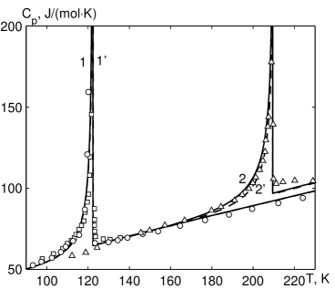
Figure 1: The temperature dependence of the molar specific heat of K(H_1-xD${}_{x})_{2}$PO₄ at $x=0.0$ — $\circ$ [18], $\square$ [19]; at $x=0.86$ — $\bigtriangleup$ [19]. Dashed lines 1’ and 2’: the theoretical results of [12].

In figures 3 and 3 we plotted the temperature variation of polarization of K(H_1-xD${}_{x})_{2}$PO₄ in different fields. The agreement with experiment is better at $x=0.89$ (and 0.84, see [17]) than at $x=0$. We believe this is due to proton tunnelling, essential in non-deuterated samples, which is not included in our model.

Figure 2: The temperature dependence of polarization of KH₂PO₄ at different $E_{3}$(MV/m): 0.0 — 1, $\vartriangle$ [5]; 0.581 — 2, $\circ$ [20]; 1.250 — 3, $\square$ [20]; 2.031 — 4, $\lozenge$ [20]. Symbols are experimental points; solid lines: the present theory; dashed lines: the theoretical results of [12].

Figure 3: The temperature dependence of polarization of K(H_1-xD${}_{x})_{2}$PO₄ at $x=0.89$ and at different $E_{3}$ (MV/m): 0.0 — 1; 0.282 — 2, $\circ$; 0.564 — 3, $\square$; 0.71 — 4; 0.846 — 5, $\lozenge$; 1.128 — 6, $\vartriangle$. Symbols are experimental points taken from [21]; lines: the present theory.

The field $E_{3}$, which in these crystals is the field conjugate to the order parameter, induces non-zero polarization $P_{3}$ above the transition point. Polarization has a jump at $T_{\textrm{c}}$, indicating the first order phase transition. With an increasing field, the polarization jump decreases, whereas the transition temperature $T_{\textrm{c}}$ increases almost linearly. The corresponding $\partial T_{\textrm{c}}/\partial E_{3}$ slopes are 0.192 and 0.115 K cm/kV for $x=0$ and $x=0.89$, respectively (c.f. 0.22 and 0.13 K cm/kV from our earlier calculations [10] and experimental $0.125$ K cm/kV of [23] for $x=0.89$). At some critical field $E^{*}$, the jump vanishes, and the transition smears out. The calculated coordinates of the critical point are $E^{*}=125$ V/cm, $T^{*}_{\textrm{c}}$=122.244 K for $x=0$ and $7.1$ kV/cm, 212.55 K for $x=0.89$, which agrees well with the experiment [22, 23]. It should be noted that in our previous calculations [12] it was impossible to obtain a correct description of the polarization behavior in the fields above the critical one, due to the necessity of using two different values of the effective dipole moment $\mu$ in calculations.

The calculated electrocaloric changes of temperature $\Delta T$ of the K(H_1-xD${}_{x})_{2}$PO₄ and K(H_1-xD${}_{x})_{2}$AsO₄ crystals with the adiabatically applied electric field are shown in figures 4 and 5. The experimental data of [7] were obtained at $T=121$ K, which was very close to the transition temperature of the sample used in the measurements.

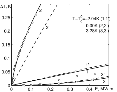
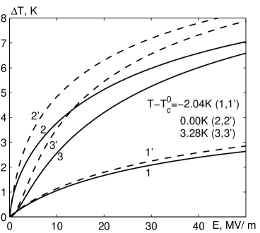
Figure 4: The field dependence of the electrocaloric temperature change of K(H_1-xD${}_{x})_{2}$PO₄ for $x=0.0$ (solid lines) and $x=0.89$ (dashed lines) at $T-T_{\textrm{c}}^{0}=-2.04$ K — 1, $1^{\prime}$, $\square$; $T=T_{\textrm{c}}^{0}$ — 2, $2^{\prime}$, $\circ$; $T-T_{\textrm{c}}^{0}=3.2$ K — 3, $3^{\prime}$, $\diamond$. Experimental points are taken from [5] — $\circ$, $\square$ and [7] — $\diamond$.

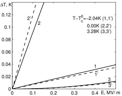
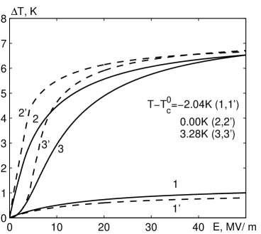
Figure 5: The field dependence of the electrocaloric temperature change of KH₂AsO₄ (solid lines) and KD₂AsO₄ (dashed lines) at $T-T_{\textrm{c}}^{0}=-2.04$ K — 1, $1^{\prime}$; $T=T_{\textrm{c}}^{0}$ — 2, $2^{\prime}$; $T-T_{\textrm{c}}^{0}=3.2$ K — 3, $3^{\prime}$.

As one can see, at small fields (figures 4, 5, left-hand) the calculated electrocaloric temperature change is a linear function of the field below $T_{\textrm{c}}^{0}$ (curves 1, $1^{\prime}$) and a quadratic function above $T_{\textrm{c}}^{0}$ (at 2, $2^{\prime}$). The experimental behavior below $T_{\textrm{c}}^{0}$ is not linear at $E_{3}<2$ kV/cm due to the domains: The domains, whose polarization is oriented along the field, are heated, whereas the domains, polarized in the opposite direction are cooled, thus the resulting net change of the sample temperature is close to zero. The experimental data for the electrocaloric temperature change at and above $T_{\textrm{c}}^{0}$ available for KH₂PO₄, as well as the $\Delta T/\Delta E$ ratio below $T_{\textrm{c}}^{0}$ at fields above 2 kV/cm (when the sample is in a single-domain state), are well reproduced by the theory.

At higher fields (figures 4, 5, right-hand) the calculated electrocaloric temperature changes at temperatures above $T_{\textrm{c}}^{0}$ are larger than below $T_{\textrm{c}}^{0}$. The obtained curves deviate from linear and quadratic behavior and reach saturation at $E\gg 500$ kV/cm. It should be mentioned, however, that these curves are calculated with the linear over the field $E_{3}$ pseudospin Hamiltonian (3). It would be very interesting to compare our results at high fields with experiment, for instance, to find out when non-linear contributions to the Hamiltonian cannot be omitted any longer. Unfortunately, no experimental data for $\Delta T$ in the fields above 1 kV/cm are available. And, of course, possibilities for experimental measurements are limited by the dielectric strength of the samples.

As one can see from the temperature dependence of $\Delta T$ (figure 6) for K(H_1-xD${}_{x})_{2}$PO₄ crystals, the calculated electrocaloric temperature change is the largest at temperatures below $T_{\textrm{c}}^{0}$ but close $T_{\textrm{c}}$ and can exceed 6 K; however, the fields required to reach $\Delta T$ that high are not accessible in reality, because most likely they exceed the dielectric strength of the crystals.

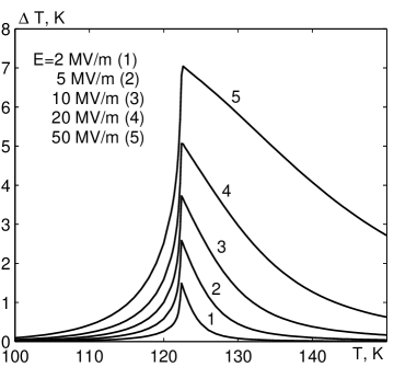
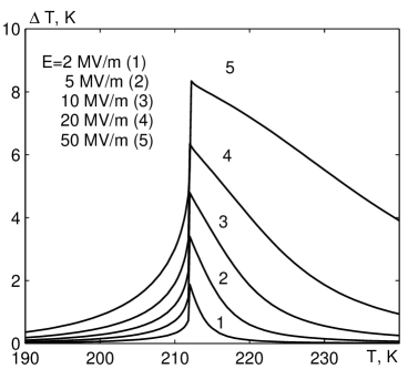
Figure 6: The temperature dependence of the electrocaloric temperature change of K(H_1-xD${}_{x})_{2}$PO₄ for $x=0.0$ (left-hand) and $x=0.89$ (right-hand) in different fields.

4 Conclusions

Taking into account the dependence of the effective dipole moment on the order parameter within the framework of the proton ordering model allows us to correctly describe the smearing of the ferroelectric phase transition in high electric fields as well as the electrocaloric effect in the KDP family crystals. The theory predicts the values of the electrocaloric temperature change of a few Kelvins in high fields. Additional experimental measurements of $\Delta T$ in the fields above 2 kV/cm are necessary.

Appendix

The notations introduced in equations (11)–(12) are as follows:

$$N_{6} = 2a(\beta\varepsilon)^{2}\cosh\beta\delta_{a}\varepsilon_{6}+4b(\beta w)^{2}\cosh(z-\beta\delta_{1}\varepsilon_{6})+(\beta w_{1})^{2}d+2\varepsilon_{6}\beta^{2}(-\varepsilon\delta_{a}M_{a}+w\delta_{1}M_{1})$$

$$+\,\varepsilon_{6}^{2}\left[2a(\beta\delta_{a})^{2}\cosh\beta\delta_{a}\varepsilon_{6}+(\beta\delta_{s})^{2}\cosh(2z+\beta\delta_{s}\varepsilon_{6})+4b(\beta\delta_{1})^{2}\cosh(z-\beta\delta_{1}\varepsilon_{6})\right],$$

$$q_{6}=2b\beta w\sinh(z-\beta\delta_{1}\varepsilon_{6})+\varepsilon_{6}\beta\left[-\delta_{s}\cosh(2z+\beta\delta_{s}\varepsilon_{6})+2b\delta_{1}\cosh(z-\beta\delta_{1}\varepsilon_{6})\right],$$

$$\lambda=-\beta\varepsilon\delta_{a}M_{a}+\beta w\delta_{1}M_{1}+\varepsilon_{6}\beta\left[\delta_{s}^{2}\cosh(2z+\beta\delta_{s}\varepsilon_{6})+2a\delta_{a}^{2}\cosh\beta\delta_{a}\varepsilon_{6}+4b\delta_{1}^{2}\cosh(z-\beta\delta_{1}\varepsilon_{6})\right],$$

$$\eta_{T}=p_{6}^{\varepsilon}+\frac{v}{2(\mu+12\mu^{\prime}\eta^{2})}(e_{36}-e_{36}^{2})\varepsilon_{T}\,,$$

$$\varepsilon_{T}=\left[\frac{2\beta}{vD}\left(2Tz_{T}f_{6}-\lambda+\frac{Mr}{D}\right)-\frac{4p_{6}^{\varepsilon}}{v}\left(\psi_{6}-\frac{z_{\eta}f_{6}}{D}\right)\right]\Big{/}c_{66}^{E}\,.$$

In turn,

$$p_{6}^{\varepsilon}=\frac{1}{T}\frac{2\varkappa Tz_{T}+[q_{6}-\eta M]}{D-2\varkappa z_{\eta}}\,,$$

$c_{66}^{E}$ is the isothermal elastic constant at a constant field

$$c_{66}^{E} = c_{66}^{E0}+\frac{8\psi_{6}}{v}\frac{\beta(-\psi_{6}\varkappa+f_{6})}{D-2z_{\eta}\varkappa}-\frac{4\beta z_{\eta}f_{6}^{2}}{vD(D-2z_{\eta}\varkappa)}$$

$$-\frac{2\beta}{vD}\left[\delta_{s}^{2}\cosh(2z+\beta\delta_{s}\varepsilon_{6})+2a\delta_{a}^{2}\cosh\beta\delta_{a}\varepsilon_{6}+4b\delta_{1}^{2}\cosh(z-\beta\delta_{1}\varepsilon_{6})\right]+\frac{2\beta r^{2}}{vD^{2}}\,,$$

and $e_{36}$ is the isothermal piezoelectric coefficient

$$e_{36}=-\left(\frac{\partial\sigma_{6}}{\partial E_{3}}\right)_{T,\varepsilon_{6}}=\left(\frac{\partial P_{3}}{\partial\varepsilon_{6}}\right)_{T,E_{3}}=e^{0}_{36}+\frac{2(\mu+12\mu^{\prime}\eta^{2})}{v}\frac{\beta\theta_{6}}{D-2z_{\eta}\varkappa}\,,$$

with

$$\theta_{6}=-2\varkappa\psi_{6}+f_{6}\,,\qquad f_{6}=\delta_{s}\cosh(2z+\beta\delta_{s}\varepsilon_{6})-2b\delta_{1}\cosh(z-\beta\delta_{1}\varepsilon_{6})+\eta r,$$

$$z_{\eta}=\frac{1}{1-\eta^{2}}+\beta\nu_{\textrm{c}}+12\beta\mu^{\prime}\eta E_{3}\,.$$

Ukrainian 0

Електрокалоричний ефект у кристалах типу KH₂PO₄ А.С. Вдович${}^{\textsf{\footnotesize{\mbox{?}}}}$, А.П. Моїна${}^{\textsf{\footnotesize{\mbox{?}}}}$, Р.Р. Левицький${}^{\textsf{\footnotesize{\mbox{?}}}}$, I.Р. Зачек${}^{\textsf{\footnotesize{\mbox{?}}}}$

             
${}^{\textsf{\footnotesize 1}}$ Iнститут фiзики конденсованих систем НАН України, вул. I. Свєнцiцького, 1, 79011 Львiв, Україна ${}^{\textsf{\footnotesize 2}}$ Нацiональний унiверситет ‘‘Львiвська полiтехнiка’’, вул. С. Бандери, 12, 79013 Львiв, Україна

References

• [1] Valant M., Progr. Mater. Sci., 2012, 57, 980; doi:10.1016/j.pmatsci.2012.02.001.
• [2] Scott J.F., Annu. Rev. Mater. Res., 2011, 41, 229; doi:10.1146/annurev-matsci-062910-100341.
• [3] Mischenko A.S., Zhang Q., Scott J.F., Whatmore R.W., Mathur N.D., Science, 2006, 311, 1270;
doi:10.1126/science.1123811.
• [4] Rose M.C., Cohen R.E., Phys. Rev. Lett., 2012, 109, 187604; doi:10.1103/PhysRevLett.109.187604.
• [5] Wiseman G.G., IEEE Trans. Electron Devices, 1969, 16, 588; doi:10.1109/T-ED.1969.16804.
• [6] Baumgartner H., Helv. Phys. Acta., 1950, 23, 651.
• [7] Shimshoni M., Harnik E., J. Phys. Chem. Solids, 1969, 31, 1416; doi:10.1016/0022-3697(70)90148-4.
• [8] Dunne L.J., Valant M., Manos G., Axelsson A.-K., Alford N., Appl. Phys. Lett., 2008, 93, 122906;
doi:10.1063/1.2991443.
• [9] Slater J.C., J. Chem. Phys., 1941, 9, 16; doi:10.1063/1.1750821.
• [10] Stasyuk I.V., Levitskii R.R., Moina A.P., Lisnii B.M., Ferroelectrics, 2001, 254, 213;
doi:10.1080/00150190108215002.
• [11] Stasyuk I.V., Levitskii R.R., Zachek I.R., Moina A.P., Phys. Rev. B, 2000, 62, 6198; doi:10.1103/PhysRevB.62.6198.
• [12] Levitsky R.R., Zachek I.R., Vdovych A.S., Moina A.P., J. Phys. Stud., 2010, 14, 1701.
• [13] Lisnii B.M., Levitskii R.R., Baran O.R., Phase Transitions, 2007, 80, 25; doi:10.1080/01411590701315591.
• [14] Stasyuk I.V., Levitskii R.R., Phys. Status Solidi B, 1970, 39, K35; doi:10.1002/pssb.19700390144.
• [15] Levitskii R.R., Korinevski N.A., Stasyuk I.V., Ukr. J. Phys., 1974, 19, 1289.
• [16] Blinc R., Svetina S., Phys. Rev., 1966, 147, 430; doi:10.1103/PhysRev.147.430.
• [17] Vdovych A.S., Moina A.P., Levitskii R.R., Zachek I.R., Preprint arXiv:1405.1327, 2014.
• [18] Stephenson C.C., Hooly G.J., J. Am. Chem. Soc., 1944, 66, No. 8, 1397; doi:10.1021/ja01236a054.
• [19] Strukov B.A., Baddur A., Koptsik V.A., Velichko I.A., Solid State Phys., 1972, 14, No. 4, 1034.
• [20] Chabin M., Gilletta F., Ferroelectrics, 1977, 15, 149; doi:10.1080/00150197708237808.
• [21] Sidnenko E.V., Gladkii V.V., Kristallografiya, 1972, 17, 978 (in Russian) [Sov. Phys. Crystallogr., 1973, 17, 861].
• [22] Western A.B., Baker A.G., Bacon C.R., Schmidt V.H., Phys. Rev. B, 1978, 17, 4461; doi:10.1103/PhysRevB.17.4461.
• [23] Gladkii V.V., Sidnenko E.V., Sov. Phys. Solid State, 1972, 13, 2592.
\@nopatterns
Ukrainian \adddialect\l@ukrainian0 \l@ukrainian