Towards a Learning Theory of Cause-Effect Inference

Abstract

We pose causal inference as the problem of learning to classify probability distributions. In particular, we assume access to a collection $\{(S_{i},l_{i})\}_{i=1}^{n}$, where each $S_{i}$ is a sample drawn from the probability distribution of $X_{i}\times Y_{i}$, and $l_{i}$ is a binary label indicating whether “$X_{i}\to Y_{i}$” or “$X_{i}\leftarrow Y_{i}$”. Given these data, we build a causal inference rule in two steps. First, we featurize each $S_{i}$ using the kernel mean embedding associated with some characteristic kernel. Second, we train a binary classifier on such embeddings to distinguish between causal directions. We present generalization bounds showing the statistical consistency and learning rates of the proposed approach, and provide a simple implementation that achieves state-of-the-art cause-effect inference. Furthermore, we extend our ideas to infer causal relationships between more than two variables.

1 Introduction

The vast majority of statistical learning algorithms rely on the exploitation of associations between the variables under study. Given the argument that all associations arise from underlying causal structures (Reichenbach, 1956), and that different structures imply different influences between variables, the question of how to infer and use causal knowledge in learning acquires great importance (Pearl, 2000; Schölkopf et al., 2012). Traditionally, the most widely used strategy to infer the causal structure of a system is to perform interventions on some of its variables, while studying the response of some others. However, such interventions are in many situations unethical, expensive, or even impossible to realize. Consequently, we often face the need of causal inference purely from observational data. In these scenarios, one suffers, in the absence of strong assumptions, from the indistinguishability between latent confounding ($X\leftarrow Z\rightarrow Y$) and direct causation ($X\to Y$ or $X\leftarrow Y$). Nevertheless, disregarding the impossibility of the task, humans continuously learn from experience to accurately infer causality-revealing patterns. Inspired by this successful learning, and in contrast to prior work, this paper addresses causal inference by unveiling such causal patterns directly from data. In particular, we assume access to a set $\{(S_{i},l_{i})\}_{i=1}^{n}$, where each $S_{i}$ is a sample set drawn from the probability distribution of $X_{i}\times Y_{i}$, and $l_{i}$ is a binary label indicating whether “$X_{i}\to Y_{i}$” or “$X_{i}\leftarrow Y_{i}$”. Using these data, we build a causal inference rule in two steps. First, we construct a suitable and nonparametric representation of each sample $S_{i}$. Second, we train a nonlinear binary classifier on such features to distinguish between causal directions. Building upon this framework, we derive theoretical guarantees regarding consistency and learning rates, extend inference to the multivariate case, propose approximations to scale learning to big data, and obtain state-of-the-art performance with a simple implementation.

Given the ubiquity of uncertainty in data, which may arise from noisy measurements or the existence of unobserved common causes, we adopt the probabilistic interpretation of causation from Pearl (2000). Under this interpretation, the causal structure underlying a set of random variables $X=(X_{1},\ldots,X_{d})$, with joint distribution $P$, is often described in terms of a Directed Acyclic Graph (DAG), denoted by $G=(V,E)$. In this graph, each vertex $V_{i}\in V$ is associated to the random variable $X_{i}\in X$, and an edge $E_{ji}\in E$ from $V_{j}$ to $V_{i}$ denotes the causal relationship “$X_{i}\leftarrow X_{j}$”. More specifically, these causal relationships are defined by a structural equation model: each $X_{i}\leftarrow f_{i}(\text{Pa}(X_{i}),N_{i})$, where $f_{i}$ is a function, $\text{Pa}(X_{i})$ is the parental set of $V_{i}\in V$, and $N_{i}$ is some independent noise variable. Then, causal inference is the task of recovering $G$ from $S\sim P^{n}$.

1.1 Prior Art

We now briefly review the state-of-the-art on the inference of causal structures $G$ from observational data $S\sim P^{n}$. For a more thorough exposition, see, e.g., Mooij et al. (2014).

One of the main strategies to recover $G$ is through the exploration of conditional dependencies, together with some other technical assumptions such as the Markov and faithfulness relationships between $P$ and $G$ (Pearl, 2000). This is the case of the PC algorithm (Spirtes et al., 2000), which allows the recovery of the Markov equivalence class of $G$ without placing any restrictions on the structural equation model specifying the random variables under study.

Causal inference algorithms that exploit conditional dependencies are unsuited for inference in the bivariate case. Consequently, a large body of work has been dedicated to the study of this scenario. First, the linear non-Gaussian causal model (Shimizu et al., 2006, 2011) recovers the true causal direction between two variables whenever their relationship is linear and polluted with additive and non-Gaussian noise. This model was later extended into nonlinear additive noise models (Hoyer et al., 2009; Zhang & Hyvärinen, 2009; Stegle et al., 2010; Kpotufe et al., 2013; Peters et al., 2014), which prefer the causal direction under which the alleged cause is independent from the additive residuals of some nonlinear fit to the alleged effect. Third, the information geometric causal inference framework (Daniusis et al., 2012; Janzing et al., 2014) assumes that the cause random variable is independently generated from some invertible and deterministic mapping to its effect; thus, it is unlikely to find dependencies between the density of the former and the slope of the latter, under the correct causal direction.

As it may be inferred from the previous exposition, there exists a large and heterogeneous array of causal inference algorithms, each of them working under a very specialized set of assumptions, which are sometimes difficult to test in practice. Therefore, there exists the need for a more flexible causal inference rule, capable of learning the relevant causal footprints, later used for inference, directly from data. Such a “data driven” approach would allow to deal with complex data-generating processes, and would greatly reduce the need of explicitly crafting identifiability conditions a-priori.

A preliminary step in this direction distilled from the competitions organized by Guyon (2013, 2014), which phrased causal inference as a learning problem. In these competitions, the participants were provided with a large collection of cause-effect samples $\{(S_{i},l_{i})\}_{i=1}^{n}$, where $S_{i}=\{(x_{ij},y_{ij})\}_{j=1}^{n_{i}}$ is drawn from the probability distribution of $X_{i}\times Y_{i}$, and $l_{i}$ is a binary label indicating whether “$X_{i}\to Y_{i}$” or “$Y_{i}\to X_{i}$”. Given these data, most participants adopted the strategy of i) crafting a vector of features from each $S_{i}$, and ii) training a binary classifier on top of the constructed features and paired labels. Although these “data-driven” methods achieved state-of-the-art performance (Guyon, 2013), the laborious task of hand-crafting features renders their theoretical analysis impossible.

In more specific terms, the approach described above is a learning problem with inputs being sample sets $S_{i}$, where each $S_{i}$ contains samples drawn from the probability distribution $P_{i}(X_{i},Y_{i})$. In a separate strand of research, there has been several attempts to learn from probability distributions in a principled manner (Jebara et al., 2004; Hein & Bousquet, 2004; Cuturi et al., 2005; Martins et al., 2009; Muandet et al., 2012). Szabó et al. (2014) presented the first theoretical analysis of distributional learning based on kernel mean embedding (Smola et al., 2007), with focus on kernel ridge regression. Similarly, Muandet et al. (2012) studied the problem of classifying distributions, but their approach is constrained to kernel machines, and no guarantees regarding consistency or learning rates are provided.

1.2 Our Contribution

Inspired by Guyon’s competitions, we pose causal inference as the problem of classifying probability measures on causally related pairs of random variables. Our contribution to this framework is the use of kernel mean embeddings to nonparametrically featurize each cause-effect sample $S_{i}$. The benefits of this approach are three-fold. First, this avoids the need of hand-engineering features from the samples $S_{i}$. Second, this enables a clean theoretical analysis, including provable learning rates and consistency results. Third, the kernel hyperparameters (that is, the data representation) can be jointly optimized with the classifier using cross-validation. Furthermore, we show how to extend these ideas to infer causal relationships between $d\geq 2$ variables, give theoretically sustained approximations to scale learning to big data, and provide the source code of a simple implementation that outperforms the state-of-the-art.

The rest of this article is organized as follows. Section 2 reviews the concept of kernel mean embeddings, the tool that will facilitate learning from distributions. Section 3 shows the consistency and learning rates of our kernel mean embedding classification approach to cause-effect inference. Section 4 extends the presented ideas to the multivariate causal inference case. Section 5 presents a variety of experiments displaying the state-of-the-art performance of a simple implementation of the proposed framework. For convenience, Table 1 summarizes our notations.

$\mathbb{E}[\xi],\mathbb{V}[\xi]$	Expected value and variance of r.v. $\xi$
$\mathcal{Z}$	Domain of cause-effect pairs $Z=(X,Y)$
$\mathcal{P}$	Set of cause-effect measures $P$ on $\mathcal{Z}$
$\mathcal{L}$	Set of labels $l_{i}\in\{-1,1\}$
$\mathscr{M}$	Mother distribution over $\mathcal{P}\times\mathcal{L}$
$\{(P_{i},l_{i})\}_{i=1}^{n}$	Sample from $\mathscr{M}^{n}$
$S_{i}\!=\!\{Z_{ij}\}_{j=1}^{n_{i}}$	Sample from $P_{i}^{n_{i}}$
$P_{S_{i}}$	Empirical distribution of $S_{i}$
$k$	Kernel function from $\mathcal{Z}\times\mathcal{Z}$ to $\mathbb{R}$
$\mathcal{H}_{k}$	RKHS induced by $k$
$\mu_{k}(P)$	Kernel mean embedding of measure $P\in\mathcal{P}$
$\mu_{k}(P_{s_{i}})$	Empirical mean embedding of $P_{s_{i}}$
$\mu_{k}(\mathcal{P})$	The set $\{\mu_{k}(P):P\in\mathcal{P}\}$
$\mathscr{M}_{k}$	Measure over $\mu_{k}(\mathcal{P})\times\mathcal{L}$ induced by $\mathscr{M}$
$\mathcal{F}_{k}$	Class of functionals mapping $\mathcal{H}_{k}$ to $\mathbb{R}$
$R_{n}(\mathcal{F}_{k})$	Rademacher complexity of class $\mathcal{F}_{k}$
$\varphi$, $R_{\varphi}(f)$	Cost and surrogate $\varphi$-risk of $\mathrm{sign}\circ\!f$

Table 1: Table of notations

2 Kernel Mean Embeddings of Probability Measures

In order to later classify probability measures $P$ according to their causal properties, we first need to featurize them into a suitable representation. To this end, we will rely on the concept of kernel mean embeddings (Berlinet & Thomas-Agnan, 2004; Smola et al., 2007).

In particular, let $P$ be the probability distribution of some random variable $Z$ taking values in the separable topological space $(\mathcal{Z},\tau_{z})$. Then, the kernel mean embedding of $P$ associated with the continuous, bounded, and positive-definite kernel function $k:\mathcal{Z}\times\mathcal{Z}\to\mathbb{R}$ is

$$\mu_{k}(P):=\int_{\mathcal{Z}}k(z,\cdot)\,\mathrm{d}P(z),$$ (1)

which is an element in $\mathcal{H}_{k}$, the Reproducing Kernel Hilbert Space (RKHS) associated with $k$ (Schölkopf & Smola, 2002). Interestingly, the mapping $\mu_{k}$ is injective if $k$ is a characteristic kernel (Sriperumbudur et al., 2010), that is, $\|\mu_{k}(P)-\mu_{k}(Q)\|_{\mathcal{H}_{k}}=0\Leftrightarrow P=Q$. Said differently, if using a characteristic kernel, we do not lose any information when embedding distributions. An example of characteristic kernel is the Gaussian kernel

$$k(z,z^{\prime})=\exp\left(-\gamma\|z-z^{\prime}\|_{2}^{2}\right),\,\,\gamma>0,$$ (2)

which will be used throughout this paper.

In many practical situations, it is unrealistic to assume access to the true distribution $P$, and consequently to the true embedding $\mu_{k}(P)$. Instead, we often have access to a sample $S=\{z_{i}\}_{i=1}^{n}\sim P^{n}$, which can be used to construct the empirical distribution $P_{S}:=\frac{1}{n}\sum_{z_{i}\in S}\delta_{(z_{i})}$, where $\delta_{(z)}$ is the Dirac distribution centered at $z$. Using $P_{S}$, we can approximate (1) by the empirical kernel mean embedding

$$\mu_{k}(P_{S}):=\frac{1}{n}\sum_{i=1}^{n}k(z_{i},\cdot)\in\mathcal{H}_{k}.$$ (3)

The following result is a slight modification of Theorem 27 from (Song, 2008). It establishes the convergence of the empirical mean embedding $\mu_{k}(P_{S})$ to the embedding of its population counterpart $\mu_{k}(P)$, in RKHS norm:

Theorem 1.

Assume that $\|f\|_{\infty}\leq 1$ for all $f\in\mathcal{H}_{k}$ with $\|f\|_{\mathcal{H}_{k}}\leq 1$. Then with probability at least $1-\delta$ we have

$$\|\mu_{k}(P)-\mu_{k}(P_{S})\|_{\mathcal{H}_{k}}\leq 2\sqrt{\frac{\operatorname*{\mathbb{E}\,}_{z\sim P}[k(z,z)]}{n}}+\sqrt{\frac{2\log\frac{1}{\delta}}{n}}.$$

Proof.

See Section B.1.∎

3 A Theory of Causal Inference as Distribution Classification

This section phrases the inference of cause-effect relationships from probability measures as the classification of empirical kernel mean embeddings, and analyzes the learning rates and consistency of such approach. Throughout our exposition, the setup is as follows:

1. We assume the existence of some Mother distribution $\mathscr{M}$, defined on $\mathcal{P}\times\mathcal{L}$, where $\mathcal{P}$ is the set of all Borel probability measures on the space $\mathcal{Z}$ of two causally related random variables, and $\mathcal{L}=\{-1,+1\}$.

2. A set $\{(P_{i},l_{i})\}_{i=1}^{n}$ is sampled from $\mathscr{M}^{n}$. Each measure $P_{i}\in\mathcal{P}$ is the joint distribution of the causally related random variables $Z_{i}=(X_{i},Y_{i})$, and the label $l_{i}\in\mathcal{L}$ indicates whether “$X_{i}\to Y_{i}$” or “$X_{i}\leftarrow Y_{i}$”.

3. In practice, we do not have access to the measures $\{P_{i}\}_{i=1}^{n}$. Instead, we observe samples $S_{i}=\{(x_{ij},y_{ij})\}_{j=1}^{n_{i}}\sim P_{i}^{n_{i}}$, for all $1\leq i\leq n$. Using $S_{i}$, the data $\{(S_{i},l_{i})\}_{i=1}^{n}$ is provided to the learner.

4. We featurize every sample $S_{i}$ into the empirical kernel mean embedding $\mu_{k}(P_{S_{i}})$ associated with some kernel function $k$ (Equation 3). If $k$ is a characteristic kernel, we incur no loss of information in this step.

Under this setup, we will use the set $\{(\mu_{k}(P_{S_{i}}),l_{i})\}_{i=1}^{n}$ to train a binary classifier from $\mathcal{H}_{k}$ to $\mathcal{L}$, which will later be used to unveil the causal directions of new, unseen probability measures drawn from $\mathscr{M}$. Note that this framework can be straightforwardly extended to also infer the “confounding ($X\leftarrow Z\rightarrow Y$)” and “independent ($X\mathrel{\text{\scalebox{1.07}{$\perp\mkern-10.0mu\perp$}}}Y$)” cases by adding two extra labels to $\mathcal{L}$.

Given the two nested levels of sampling (being the first one from the Mother distribution $\mathscr{M}$, and the second one from each of the drawn cause-effect measures $P_{i}$), it is not trivial to conclude whether this learning procedure is consistent, or how its learning rates depend on the sample sizes $n$ and $\{n_{i}\}_{i=1}^{n}$. In the following, we will study the generalization performance of empirical risk minimization over this learning setup. Specifically, we are interested in upper bounding the excess risk between the empirical risk minimizer and the best classifier from our hypothesis class, with respect to the Mother distribution $\mathscr{M}$.

We divide our analysis in three parts. First, §3.1 reviews the abstract setting of statistical learning theory and surrogate risk minimization. Second, §3.2 adapts these standard results to the case of empirical kernel mean embedding classification. Third, §3.3 considers theoretically sustained approximations to deal with big data.

3.1 Margin-based Risk Bounds in Learning Theory

Let $\mathbb{P}$ be some unknown probability measure defined on $\mathcal{Z}\times\mathcal{L}$, where $\mathcal{Z}$ is referred to as the input space, and $\mathcal{L}=\{-1,1\}$ is referred to as the output space. One of the main goals of statistical learning theory (Vapnik, 1998) is to find a classifier $h\colon\mathcal{Z}\to\mathcal{L}$ that minimizes the expected risk

$$R(h)=\operatorname*{\mathbb{E}\,}_{(z,l)\sim\mathbb{P}}\bigl{[}\ell\bigl{(}h(z),l\bigr{)}\bigr{]}$$

for a suitable loss function $\ell\colon\mathcal{L}\times\mathcal{L}\to\mathbb{R}^{+}$, which penalizes departures between predictions $h(z)$ and true labels $l$. For classification, one common choice of loss function is the 0-1 loss $\ell_{01}(l,l^{\prime})=|l-l^{\prime}|$, for which the expected risk measures the probability of misclassification. Since $\mathbb{P}$ is unknown in natural situations, one usually resorts to the minimization of the empirical risk $\frac{1}{n}\sum_{i=1}^{n}\ell\bigl{(}h(z_{i}),l_{i}\bigr{)}$ over some fixed hypothesis class $\mathcal{H}$, for the training set $\{(z_{i},l_{i})\}_{i=1}^{n}\sim\mathbb{P}^{n}$. It is well known that this procedure is consistent under mild assumptions (Boucheron et al., 2005).

Unfortunately, the 0-1 loss function is not convex, which leads to empirical risk minimization being generally intractable. Instead, we will focus on the minimization of surrogate risk functions (Bartlett et al., 2006). In particular, we will consider the set of classifiers of the form $\mathcal{H}=\{{\mathrm{sign}\circ\!f}\colon{f\in\mathcal{F}}\}$ where $\mathcal{F}$ is some fixed set of real-valued functions ${f\colon\mathcal{Z}\to\mathbb{R}}$. Introduce a nonnegative cost function $\varphi\colon\mathbb{R}\to\mathbb{R}^{+}$ which is surrogate to the 0-1 loss, that is, $\varphi(\epsilon)\geq\mathbbm{1}_{\epsilon>0}$. For any $f\in\mathcal{F}$ we define its expected and empirical $\varphi$-risks respectively as

$$R_{\varphi}(f)=\operatorname*{\mathbb{E}\,}_{(z,l)\sim\mathbb{P}}\bigl{[}\varphi\bigl{(}-f(z)l\bigr{)}\bigr{]},$$ (4)

$$\hat{R}_{\varphi}(f)=\frac{1}{n}\sum_{i=1}^{n}\varphi\bigl{(}-f(z_{i})l_{i}\bigr{)}.$$ (5)

Many natural choices of $\varphi$ lead to tractable empirical risk minimization. Common examples of cost functions include the hinge loss $\varphi(\epsilon)=\max(0,1+\epsilon)$ used in SVM, the exponential loss $\varphi(\epsilon)=\exp(\epsilon)$ used in Adaboost, and the logistic loss $\varphi(\epsilon)=\log_{2}\bigl{(}1+e^{\epsilon})$ used in logistic regression.

The misclassification error of $\mathrm{sign}\circ\!f$ is always upper bounded by $R_{\varphi}(f)$. The relationship between functions minimizing $R_{\varphi}(f)$ and functions minimizing ${R(\mathrm{sign}\circ\!f)}$ has been intensively studied in the literature (Steinwart & Christmann, 2008, Chapter 3). Given the high uncertainty associated with causal inferences, we argue that one is interested in predicting soft probabilities rather than hard labels, a fact that makes the study of margin-based classifiers well suited for our problem.

We now focus on the estimation of $f^{*}\in\mathcal{F}$, the function minimizing (4). However, since the distribution $\mathbb{P}$ is unknown, we can only hope to estimate $\hat{f}_{n}\in\mathcal{F}$, the function minimizing (5). Therefore, we are interested in high-probability upper bounds on the excess $\varphi$-risk

$$\mathcal{E}_{\mathcal{F}}(\hat{f}_{n})=R_{\varphi}(\hat{f}_{n})-R_{\varphi}(f^{*}),$$ (6)

w.r.t. the random training sample $\{(z_{i},l_{i})\}_{i=1}^{n}\sim\mathbb{P}^{n}$. The excess risk (6) can be upper bounded in the following way:

$$\mathcal{E}_{\mathcal{F}}(\hat{f}_{n}) \leq R_{\varphi}(\hat{f}_{n})-\hat{R}_{\varphi}(\hat{f}_{n})+\hat{R}_{\varphi}(f^{*})-R_{\varphi}(f^{*})$$

$$\leq 2\sup_{f\in\mathcal{F}}|R_{\varphi}(f)-\hat{R}_{\varphi}(f)|.$$ (7)

While this upper bound leads to tight results for worst case analysis, it is well known (Bartlett et al., 2005; Boucheron et al., 2005; Koltchinskii, 2011) that tighter bounds can be achieved under additional assumptions on $\mathbb{P}$. However, we leave these analyses for future research.

The following result — in spirit of Koltchinskii & Panchenko (1999); Bartlett & Mendelson (2002) — can be found in Boucheron et al. (2005, Theorem 4.1).

Theorem 2.

Consider a class $\mathcal{F}$ of functions mapping $\mathcal{Z}$ to $\mathbb{R}$. Let $\varphi\colon\mathbb{R}\to\mathbb{R}^{+}$ be a $L_{\varphi}$-Lipschitz function such that $\varphi(\epsilon)\geq\mathbbm{1}_{\epsilon>0}$. Let $B$ be a uniform upper bound on $\varphi\bigl{(}-f(\epsilon)l\bigr{)}$. Let $\{(z_{i},l_{i})\}_{i=1}^{n}\sim\mathbb{P}$ and $\{\sigma_{i}\}_{i=1}^{n}$ be i.i.d. Rademacher random signs. Then, with prob. at least $1-\delta$,

$$\sup_{f\in\mathcal{F}}|R_{\varphi}(f)-\hat{R}_{\varphi}(f)|\\ \leq 2L_{\varphi}\operatorname*{\mathbb{E}\,}\left[\sup_{f\in\mathcal{F}}\frac{1}{n}\left|\sum_{i=1}^{n}\sigma_{i}f(z_{i})\right|\right]+B\sqrt{\frac{\log(1/\delta)}{2n}},$$

where the expectation is taken w.r.t. $\{\sigma_{i},z_{i}\}_{i=1}^{n}$.

The expectation in the bound of Thm. 2 is known as the Rademacher complexity of $\mathcal{F}$, will be denoted by $R_{n}(\mathcal{F})$, and has a typical order of $O(n^{-1/2})$ (Koltchinskii, 2011).

3.2 From Classic to Distributional Learning Theory

Note that we can not directly apply the empirical risk minimization bounds discussed in the previous section to our learning setup. This is because instead of learning a classifier on the i.i.d. sample $\{\mu_{k}(P_{i}),l_{i}\}_{i=1}^{n}$, we have to learn over the set $\{\mu_{k}(P_{S_{i}}),l_{i}\}_{i=1}^{n}$, where $S_{i}\sim P_{i}^{n_{i}}$. Said differently, our input feature vectors $\mu_{k}(P_{S_{i}})$ are “noisy”: they exhibit an additional source of variation as any two different random samples $S_{i},S_{i}^{\prime}\sim P_{i}^{n_{i}}$ do. In the following, we study how to incorporate these nested sampling effects into an argument similar to Theorem 2.

We will now frame our problem within the abstract learning setting considered in the previous section. Recall that our learning setup initially considers some Mother distribution $\mathscr{M}$ over $\mathcal{P}\times\mathcal{L}$. Let $\mu_{k}(\mathcal{P})=\{\mu_{k}(P):P\in\mathcal{P}\}\subseteq\mathcal{H}_{k}$, $\mathcal{L}=\{-1,+1\}$, and $\mathscr{M}_{k}$ be a measure (guaranteed to exist by Lemma 2, Section A.1) on $\mu_{k}(\mathcal{P})\times\mathcal{L}$ induced by $\mathscr{M}$. Specifically, we will consider $\mu_{k}(\mathcal{P})\subseteq\mathcal{H}_{k}$ and $\mathcal{L}$ to be the input and output spaces of our learning problem, respectively. Let $\bigl{\{}\bigl{(}\mu_{k}(P_{i}),l_{i}\bigr{)}\bigr{\}}_{i=1}^{n}\sim\mathscr{M}_{k}^{n}$ be our training set. We will now work with the set of classifiers $\{\mathrm{sign}\circ\!f\colon f\in\mathcal{F}_{k}\}$ for some fixed class $\mathcal{F}_{k}$ of functionals mapping from the RKHS $\mathcal{H}_{k}$ to $\mathbb{R}$.

As pointed out in the description of our learning setup, we do not have access to the distributions $\{P_{i}\}_{i=1}^{n}$ but to samples $S_{i}\sim P_{i}^{n_{i}}$, for all $1\leq i\leq n$. Because of this reason, we define the sample-based empirical $\varphi$-risk

$$\tilde{R}_{\varphi}(f)=\frac{1}{n}\sum_{i=1}^{n}\varphi\bigl{(}-l_{i}f\bigl{(}\mu_{k}(P_{S_{i}})\bigr{)}\bigr{)},$$

which is the approximation to the empirical $\varphi$-risk $\hat{R}_{\varphi}(f)$ that results from substituting the embeddings $\mu_{k}(P_{i})$ with their empirical counterparts $\mu_{k}(P_{S_{i}})$.

Our goal is again to find the function $f^{*}\in\mathcal{F}_{k}$ minimizing expected $\varphi$-risk $R_{\varphi}(f)$. Since $\mathscr{M}_{k}$ is unknown to us, and we have no access to the embeddings $\{\mu_{k}(P_{i})\}_{i=1}^{n}$, we will instead use the minimizer of $\tilde{R}_{\varphi}(f)$ in $\mathcal{F}_{k}$:

$$\tilde{f}_{n}\in\arg\min_{f\in\mathcal{F}_{k}}\tilde{R}_{\varphi}(f).$$ (8)

To sum up, the excess risk (6) can now be reformulated as

$$R_{\varphi}(\tilde{f}_{n})-R_{\varphi}(f^{*}).$$ (9)

Note that the estimation of $f^{*}$ drinks from two nested sources of error, which are i) having only $n$ training samples from the distribution $\mathscr{M}_{k}$, and ii) having only $n_{i}$ samples from each measure $P_{i}$. Using a similar technique to (7), we can upper bound the excess risk as

$$R_{\varphi}(\tilde{f}_{n})-R_{\varphi}(f^{*}) \leq\sup_{f\in\mathcal{F}_{k}}|R_{\varphi}(f)-\hat{R}_{\varphi}(f)|$$ (10)

$$+\sup_{f\in\mathcal{F}_{k}}|\hat{R}_{\varphi}(f)-\tilde{R}_{\varphi}(f)|.$$ (11)

The term (10) is upper bounded by Theorem 2. On the other hand, to deal with (11), we will need to upper bound the deviations $\bigl{|}f\bigl{(}\mu_{k}(P_{i})\bigr{)}-f\bigl{(}\mu_{k}(P_{S_{i}})\bigr{)}\bigr{|}$ in terms of the distances $\|\mu_{k}(P_{i})-\mu_{k}(P_{S_{i}})\|_{\mathcal{H}_{k}}$, which are in turn upper bounded using Theorem 1. To this end, we will have to assume that the class $\mathcal{F}_{k}$ consists of functionals with uniformly bounded Lipschitz constants, such as the set of linear functionals with uniformly bounded operator norm.

We now present the main result of this section, which provides a high-probability bound on the excess risk (9). Importantly, this excess risk will translate into the expected causal inference accuracy of our distribution classifier.

Theorem 3.

Consider the RKHS $\mathcal{H}_{k}$ associated with some bounded, continuous kernel function $k$, such that $\sup_{z\in\mathcal{Z}}k(z,z)\leq 1$. Consider a class $\mathcal{F}_{k}$ of functionals mapping $\mathcal{H}_{k}$ to $\mathbb{R}$ with Lipschitz constants uniformly bounded by $L_{\mathcal{F}}$. Let $\varphi\colon\mathbb{R}\to\mathbb{R}^{+}$ be a $L_{\varphi}$-Lipschitz function such that $\phi(z)\geq\mathbbm{1}_{z>0}$. Let $\varphi\bigl{(}-f(h)l\bigr{)}\leq B$ for every $f\in\mathcal{F}_{k}$, $h\in\mathcal{H}_{k}$, and $l\in\mathcal{L}$. Then, with probability not less than $1-\delta$ (over all sources of randomness)

$$R_{\varphi}(\tilde{f}_{n})-R_{\varphi}(f^{*})\leq 4L_{\varphi}R_{n}(\mathcal{F}_{k})+2B\sqrt{\frac{\log(2/\delta)}{2n}}$$

$$+\frac{4L_{\varphi}L_{\mathcal{F}}}{n}\sum_{i=1}^{n}\left(\sqrt{\frac{\operatorname*{\mathbb{E}\,}_{z\sim P_{i}}[k(z,z)]}{n_{i}}}+\sqrt{\frac{\log(2n/\delta)}{2n_{i}}}\right).$$

Proof.

See Section B.2.∎

As mentioned in Section 3.1, the typical order of $R_{n}(\mathcal{F}_{k})$ is $O(n^{-1/2})$. For a particular examples of classes of functionals with small Rademacher complexity we refer to Maurer (2006). In such cases, the upper bound in Theorem 3 converges to zero (meaning that our procedure is consistent) as both $n$ and $n_{i}$ tend to infinity, in such a way that $\log n/n_{i}=o(1)$. The rate of convergence w.r.t. $n$ can be improved up to $O(n^{-1})$ if placing additional assumptions on $\mathscr{M}$ (Bartlett et al., 2005). On the contrary, the rate w.r.t. $n_{i}$ cannot be improved in general. Namely, the convergence rate $O(n^{-1/2})$ presented in the upper bound of Theorem 1 is tight, as shown in the following novel result.

Theorem 4.

Under the assumptions of Theorem 1 denote

$$\sigma^{2}_{\mathcal{H}_{k}}=\sup_{\|f\|_{\mathcal{H}_{k}}\leq 1}\mathbb{V}_{z\sim P}[f(z)].$$

Then there exist universal constants $c,C$ such that for every integer $n\geq 1/\sigma^{2}_{\mathcal{H}_{k}}$, and with probability at least $c$

$$\|\mu_{k}(P)-\mu_{k}(P_{S})\|_{\mathcal{H}_{k}}\geq C\frac{\sigma_{\mathcal{H}_{k}}}{\sqrt{n}}.$$

Proof.

See Section B.3.∎

Finally, it is instructive to relate the notion of “identifiability” often considered in the causal inference community (Pearl, 2000) to the properties of the Mother distribution. Saying that the model is identifiable means that the label $l$ of $P\in\mathcal{P}$ is assigned deterministically by $\mathscr{M}$. In this case, learning rates can become as fast as $O(n^{-1})$. On the other hand, as $\mathscr{M}(l|P)$ becomes nondeterministic, the problem becomes unidentifiable and learning rates slow down (for example, in the extreme case of cause-effect pairs related by linear functions polluted with additive Gaussian noise, $\mathscr{M}(l=+1|P)=\mathscr{M}(l=-1|P)$ almost surely). The investigation of these phenomena is left for future research.

3.3 Low Dimensional Embeddings for Large Data

For some kernel functions, the embeddings $\mu_{k}(P_{S})\in\mathcal{H}_{k}$ are infinite dimensional. Because of this reason, one must resort to the use of dual optimization problems, and in particular, kernel matrices. The construction of these matrices requires at least $O(n^{2})$ computational and memory requirements, prohibitive for large $n$. In this section, we show that the infinite-dimensional embeddings $\mu_{k}(P_{S})\in\mathcal{H}_{k}$ can be approximated with easy to compute, low-dimensional representations (Rahimi & Recht, 2007, 2008). This will allow us to replace the infinite-dimensional minimization problem (8) with a low-dimensional one.

Assume that $\mathcal{Z}=\mathbb{R}^{d}$, and that the kernel function $k$ is real-valued, and shift-invariant. Then, we can exploit Bochner’s theorem (Rudin, 1962) to show that, for any $z,z^{\prime}\in\mathcal{Z}$:

$$k(z,z^{\prime})\!=2C_{k}\!\operatorname*{\mathbb{E}\,}_{w,b}\!\left[\cos(\langle w,z\rangle\!+b)\cos(\langle w,z^{\prime}\rangle\!+b)\right],$$ (12)

where $w\sim\frac{1}{C_{k}}p_{k}$, $b\sim\mathcal{U}[0,2\pi]$, $p_{k}\colon\mathcal{Z}\to\mathbb{R}$ is the positive and integrable Fourier transform of $k$, and $C_{k}=\int_{\mathcal{Z}}p_{k}(w)dw$. For example, the squared-exponential kernel (2) is shift-invariant, and its evaluations can be approximated by (12), if setting $p_{k}(w)=\mathcal{N}(w|0,2\gamma I)$, and $C_{k}=1$.

We now show that for any probability measure $Q$ on $\mathcal{Z}$ and $z\in\mathcal{Z}$, the function $k(z,\cdot)\in\mathcal{H}_{k}\subseteq L_{2}(Q)$ can be approximated by a linear combination of randomly chosen elements from the Hilbert space $L_{2}(Q)$. Namely, consider the functions parametrised by $w,z\in\mathcal{Z}$ and $b\in[0,2\pi]$:

$$g_{w,b}^{z}(\cdot)=2C_{k}\cos(\langle w,z\rangle+b)\cos(\langle w,\cdot\rangle+b),$$ (13)

which belong to $L_{2}(Q)$, since they are bounded. If we sample $\{(w_{j},b_{j})\}_{j=1}^{m}$ i.i.d., as discussed above, the average

$$\hat{g}_{m}^{z}(\cdot)=\frac{1}{m}\sum_{i=1}^{m}g_{w_{i},b_{i}}^{z}(\cdot)$$

can be viewed as an $L_{2}(Q)$-valued random variable. Moreover, (12) shows that $\operatorname*{\mathbb{E}\,}_{w,b}[\hat{g}_{m}^{z}(\cdot)]=k(z,\cdot)$. This enables us to invoke concentration inequalities for Hilbert spaces (Ledoux & Talagrand, 1991), to show the following result, which is in spirit to Rahimi & Recht (2008, Lemma 1).

Lemma 1.

Let $\mathcal{Z}=\mathbb{R}^{d}$. For any shift-invariant kernel $k$, s.t. $\sup_{z\in\mathcal{Z}}k(z,z)\leq 1$, any fixed $S=\{z_{i}\}_{i=1}^{n}\subset\mathcal{Z}$, any probability distribution $Q$ on $\mathcal{Z}$, and any $\delta>0$, we have

$$\Biggl{\|}\mu_{k}(P_{S})-\frac{1}{n}\sum_{i=1}^{n}\hat{g}_{m}^{z_{i}}(\cdot)\Biggr{\|}_{L_{2}(Q)}\!\!\!\!\!\leq\frac{2C_{k}}{\sqrt{m}}\left(1+\sqrt{{2\log(n/\delta)}}\right)$$

with probability larger than $1-\delta$ over $\{(w_{i},b_{i})\}_{i=1}^{m}$.

Proof.

See Section B.4.∎

Once sampled, the parameters $\{(w_{i},b_{i})\}_{i=1}^{m}$ allow us to approximate the empirical kernel mean embeddings $\{\mu_{k}(P_{S_{i}})\}_{i=1}^{n}$ using elements from $\text{span}({\{\cos(\langle w_{i},\cdot\rangle+b_{i})\}_{i=1}^{m}})$, which is a finite-dimensional subspace of $L_{2}(Q)$. Therefore, we propose to use $\{(\mu_{k,m}(P_{S_{i}}),l_{i})\}_{i=1}^{n}$ as the training sample for our final empirical risk minimization problem, where

$$\mu_{k,m}(P_{S})=\frac{2C_{k}}{|S|}\sum_{z\in S}\bigl{(}\cos(\langle w_{j},z\rangle+b_{j})\bigr{)}_{j=1}^{m}\!\!\in\!\mathbb{R}^{m}.$$ (14)

These feature vectors can be computed in $O(m)$ time and stored in $O(1)$ memory; importantly, they can be used off-the-shelf in conjunction with any learning algorithm.

For the precise excess risk bounds that take into account the use of these low-dimensional approximations, please refer to Theorem 6 from Section B.5.

4 Extensions to Multivariate Causal Inference

It is possible to extend our framework to infer causal relatonships between $d\geq 2$ variables $X=(X_{1},\ldots,X_{d})$. To this end, and as introduced in Section 1, assume the existence of a causal directed acyclic graph $G$ which underlies the dependencies present in the probability distribution $P(X)$. Therefore, our task is to recover $G$ from $S\sim P^{n}$.

Naïvely, one could extend the framework presented in Section 3 from the binary classification of $2$-dimensional distributions to the multiclass classification of $d$-dimensional distributions. However, the number of possible DAGs (and therefore, the number of labels in our multiclass classification problem) grows super-exponentially in $d$.

An alternative approach is to consider the probabilities of the three labels “$X_{i}\to X_{j}$”, “$X_{i}\leftarrow X_{j}$“, and “$X_{i}\mathrel{\text{\scalebox{1.07}{$\perp\mkern-10.0mu\perp$}}}X_{j}$“ for each pair of variables $\{X_{i},X_{j}\}\subseteq X$, when embedded along with every possible context $X_{k}\subseteq X\setminus\{X_{i},X_{j}\}$. The intuition here is the same as in the PC algorithm of Spirtes et al. (2000): in order to decide the (absence of a) causal relationship between $X_{i}$ and $X_{j}$, one must analyze the confounding effects of every $X_{k}\subseteq X\setminus\{X_{i},X_{j}\}$.

5 Numerical Simulations

We conduct an array of experiments to test the effectiveness of a simple implementation of the presented causal learning framework. Given the use of random embeddings (14) in our classifier, we term our method the Randomized Causation Coefficient (RCC). Throughout our simulations, we featurize each sample $S=\{(x_{i},y_{i})\}_{i=1}^{n}$ as

$$\nu(S)=(\mu_{k,m}(P_{S_{x}}),\mu_{k,m}(P_{S_{y}}),\mu_{k,m}(P_{S_{xy}})),$$ (15)

where the three elements forming (15) stand for the low-dimensional representations (14) of the empirical kernel mean embeddings of $\{x_{i}\}_{i=1}^{n}$, $\{y_{i}\}_{i=1}^{n}$, and $\{(x_{i},y_{i})\}_{i=1}^{n}$, respectively. The representation (15) is motivated by the typical conjecture in causal inference about the existence of asymmetries between the marginal and conditional distributions of causally-related pairs of random variables (Schölkopf et al., 2012). Each of these three embeddings has random features sampled to approximate the sum of three Gaussian kernels (2) with hyper-parameters $0.1\gamma$, $\gamma$, and $10\gamma$, where $\gamma$ is found using the median heuristic. In practice, we set $m=1000$, and observe no significant improvements when using larger amounts of random features. To classify the embeddings (15) in each of the experiments, we use the random forest implementation from Python’s sklearn-0.16-git. The number of trees is chosen from $\{100,250,500,1000,5000\}$ via cross-validation.

Our experiments can be replicated using the source code at

https://github.com/lopezpaz/causation_learning_theory.

5.1 Classification of Tübingen Cause-Effect Pairs

The Tübingen cause-effect pairs is a collection of heterogeneous, hand-collected, real-world cause-effect samples (Zscheischler, 2014). Given the small size of this dataset, we resort to the synthesis of an artificial Mother distribution to sample our training data from. To this end, assume that sampling a synthetic cause-effect sample set $\hat{S}_{i}:=\{(\hat{x}_{ij},\hat{y}_{ij})\}_{j=1}^{n}\sim{\mathcal{P}}_{\theta}$ equals the following simple generative process:

1. A cause vector $(\hat{x}_{ij})_{j=1}^{n}$ is sampled from a mixture of Gaussians with $c$ components. The mixture weights are sampled from $\mathcal{U}(0,1)$, and normalized to sum to one. The mixture means and standard deviations are sampled from $\mathcal{N}(0,\sigma_{1})$, and $\mathcal{N}(0,\sigma_{2})$, respectively, accepting only positive standard deviations. The cause vector is standardized to zero mean and unit variance.

2. A noise vector $(\hat{\epsilon}_{ij})_{j=1}^{n}$ is sampled from a centered Gaussian, with variance sampled from $\mathcal{U}(0,\sigma_{3})$.

3. A mapping mechanism $\hat{f}_{i}$ is conceived as a spline fitted using an uniform grid of $d_{f}$ elements from $\min((\hat{x}_{ij})_{j=1}^{n})$ to $\max((\hat{x}_{ij})_{j=1}^{n})$ as inputs, and $d_{f}$ normally distributed outputs.

4. An effect vector is built as $(\hat{y}_{ij}:=\hat{f}_{i}(\hat{x}_{ij})+\hat{\epsilon}_{ij})_{j=1}^{n}$, and standardized to zero mean and unit variance.

5. Return the cause-effect sample $\hat{S}_{i}:=\{(\hat{x}_{ij},\hat{y}_{ij})\}_{j=1}^{n}$.

To choose a $\theta=(c,\sigma_{1},\sigma_{2},\sigma_{3},d_{f})$ that best resembles the unlabeled test data, we minimize the distance between the embeddings of $N$ synthetic pairs and the Tuebingen samples

$$\operatorname*{arg\,min}_{\theta}\sum_{i}\min_{1\leq j\leq N}\|\nu(S_{i})-\nu(\hat{S}_{j})\|^{2}_{2},$$ (16)

over $c,d_{f}\in\{1,\ldots,10\}$, and $\sigma_{1},\sigma_{2}$, and $\sigma_{3}\in\{0,0.5,1,\ldots,5\}$, where the $\hat{S}_{j}\sim\mathcal{P}_{\theta}$, the $S_{i}$ are the Tübingen cause-effect pairs, and $\nu$ is as in (15). This strategy can be thought of as transductive learning, since we assume to know the test inputs prior to the training of our inference rule. We set $n=1000$, and $N=10,000$.

Using the generative process outlined above, we construct the synthetic training data

$$\{ \{\nu(\{(\hat{x}_{ij},\hat{y}_{ij})\}_{j=1}^{n}),+1)\}_{i=1}^{N},$$

$$\{\nu(\{(\hat{y}_{ij},\hat{x}_{ij})\}_{j=1}^{n}),-1)\}_{i=1}^{N}\},$$

where $\{(\hat{x}_{ij},\hat{y}_{ij})\}_{j=1}^{n}\sim\mathcal{P}_{\theta}$, and train our classifier on it.

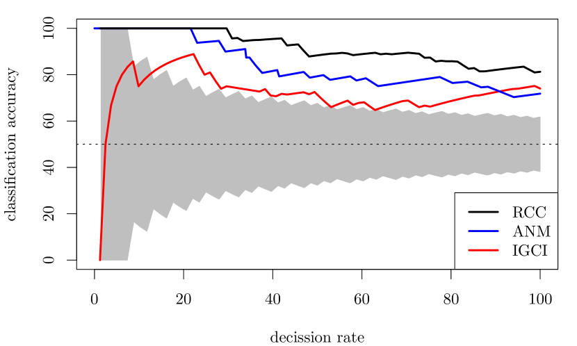
Figure 1: Accuracy of RCC, IGCI and ANM on the Tübingen cause-effect pairs, as a function of decision rate. The grey area depicts accuracies not statistically significant.

Figure 1 plots the classification accuracy of RCC, IGCI (Daniusis et al., 2012), and ANM (Mooij et al., 2014) versus the fraction of decissions that the algorithms are forced to make out of the 82 scalar Tüebingen cause-effect pairs. To compare these results to other lower-performing methods, refer to Janzing et al. (2012). RCC surpasses the state-of-the-art with a classification accuracy of $81.61\%$ when inferring the causal directions on all pairs. The confidence of RCC is computed using the classifier’s output class probabilities. SVMs obtain a test accuracy of $77.2\%$ in this same task.

5.2 Inferring the Arrow of Time

We test the effectiveness of our method to infer the arrow of time from causal time series. More specifically, we assume access to a set of time series $\{x_{ij}\}_{j=1}^{n_{i}}$, and our task is to infer, for each series, whether $X_{i}\to X_{i+1}$ or $X_{i}\leftarrow X_{i+1}$.

We compare our framework to the state-of-the-art of Peters et al. (2009), using the same electroencephalography signals (Blankertz, 2005) as in their original experiment. On the one hand, Peters et al. (2009) construct two Auto-Regressive Moving-Average (ARMA) models for each causal time series and time direction, and prefers the solution under which the model residuals are independent from the inferred cause. To this end, the method uses two parameters for which no estimation procedure is provided. On the other hand, our approach makes no assumptions whatsoever about the parametric model underlying the series, at the expense of requiring a disjoint set of $N=10,000$ causal time series for training. Our method matches the best performance of Peters et al. (2009), with an accuracy of $82.66\%$.

5.3 ChaLearn’s Challenge Data

The cause-effect challenges organized by Guyon (2014) provided $N=16,199$ training causal samples $S_{i}$, each drawn from the distribution of $X_{i}\times Y_{i}$, and labeled either “$X_{i}\to Y_{i}$”, “$X_{i}\leftarrow Y_{i}$”, “$X_{i}\leftarrow Z_{i}\to Y_{i}$”, or “$X_{i}\mathrel{\text{\scalebox{1.07}{$\perp\mkern-10.0mu\perp$}}}Y_{i}$”. The task of the competition was to develop a causation coefficient which would predict large positive values to causal samples following “$X_{i}\to Y_{i}$”, large negative values to samples following “$X_{i}\leftarrow Y_{i}$”, and zero otherwise. Using these data, our obtained a test bidirectional area under the curve score (Guyon, 2014) of $0.74$ in one minute and a half, ranking third in the overall leaderboard. The winner of the competition obtained a score of $0.82$ in thirty minutes, but resorted to several dozens of hand-crafted features.

Partitioning these same data in different ways, we learned two related but different binary classification tasks. First, we trained our classifier to detect latent confounding, and obtained a test classification accuracy of $80\%$ on the task of distinguishing “$X\to Y$ or $X\leftarrow X$” from “$X\leftarrow Z\to Y$”. Second, we trained our classifier to measure dependence, and obtained a test classification accuracy of $88\%$ on the task of distinguishing between “$X\mathrel{\text{\scalebox{1.07}{$\perp\mkern-10.0mu\perp$}}}Y$” and “else”. We consider these results to be a promising direction to learn flexible hypothesis tests and dependence measures directly from data.

5.4 Reconstruction of Causal DAGs

We apply the strategy described in Section 4 to reconstruct the causal DAGs of two multivariate datasets: autoMPG and abalone (Lichman, 2013). Once again, we resort to synthetic training data, generated in a similar procedure to the one used in Section 5.1. Refer to Section C for details.

Regarding autoMPG, in Figure 2, 1) the release date of the vehicle (AGE) causes the miles per gallon consumption (MPG), acceleration capabilities (ACC) and horse-power (HP), 2) the weight of the vehicle (WEI) causes the horse-power and MPG, and that 3) other characteristics such as the engine displacement (DIS) and number of cylinders (CYL) cause the MPG. For abalone, in Figure 3, 1) the age of the snail causes all the other variables, 2) the overall weight of the snail (WEI) is caused by the partial weights of its meat (WEA), viscera (WEB), and shell (WEC), and 3) the height of the snail (HEI) is responsible for other phisicaly attributes such as its diameter (DIA) and length (LEN).

The target variable for each dataset is shaded in gray. Interstingly, our inference reveals that the autoMPG dataset is a causal prediction task (the features cause the target), and that the abalone dataset is an anticausal prediction task (the target causes the features). This distinction has implications when learning from these data (Schölkopf et al., 2012).

Figure 2: Causal DAG recovered from data autoMPG.

Figure 3: Causal DAG recovered from data abalone.

6 Future Work

Three research directions are in progress. First, to improve learning rates by using common assumptions from causal inference. Second, to further investigate methods to reconstruct multivariate DAGs. Third, to develop mechanisms to interpret the causal footprints learned by our classifiers.

Appendix A Topological and Measurability Considerations

Let $(\mathcal{Z},\tau_{\mathcal{Z}})$ and $(\mathcal{L},\tau_{\mathcal{L}})$ be two separable topological spaces, where $\mathcal{Z}$ is the input space and $\mathcal{L}:=\{-1,1\}$ is the output space. Let $\mathcal{B}(\tau)$ be the Borel $\sigma$-algebra induced by the topology $\tau$. Let $\mathbb{P}$ be an unknown probability measure on $(\mathcal{Z}\times\mathcal{L},\mathcal{B}(\tau_{\mathcal{Z}})\otimes\mathcal{B}(\tau_{\mathcal{L}}))$.

Consider also the classifiers $f\in\mathcal{F}_{k}$ and loss function $\ell$ to be measurable.

A.1 Measurability Conditions to Learn from Distributions

The first step towards the deployment of our learning setup is to guarantee the existence of a measure on the space $\mu_{k}(\mathcal{P})\times\mathcal{L}$, where $\mu_{k}(\mathcal{P})=\{\mu_{k}(P):P\in\mathcal{P}\}\subseteq\mathcal{H}_{k}$ is the set of kernel mean embeddings associated with the measures in $\mathcal{P}$. The following lemma provides such guarantee. This allows the analysis within the rest of this Section on ${\mu_{k}(\mathcal{P})\times\mathcal{L}}$.

Lemma 2.

Let $(\mathcal{Z},\tau_{\mathcal{Z}})$ and $(\mathcal{L},\tau_{\mathcal{L}})$ be two separable topological spaces. Let $\mathcal{P}$ be the set of all Borel probability measures on $(\mathcal{Z},\mathcal{B}(\tau_{\mathcal{Z}}))$. Let $\mu_{k}(\mathcal{P})=\{\mu_{k}(P):P\in\mathcal{P}\}\subseteq\mathcal{H}_{k}$, where $\mu_{k}$ is the kernel mean embedding (1) associated to some bounded continuous kernel function $k:\mathcal{Z}\times\mathcal{Z}\to\mathbb{R}$. Then, there exists a measure on $\mu_{k}(\mathcal{P})\times\mathcal{L}$.

Proof.

The following is a similar result to Szabó et al. (2014, Proof 3).

Start by endowing $\mathcal{P}$ with the weak topology $\tau_{\mathcal{P}}$, such that the map

$$L(P)=\int_{\mathcal{Z}}f(z)\mathrm{d}P(z),$$ (17)

is continuous for all $f\in C_{b}(\mathcal{Z})$. This makes $(\mathcal{P},\mathcal{B}(\tau_{\mathcal{P}}))$ a measurable space.

First, we show that $\mu_{k}:(\mathcal{P},\mathcal{B}(\tau_{\mathcal{P}}))\to(\mathcal{H}_{k},\mathcal{B}(\tau_{\mathcal{H}}))$ is Borel measurable. Note that $\mathcal{H}_{k}$ is separable due to the separability of $(\mathcal{Z},\tau_{\mathcal{Z}})$ and the continuity of $k$ (Steinwart & Christmann, 2008, Lemma 4.33). The separability of $\mathcal{H}_{k}$ implies $\mu_{k}$ is Borel measurable iff it is weakly measurable (Reed & Simon, 1972, Thm. IV.22). Note that the boundedness and the continuity of $k$ imply $\mathcal{H}_{k}\subseteq C_{b}(\mathcal{Z})$ (Steinwart & Christmann, 2008, Lemma 4.28). Therefore, (17) remains continuous for all $f\in\mathcal{H}_{k}$, which implies the Borel measurability of $\mu_{k}$.

Second, $\mu_{k}:(\mathcal{P},\mathcal{B}(\tau_{\mathcal{P}}))\to(\mathcal{G},\mathcal{B}(\tau_{\mathcal{G}}))$ is Borel measurable, since the $\mathcal{B}(\tau_{\mathcal{G}})=\{A\cap\mathcal{G}:A\in\mathcal{B}(\mathcal{H}_{k})\}\subseteq\mathcal{B}(\tau_{\mathcal{H}})$, where $\mathcal{B}(\tau_{\mathcal{G}})$ is the $\sigma$-algebra induced by the topology of $\mathcal{G}\in\mathcal{B}(\mathcal{H}_{k})$ (Szabó et al., 2014).

Third, we show that $g:(\mathcal{P}\times\mathcal{L},\mathcal{B}(\tau_{\mathcal{P}})\otimes\mathcal{B}(\tau_{\mathcal{L}}))\to(\mathcal{G}\times\mathcal{L},\mathcal{B}(\tau_{\mathcal{G}})\otimes\mathcal{B}(\tau_{\mathcal{L}}))$ is measurable. For that, it suffices to decompose $g(x,y)=(g_{1}(x,y),g_{2}(x,y))$ and show that $g_{1}$ and $g_{2}$ are measurable (Szabó et al., 2014). ∎

Appendix B Proofs

B.1 Theorem 1

Note that the original statement of Theorem 27 in Song (2008) assumed $f\in[0,1]$ while we let elements of the ball in RKHS to take negative values as well which can be achieved by minor changes of the proof. For completeness we provide the modified proof here. Using the well known dual relation between the norm in RKHS and sup-norm of empirical process which can be found in Theorem 28 of Song (2008) we can write:

$$\|\mu_{k}(P)-\mu_{k}(P_{S})\|_{\mathcal{H}_{k}}=\sup_{\|f\|_{\mathcal{H}_{k}}\leq 1}\left(\operatorname*{\mathbb{E}\,}_{z\sim P}[f(z)]-\frac{1}{n}\sum_{i=1}^{n}f(z_{i})\right).$$ (18)

Now we proceed in the usual way. First we note that the sup-norm of empirical process appearing on the r.h.s. can be viewed as a real-valued function of i.i.d. random variables $z_{1},\dots,z_{n}$. We will denote it as $F(z_{1},\dots,z_{n})$. The straightforward computations show that the function $F$ satisfies the bounded difference condition (Theorem 14 of Song (2008)). Indeed, let us fix all the values $z_{1},\dots,z_{n}$ except for the $z_{j}$ which we will set to $z_{j}^{\prime}$. Using identity $|a-b|=(a-b)\mathbbm{1}_{a>b}+(b-a)\mathbbm{1}_{a\leq b}$ and noting that if $\sup_{x}f(x)=f(x^{*})$ then $\sup_{x}f(x)-\sup_{x}g(x)$ is upper bounded by $f(x^{*})-g(x^{*})$ we get

$$|F(z_{1},\dots,z_{j}^{\prime},\dots,z_{n})-F(z_{1},\dots,z_{j},\dots,z_{n})|$$

$$\leq\frac{1}{n}\bigl{(}f(z_{j})-f(z_{j}^{\prime})\bigr{)}\mathbbm{1}_{F(z_{1},\dots,z_{j}^{\prime},\dots,z_{n})>F(z_{1},\dots,z_{j},\dots,z_{n})}+\frac{1}{n}\bigl{(}f(z_{j}^{\prime})-f(z_{j})\bigr{)}\mathbbm{1}_{F(z_{1},\dots,z_{j}^{\prime},\dots,z_{n})\leq F(z_{1},\dots,z_{j},\dots,z_{n})}.$$

Now noting that $|f(z)-f(z^{\prime})|\in[0,2]$ we conclude with

$$|F(z_{1},\dots,z_{j}^{\prime},\dots,z_{n})-F(z_{1},\dots,z_{j},\dots,z_{n})|$$

$$\leq\frac{2}{n}\mathbbm{1}_{F(z_{1},\dots,z_{j}^{\prime},\dots,z_{n})>F(z_{1},\dots,z_{j},\dots,z_{n})}+\frac{2}{n}\mathbbm{1}_{F(z_{1},\dots,z_{j}^{\prime},\dots,z_{n})\leq F(z_{1},\dots,z_{j},\dots,z_{n})}=\frac{2}{n}.$$

Using McDiarmid’s inequality (Theorem 14 of (Song, 2008)) with $c_{i}=2/n$ we obtain that with probability not less than $1-\delta$ the following holds:

$$\sup_{\|f\|_{\mathcal{H}_{k}}\leq 1}\left(\operatorname*{\mathbb{E}\,}_{z\sim P}[f(z)]-\frac{1}{n}\sum_{i=1}^{n}f(z_{i})\right)\leq\operatorname*{\mathbb{E}\,}\left[\sup_{\|f\|_{\mathcal{H}_{k}}\leq 1}\left(\operatorname*{\mathbb{E}\,}_{z\sim P}[f(z)]-\frac{1}{n}\sum_{i=1}^{n}f(z_{i})\right)\right]+\sqrt{\frac{2\log(1/\delta)}{n}}.$$

Finally, we proceed with the symmetrization step (Theorem 2.1 of (Koltchinskii, 2011)) which upper bounds the expected value of the sup-norm of empirical process with twice the Rademacher complexity of the class $\{f\in\mathcal{H}_{k}\colon\|f\|_{\mathcal{H}_{k}}\leq 1\}$ and with upper bound on this Rademacher complexity which can be found in Lemma 22 and related remarks of Bartlett & Mendelson (2002).

We also note that the original statement of Theorem 27 in Song (2008) contains extra factor of 2 under logarithm compared to our modified result. This is explained by the fact that while we upper bounded the Rademacher complexity directly, Song (2008) instead upper bounds it in terms of the empirical (or conditional) Rademacher complexity which results in another application of McDiarmid’s inequality together with union bound.

B.2 Theorem 3

We will proceed as follows:

$$R_{\varphi}(\tilde{f}_{n})-R_{\varphi}(f^{*}) =R_{\varphi}(\tilde{f}_{n})-\tilde{R}_{\varphi}(\tilde{f}_{n})$$

$$+\tilde{R}_{\varphi}(\tilde{f}_{n})-\tilde{R}_{\varphi}(f^{*})$$

$$+\tilde{R}_{\varphi}(f^{*})-R_{\varphi}(f^{*})$$

$$\leq 2\sup_{f\in\mathcal{F}_{k}}|R_{\varphi}(f)-\tilde{R}_{\varphi}(f)|$$

$$=2\sup_{f\in\mathcal{F}_{k}}|R_{\varphi}(f)-\hat{R}_{\varphi}(f)+\hat{R}_{\varphi}(f)-\tilde{R}_{\varphi}(f)|$$

$$\leq 2\sup_{f\in\mathcal{F}_{k}}|R_{\varphi}(f)-\hat{R}_{\varphi}(f)|+2\sup_{f\in\mathcal{F}_{k}}|\hat{R}_{\varphi}(f)-\tilde{R}_{\varphi}(f)|.$$ (19)

We will now upper bound two terms in (19) separately.

We start with noticing that Theorem 2 can be used in order to upper bound the first term. All we need is to match the quantities appearing in our problem to the classical setting of learning theory, discussed in Section 3.1. Indeed, let $\mu(\mathcal{P})$ play the role of input space $\mathcal{Z}$. Thus the input objects are kernel mean embeddings of elements of $\mathcal{P}$. According to Lemma 2, there is a distribution defined over $\mu(\mathcal{P})\times\mathcal{L}$, which will play the role of unknown distribution $\mathbb{P}$. Finally, i.i.d. pairs $\bigl{\{}\bigl{(}\mu_{k}(P_{i}),l_{i}\bigr{)}\bigr{\}}_{i=1}^{n}$ form the training sample. Thus, using Theorem 2 we get that with probability not less than $1-\delta/2$ (w.r.t. the random training sample $\bigl{\{}\bigl{(}\mu_{k}(P_{i}),l_{i}\bigr{)}\bigr{\}}_{i=1}^{n}$) the following holds true:

$$\sup_{f\in\mathcal{F}_{k}}|R_{\varphi}(f)-\hat{R}_{\varphi}(f)|\\ \leq 2L_{\varphi}\operatorname*{\mathbb{E}\,}\left[\sup_{f\in\mathcal{F}_{k}}\frac{1}{n}\left|\sum_{i=1}^{n}\sigma_{i}f(z_{i})\right|\right]+B\sqrt{\frac{\log(2/\delta)}{2n}}.$$ (20)

To deal with the second term in (19) we note that

$$\sup_{f\in\mathcal{F}_{k}}|\hat{R}_{\varphi}(f)-\tilde{R}_{\varphi}(f)| =\sup_{f\in\mathcal{F}_{k}}\left|\frac{1}{n}\sum_{i=1}^{n}\Bigl{[}\varphi\bigl{(}-l_{i}f\bigl{(}\mu_{k}(P_{i})\bigr{)}\bigr{)}-\varphi\bigl{(}-l_{i}f\bigl{(}\mu_{k}(P_{S_{i}})\bigr{)}\bigr{)}\Bigr{]}\right|$$

$$\leq\sup_{f\in\mathcal{F}_{k}}\frac{1}{n}\sum_{i=1}^{n}\left|\varphi\bigl{(}-l_{i}f\bigl{(}\mu_{k}(P_{i})\bigr{)}\bigr{)}-\varphi\bigl{(}-l_{i}f\bigl{(}\mu_{k}(P_{S_{i}})\bigr{)}\bigr{)}\right|$$

$$\leq L_{\varphi}\sup_{f\in\mathcal{F}_{k}}\frac{1}{n}\sum_{i=1}^{n}\left|f\bigl{(}\mu_{k}(P_{i})\bigr{)}-f\bigl{(}\mu_{k}(P_{S_{i}})\bigr{)}\right|,$$

where we have used the Lipschitzness of the cost function $\varphi$. Using the Lipschitzness of the functionals $f\in\mathcal{F}_{k}$ we obtain:

$$\sup_{f\in\mathcal{F}_{k}}|\hat{R}_{\varphi}(f)-\tilde{R}_{\varphi}(f)|\leq L_{\varphi}\sup_{f\in\mathcal{F}_{k}}\frac{L_{f}}{n}\sum_{i=1}^{n}\|\mu_{k}(P_{i})-\mu_{k}(P_{S_{i}})\|_{\mathcal{H}_{k}}.$$ (21)

Also note that the usual reasoning shows that if $h\in\mathcal{H}_{k}$ and $\|h\|_{\mathcal{H}_{k}}\leq 1$ then:

$$|h(z)|=|\langle h,k(z,\cdot)\rangle_{\mathcal{H}_{k}}|\leq\|h\|_{\mathcal{H}_{k}}\|k(z,\cdot)\|_{\mathcal{H}_{k}}=\|h\|_{\mathcal{H}_{k}}\sqrt{k(z,z)}\leq\sqrt{k(z,z)}$$

and hence $\|h\|_{\infty}=\sup_{z\in\mathcal{Z}}|h(z)|\leq 1$ because our kernel is bounded. This allows us to use Theorem 1 to control every term in (21) and combine the resulting upper bounds in a union bound over $i=1,\dots,n$ to show that for any fixed $P_{1},\dots,P_{n}$ with probability not less than $1-\delta/2$ (w.r.t. the random samples $\{S_{i}\}_{i=1}^{n}$) the following is true:

$$L_{\varphi}\sup_{f\in\mathcal{F}}\frac{L_{f}}{n}\sum_{i=1}^{n}\|\mu_{k}(P_{i})-\mu_{k}(P_{S_{i}})\|_{\mathcal{H}_{k}}\leq L_{\varphi}\sup_{f\in\mathcal{F}}\frac{L_{f}}{n}\sum_{i=1}^{n}\left(2\sqrt{\frac{\operatorname*{\mathbb{E}\,}_{z\sim P}[k(z,z)]}{n_{i}}}+\sqrt{\frac{2\log\frac{2n}{\delta}}{n_{i}}}\right).$$ (22)

The quantity $2n/\delta$ appears under the logarithm since for every $i$ we have used Theorem 1 with $\delta^{\prime}=\delta/(2n)$. Combining (20) and (22) in a union bound together with (19) we finally get that with probability not less than $1-\delta$ the following is true:

$$R_{\varphi}(\tilde{f}_{n})-R_{\varphi}(f^{*})\leq 4L_{\varphi}R_{n}(\mathcal{F})+2B\sqrt{\frac{\log(2/\delta)}{2n}}+\frac{4L_{\varphi}L_{\mathcal{F}}}{n}\sum_{i=1}^{n}\left(\sqrt{\frac{\operatorname*{\mathbb{E}\,}_{z\sim P}[k(z,z)]}{n_{i}}}+\sqrt{\frac{\log\frac{2n}{\delta}}{2n_{i}}}\right),$$

where we have defined $L_{\mathcal{F}}=\sup_{f\in\mathcal{F}}L_{f}$.

B.3 Theorem 4

Our proof is a simple combination of the duality equation (18) combined with the following lower bound on the supremum of empirical process presented in Theorem 2.3 of Bartlett & Mendelson (2006):

Theorem 5.

Let $F$ be a class of real-valued functions defined on a set $\mathcal{Z}$ such that $\sup_{f\in F}\|f\|_{\infty}\leq 1$. Let $z_{1},\dots,z_{n},z\in\mathcal{Z}$ be i.i.d. according to some probability measure $P$ on $\mathcal{Z}$. Set $\sigma^{2}_{F}=\sup_{f\in F}\mathbb{V}[f(z)].$ Then there are universal constants $c,c^{\prime},$ and $C$ for which the following holds:

$$\operatorname*{\mathbb{E}\,}\left[\sup_{f\in F}\left|\operatorname*{\mathbb{E}\,}[f(z)]-\frac{1}{n}\sum_{i=1}^{n}f(z_{i})\right|\right]\geq c\frac{\sigma_{F}}{\sqrt{n}}.$$

Furthermore, for every integer $n\geq 1/\sigma^{2}_{F}$, with probability at least $c^{\prime}$,

$$\sup_{f\in F}\left|\operatorname*{\mathbb{E}\,}[f(z)]-\frac{1}{n}\sum_{i=1}^{n}f(z_{i})\right|\geq C\operatorname*{\mathbb{E}\,}\left[\sup_{f\in F}\left|\operatorname*{\mathbb{E}\,}[f(z)]-\frac{1}{n}\sum_{i=1}^{n}f(z_{i})\right|\right].$$

We note that constants $c,c^{\prime},$ and $C$ appearing in the last result do not depend on $n,\sigma^{2}_{F}$ or any other quantities appearing in the statement. This can be verified by the inspection of the proof presented in (Bartlett & Mendelson, 2006).

B.4 Lemma 1

Proof.

Bochner’s theorem (Rudin, 1962) states that for any shift-invariant symmetric p.d. kernel $k$ defined on $\mathcal{Z}\times\mathcal{Z}$ where $\mathcal{Z}=R^{d}$ and any $z,z^{\prime}\in\mathcal{Z}$ the following holds:

$$k(z,z^{\prime})=\int_{\mathcal{Z}}p_{k}(w)e^{i\langle w,z-z^{\prime}\rangle}dw,$$ (23)

where $p_{k}$ is a positive and integrable Fourier transform of the kernel $k$. It is immediate to check that Fourier transform of such kernels $k$ is always an even function, meaning $p_{k}(-w)=p_{k}(w)$. Indeed, since $k(z-z^{\prime})=k(z^{\prime}-z)$ for all $z,z^{\prime}\in\mathcal{Z}$ (due to symmetry of the kernel) we have:

$$p_{k}(w):=\int_{\mathcal{Z}}k(\delta)e^{i\langle w,\delta\rangle}d\delta=\int_{\mathcal{Z}}k(\delta)\cos(\langle w,\delta\rangle)d\delta=\int_{\mathcal{Z}}k(\delta)\cos(-\langle w,\delta\rangle)d\delta=p_{k}(-w)$$

which holds for any $w\in\mathbb{R}^{d}$. Thus for any $z,z^{\prime}\in\mathbb{R}^{d}$ we can write:

$$k(z,z^{\prime}) =\int_{\mathbb{R}^{d}}p_{k}(w)\bigl{(}\cos(\langle w,z-z^{\prime}\rangle)+i\cdot\sin(\langle w,z-z^{\prime}\rangle)\bigr{)}dw$$

$$=\int_{\mathbb{R}^{d}}p_{k}(w)\bigl{(}\cos(\langle w,z-z^{\prime}\rangle)dw+i\cdot\int_{\mathbb{R}^{d}}p_{k}(w)\sin(\langle w,z-z^{\prime}\rangle)\bigr{)}dw$$

$$=\int_{\mathbb{R}^{d}}p_{k}(w)\cos(\langle w,z-z^{\prime}\rangle)dw$$

$$=2\int_{\mathbb{R}^{d}}\int_{0}^{2\pi}\frac{1}{2\pi}p_{k}(w)\cos(\langle w,z\rangle+b)\cos(\langle w,z^{\prime}\rangle+b)\,db\,dw.$$

Denote $C_{k}=\int_{\mathbb{R}^{d}}p(w)dw<\infty$. Next we will use identity $\cos(a-b)=\frac{1}{\pi}\int_{0}^{2\pi}\cos(a+x)\cos(b+x)dx$ and introduce random variables $b$ and $w$ distributed according to $\mathcal{U}[0,2\pi]$ and $\frac{1}{C_{k}}p_{k}(w)$ respectively. Then we can rewrite

$$k(z,z^{\prime})=2C_{k}\operatorname*{\mathbb{E}\,}_{b,w}\left[\cos(\langle w,z\rangle+b)\cos(\langle w,z^{\prime}\rangle+b)\right].$$ (24)

Now let $Q$ be any probability distribution defined on $\mathcal{Z}$. Then for any $z,w\in\mathcal{Z}$ and $b\in[0,2\pi]$ the function

$$g_{w,b}^{z}(\cdot):=2C_{k}\cos(\langle w,z\rangle+b)\cos(\langle w,\cdot\rangle+b)$$

belongs to the $L_{2}(Q)$ space. Namely, $L_{2}(Q)$ norm of such a function is finite. Moreover, it is bounded by $2C_{k}$:

$$\|g_{w,b}^{z}(\cdot)\|^{2}_{L_{2}(Q)} =\int_{\mathcal{Z}}\Bigl{(}2C_{k}\cos(\langle w,z\rangle+b)\cos(\langle w,t\rangle+b)\Bigr{)}^{2}dQ(t)$$

$$\leq 4C_{k}^{2}\int_{\mathcal{Z}}dQ(t)=4C_{k}^{2}.$$ (25)

Note that for any fixed $x\in\mathcal{Z}$ and any random parameters $w\in\mathcal{Z}$ and $b\in[0,2\pi]$ the element $g_{w,b}^{z}(\cdot)$ is a random variable taking values in the $L_{2}(Q)$ space (which is Hilbert). Such Banach-space valued random variables are well studied objects (Ledoux & Talagrand, 1991) and a number of concentration results for them are known by now. We will use the following version of Hoeffding inequality which can be found in Lemma 4 of Rahimi & Recht (2008):

Lemma 3.

Let $v_{1},\dots,v_{m}$ be i.i.d. random variables taking values in a ball of radius $M$ centred around origin in a Hilbert space $H$. Then, for any $\delta>0$, the following holds:

$$\left\|\frac{1}{m}\sum_{i=1}^{m}v_{i}-\operatorname*{\mathbb{E}\,}\left[\frac{1}{m}\sum_{i=1}^{m}v_{i}\right]\right\|_{H}\leq\frac{M}{m}\left(1+\sqrt{2\log(1/\delta)}\right).$$

with probability higher than $1-\delta$ over the random sample $v_{1},\dots,v_{m}$.

Note that Bochner’s formula (23) and particularly its simplified form (24) indicates that if $w$ is distributed according to normalized Fourier transform $\frac{1}{C_{k}}p_{k}$ and $b\sim\mathcal{U}([0,2\pi])$ then $\operatorname*{\mathbb{E}\,}_{w,b}[g_{w,b}^{z}(\cdot)]=k(z,\cdot)$. Moreover, we can show that any element $h$ of RKHS $\mathcal{H}_{k}$ also belongs to the $L_{2}(Q)$ space:

$$\|h(\cdot)\|^{2}_{L_{2}(Q)} =\int_{\mathcal{Z}}\bigl{(}h(t)\bigr{)}^{2}dQ(t)$$

$$=\int_{\mathcal{Z}}\langle k(t,\cdot),h(\cdot)\rangle_{\mathcal{H}_{k}}^{2}dQ(t)$$

$$\leq\int_{\mathcal{Z}}k(t,t)\|h\|_{\mathcal{H}_{k}}^{2}dQ(t)\leq\|h\|_{\mathcal{H}_{k}}^{2}<\infty,$$ (26)

where we have used the reproducing property of $k$ in RKHS $\mathcal{H}_{k}$, Cauchy-Schwartz inequality, and the fact that the kernel $k$ is bounded. Thus we conclude that the function $k(z,\cdot)$ is also an element of $L_{2}(Q)$ space.

This shows that if we have a sample of i.i.d. pairs $\{(w_{i},b_{i})\}_{i=1}^{m}$ then $\operatorname*{\mathbb{E}\,}\left[\frac{1}{m}\sum_{i=1}^{m}g^{z}_{w_{i},b_{i}}(\cdot)\right]=k(z,\cdot)$ where $\{g^{z}_{w_{i},b_{i}}(\cdot)\}_{i=1}^{m}$ are i.i.d. elements of Hilbert space $L_{2}(Q)$. We conclude the proof using concentration inequality for Hilbert spaces of Lemma 3 and a union bound over the elements $z\in S$, since

$$\left\|\mu_{k}(P_{S})-\frac{1}{n}\sum_{i=1}^{n}\hat{g}_{m}^{z_{i}}(\cdot)\right\|_{L_{2}(Q)} =\left\|\frac{1}{n}\sum_{i=1}^{n}k(z_{i},\cdot)-\frac{1}{n}\sum_{i=1}^{n}\hat{g}_{m}^{z_{i}}(\cdot)\right\|_{L_{2}(Q)}$$

$$\leq\frac{1}{n}\sum_{i=1}^{n}\left\|k(z_{i},\cdot)-\hat{g}_{m}^{z_{i}}(\cdot)\right\|_{L_{2}(Q)}$$

$$=\frac{1}{n}\sum_{i=1}^{n}\left\|k(z_{i},\cdot)-\frac{1}{m}\sum_{i=j}^{m}g^{z_{i}}_{w_{j},b_{j}}(\cdot)\right\|_{L_{2}(Q)},$$

where we have used the triangle inequality. ∎

B.5 Excess Risk Bound for Low-Dimensional Representations

Let us first recall some important notations introduced in Section 3.3. For any $w,z\in\mathcal{Z}$ and $b\in[0,2\pi]$ we define the following functions

$$g_{w,b}^{z}(\cdot)=2C_{k}\cos(\langle w,z\rangle+b)\cos(\langle w,\cdot\rangle+b)\in L_{2}(Q),$$ (27)

where $C_{k}=\int_{\mathcal{Z}}p_{k}(z)dz$ for $p_{k}\colon\mathcal{Z}\to\mathbb{R}$ being the Fourier transform of $k$. We sample $m$ pairs $\{(w_{i},b_{i})\}_{i=1}^{m}$ i.i.d. from $\left(\frac{1}{C_{k}}p_{k}\right)\times\mathcal{U}[0,2\pi]$ and define the average function

$$\hat{g}_{m}^{z}(\cdot)=\frac{1}{m}\sum_{i=1}^{m}g_{w_{i},b_{i}}^{z}(\cdot)\in L_{2}(Q).$$

Since cosine functions (27) do not necessarily belong to the RKHS $\mathcal{H}_{k}$ and we are going to use their linear combinations as a training points, our classifiers should now act on the whole $L_{2}(Q)$ space. To this end, we redefine the set of classifiers introduced in the Section 3.2 to be $\{\mathrm{sign}\circ\!f\colon f\in\mathcal{F}_{Q}\}$ where now $\mathcal{F}_{Q}$ is the set of functionals mapping $L_{2}(Q)$ to $\mathbb{R}$.

Recall that our goal is to find $f^{*}$ such that

$$f^{*}\in\arg\min_{f\in\mathcal{F}_{Q}}R_{\varphi}(f):=\arg\min_{f\in\mathcal{F}_{Q}}\operatorname*{\mathbb{E}\,}_{(P,l)\sim\mathscr{M}}\left[\varphi\Bigl{(}-f\bigl{(}\mu_{k}(P)\bigr{)}l\Bigr{)}\right].$$ (28)

As was pointed out in Section B.4 if the kernel $k$ is bounded $\sup_{z\in\mathcal{Z}}k(z,z)\leq 1$ then $\mathcal{H}_{k}\subseteq L_{2}(Q)$. In particular, for any $P\in\mathcal{P}$ it holds that $\mu_{k}(P)\in L_{2}(Q)$ and thus (28) is well defined.

Instead of solving (28) directly, we will again use the version of empirical risk minimization (ERM). However, this time we won’t use empirical mean embeddings $\{\mu_{k}(P_{S_{i}})\}_{i=1}^{n}$ since, as was already discussed, those lead to the expensive computations involving the kernel matrix. Instead, we will pose the ERM problem in terms of the low-dimensional approximations based on cosines. Namely, we propose to use the following estimator $\tilde{f}_{n}^{m}$:

$$\tilde{f}_{n}^{m}\in\arg\min_{f\in\mathcal{F}_{Q}}\tilde{R}_{\varphi}^{m}(f):=\arg\min_{f\in\mathcal{F}_{Q}}\frac{1}{n}\sum_{i=1}^{n}\varphi\left(-f\left(\frac{1}{n_{i}}\sum_{z\in S_{i}}\hat{g}_{m}^{z}(\cdot)\right)l_{i}\right).$$

The following result puts together Theorem 3 and Lemma 1 to provide an excess risk bound for $\tilde{f}_{n}^{m}$ which accounts for all sources of the errors introduced in the learning pipeline:

Theorem 6.

Let $\mathcal{Z}=\mathbb{R}^{d}$ and $Q$ be any probability distribution on $\mathcal{Z}$. Consider the RKHS $\mathcal{H}_{k}$ associated with some bounded, continuous, shift-invariant kernel function $k$, such that $\sup_{z\in\mathcal{Z}}k(z,z)\leq 1$. Consider a class $\mathcal{F}_{Q}$ of functionals mapping $L_{2}(Q)$ to $\mathbb{R}$ with Lipschitz constants uniformly bounded by $L_{Q}$. Let $\varphi\colon\mathbb{R}\to\mathbb{R}^{+}$ be a $L_{\varphi}$-Lipschitz function such that $\phi(z)\geq\mathbbm{1}_{z>0}$. Let $\varphi\bigl{(}-f(h)l\bigr{)}\leq B$ for every $f\in\mathcal{F}_{Q}$, $h\in L_{2}(Q)$, and $l\in\mathcal{L}$. Then for any $\delta>0$ the following holds:

$$R_{\varphi}(\tilde{f}_{n}^{m})-R_{\varphi}(f^{*}) \leq 4L_{\varphi}R_{n}(\mathcal{F}_{Q})+2B\sqrt{\frac{\log(3/\delta)}{2n}}$$

$$+\frac{4L_{\varphi}L_{Q}}{n}\sum_{i=1}^{n}\left(\sqrt{\frac{\operatorname*{\mathbb{E}\,}_{z\sim P_{i}}[k(z,z)]}{n_{i}}}+\sqrt{\frac{\log\frac{3n}{\delta}}{2n_{i}}}\right)$$

$$+2\frac{L_{\varphi}L_{Q}}{n}\sum_{i=1}^{n}\frac{2C_{k}}{\sqrt{m}}\left(1+\sqrt{{2\log(3n\cdot n_{i}/\delta)}}\right)$$

with probability not less than $1-\delta$ over all sources of randomness, which are $\{(P_{i},l_{i})\}_{i=1}^{n}$, $\{S_{i}\}_{i=1}^{n}$, $\{(w_{i},b_{i})\}_{i=1}^{m}$.

Proof.

We will proceed similarly to (19):

$$R_{\varphi}(\tilde{f}_{n}^{m})-R_{\varphi}(f^{*}) =R_{\varphi}(\tilde{f}_{n}^{m})-\tilde{R}_{\varphi}^{m}(\tilde{f}_{n}^{m})$$

$$+\tilde{R}_{\varphi}^{m}(\tilde{f}_{n}^{m})-\tilde{R}_{\varphi}^{m}(f^{*})$$

$$+\tilde{R}_{\varphi}^{m}(f^{*})-R_{\varphi}(f^{*})$$

$$\leq 2\sup_{f\in\mathcal{F}_{Q}}|R_{\varphi}(f)-\tilde{R}_{\varphi}^{m}(f)|$$

$$=2\sup_{f\in\mathcal{F}_{Q}}|R_{\varphi}(f)-\hat{R}_{\varphi}(f)+\hat{R}_{\varphi}(f)-\tilde{R}_{\varphi}(f)+\tilde{R}_{\varphi}(f)-\tilde{R}_{\varphi}^{m}(f)|$$

$$\leq 2\sup_{f\in\mathcal{F}_{Q}}|R_{\varphi}(f)-\hat{R}_{\varphi}(f)|+2\sup_{f\in\mathcal{F}_{Q}}|\hat{R}_{\varphi}(f)-\tilde{R}_{\varphi}(f)|+2\sup_{f\in\mathcal{F}_{Q}}|\tilde{R}_{\varphi}(f)-\tilde{R}_{\varphi}^{m}(f)|.$$ (29)

First two terms of (29) were upper bounded in Section B.2. Note that the upper bound of the second term (proved in Theorem 3) was based on the assumption that functionals in $F_{Q}$ are Lipschitz on $\mathcal{H}_{k}$ w.r.t. the $\mathcal{H}_{k}$ metric. But as we already noted, for bounded kernels we have $\mathcal{H}_{k}\subseteq L_{2}(Q)$ which implies $\|h\|_{L_{2}(Q)}\leq\|h\|_{\mathcal{H}_{k}}$ for any $h\in\mathcal{H}_{k}$ (see (26)). Thus $|f(h)-f(h^{\prime})|\leq L_{f}\|h-h^{\prime}\|_{L_{2}(Q)}\leq L_{f}\|h-h^{\prime}\|_{\mathcal{H}_{k}}$ for any $h,h^{\prime}\in\mathcal{H}_{k}$. It means that the assumptions of Theorem 3 hold true and we can safely apply it to upper bound the first two terms of (29).

We are now going to upper bound the third one using Lemma 1:

$$\sup_{f\in\mathcal{F}_{Q}}|\tilde{R}_{\varphi}(f)-\tilde{R}_{\varphi}^{m}(f)| =\sup_{f\in\mathcal{F}_{Q}}\left|\frac{1}{n}\sum_{i=1}^{n}\varphi\left(-f\bigl{(}\mu_{k}(P_{S_{i}})\bigr{)}l_{i}\right)-\frac{1}{n}\sum_{i=1}^{n}\varphi\left(-f\left(\frac{1}{n_{i}}\sum_{z\in S_{i}}\hat{g}_{m}^{z}(\cdot)\right)l_{i}\right)\right|$$

$$\leq\frac{1}{n}\sum_{i=1}^{n}\sup_{f\in\mathcal{F}_{Q}}\left|\varphi\left(-f\bigl{(}\mu_{k}(P_{S_{i}})\bigr{)}l_{i}\right)-\varphi\left(-f\left(\frac{1}{n_{i}}\sum_{z\in S_{i}}\hat{g}_{m}^{z}(\cdot)\right)l_{i}\right)\right|$$

$$\leq\frac{L_{\varphi}}{n}\sum_{i=1}^{n}\sup_{f\in\mathcal{F}_{Q}}\left|f\bigl{(}\mu_{k}(P_{S_{i}})\bigr{)}-f\left(\frac{1}{n_{i}}\sum_{z\in S_{i}}\hat{g}_{m}^{z}(\cdot)\right)\right|$$

$$\leq\frac{L_{\varphi}}{n}\sum_{i=1}^{n}\sup_{f\in\mathcal{F}_{Q}}L_{f}\left\|\mu_{k}(P_{S_{i}})-\frac{1}{n_{i}}\sum_{z\in S_{i}}\hat{g}_{m}^{z}(\cdot)\right\|_{L_{2}(Q)}.$$

We can now use Lemma 1 combined in union bound over $i=1,\dots,n$ with $\delta^{\prime}=\delta/n$. This will give us that

$$\sup_{f\in\mathcal{F}_{Q}}|\tilde{R}_{\varphi}(f)-\tilde{R}_{\varphi}^{m}(f)|\leq\frac{L_{\varphi}L_{Q}}{n}\sum_{i=1}^{n}\frac{2C_{k}}{\sqrt{m}}\left(1+\sqrt{{2\log(n\cdot n_{i}/\delta)}}\right).$$

with probability not less than $1-\delta$ over $\{(w_{i},b_{i})\}_{i=1}^{m}$. ∎

Appendix C Training and Test Protocols for Section 5.4

The synthesis of the training data for the experiments described in Section 5.4 follows a very similar procedure to the one from Section 5.1. The main difference here is that, when trying to infer the cause-effect relationship between two variables $X_{i}$ and $X_{j}$ belonging to a larger set of variables $X=(X_{1},\ldots,X_{d})$, we will have to account for the effects of possible confounders $X_{k}\subseteq X\setminus\{X_{i},X_{j}\}$. For the sake of simplicity, we will only consider one-dimensional confounding effects, that is, scalar $X_{k}$.

C.1 Training Phase

To generate cause-effect pairs exhibiting every possible scalar confounding effect, we will generate data from the eight possible directed acyclic graphs depicted in Figure 4.

Figure 4: The eight possible directed acyclic graphs on three variables.

In particular, we will sample $N$ different causal DAGs $G_{1},\ldots,G_{N}$, where the $G_{i}$ describes the causal structure underlying $(X_{i},Y_{i},Z_{i})$. Given $G_{i}$, we generate the sample set $S_{i}=\{(x_{ij},y_{ij},z_{ij})\}_{j=1}^{n}$ according to the generative process described in Section 5.1. Together with $S_{i}$, we annotate the triplet of labels $(l_{i1},l_{i2},l_{i3})$, where according to $G_{i}$,

• $l_{i1}=+1$ if “$X_{i}\to Y_{i}$”, $l_{i1}=-1$ if “$X_{i}\leftarrow Y_{i}$”, and $l_{i1}=0$ else.

• $l_{i2}=+1$ if “$Y_{i}\to Z_{i}$”, $l_{i2}=-1$ if “$Y_{i}\leftarrow Z_{i}$”, and $l_{i2}=0$ else.

• $l_{i3}=+1$ if “$X_{i}\to Z_{i}$”, $l_{i1}=-1$ if “$X_{i}\leftarrow Z_{i}$”, and $l_{i1}=0$ else.

Then, we add the following six elements to our training set:

$$(\{(x_{ij},y_{ij},z_{ij})\}_{j=1}^{n},+l_{1}),(\{(y_{ij},z_{ij},x_{ij})\}_{j=1}^{n},+l_{2}),(\{(x_{ij},z_{ij},y_{ij})\}_{j=1}^{n},+l_{3}),$$

$$(\{(y_{ij},x_{ij},z_{ij})\}_{j=1}^{n},-l_{1}),(\{(z_{ij},y_{ij},x_{ij})\}_{j=1}^{n},-l_{2}),(\{(z_{ij},x_{ij},y_{ij})\}_{j=1}^{n},-l_{3}),$$

for all $1\leq i\leq N$. Therefore, our training set will consist on $6N$ sample sets and their paired labels. At this point, and given any sample $\{(u_{ij},v_{ij},w_{ij})\}_{j=1}^{n}$ from the training set, we propose to use as feature vectors the concatenation of the $m-$dimensional empirical kernel mean embeddings (14) of $\{u_{ij}\}_{j=1}^{n}$, $\{v_{ij}\}_{j=1}^{n}$, and $\{(u_{ij},v_{ij},w_{ij})\}_{j=1}^{n}$, respectively.

C.2 Test Phase

To start, given $n_{te}$ test $d-$dimensional samples $S=\{(x_{1i},\ldots,x_{di})\}_{i=1}^{n_{te}}$, the hyper-parameters of the kernel and training data synthesis process are transductively chosen, as described in Section 5.1.

In order to estimate the causal graph underlying the test sample set $S$, we compute three $d\times d$ matrices $M_{\to}$, $M_{\mathrel{\text{\scalebox{1.07}{$\perp\mkern-10.0mu\perp$}}}}$, and $M_{\leftarrow}$. Each of these matrices will contain, at their coordinates $i,j$, the probabilities of the labels “$X_{i}\to X_{j}$”, “$X_{i}\mathrel{\text{\scalebox{1.07}{$\perp\mkern-10.0mu\perp$}}}X_{j}$”, and “$X_{i}\leftarrow X_{j}$”, respectively, when averaged over all possible scalar confounders $X_{k}$. Using these matrices, we estimate the underlying causal graph by selecting the type of each edge (forward, backward, or no edge) to be the one with maximal probability according. As a post-processing step, we prune the least-confident edges until the derived graph is acyclic.

References

- Bartlett & Mendelson (2002) Bartlett, P. L. and Mendelson, S. Rademacher and Gaussian complexities: Risk bounds and structural results. JMLR, 2002.
- Bartlett & Mendelson (2006) Bartlett, P. L. and Mendelson, S. Empirical minimization. Probability Theory and Related Fields, 135(4), 2006.
- Bartlett et al. (2005) Bartlett, P. L., Bousquet, O., and Mendelson, S. Local rademacher complexities. The Annals of Statistics, 33(4), 2005.
- Bartlett et al. (2006) Bartlett, P. L., Jordan, M. I., and McAuliffe, J. D. Convexity, classification, and risk bounds. Journal of the American Statistical Association, 101, 2006.
- Berlinet & Thomas-Agnan (2004) Berlinet, A. and Thomas-Agnan, C. Reproducing Kernel Hilbert Spaces in Probability and Statistics. Kluwer Academic Publishers, 2004.
- Blankertz (2005) Blankertz, B. BCI Competition III data, experiment 4a, subject 3, 1000Hz, 2005. URL http://bbci.de/competition/iii/download/.
- Boucheron et al. (2005) Boucheron, Stéphane, Lugosi, Gábor, and Bousquet, Olivier. Theory of classification: a survey of recent advances. ESAIM: Probability and Statistics, 2005.
- Cuturi et al. (2005) Cuturi, M., Fukumizu, K., and Vert, J. P. Semigroup kernels on measures. JMLR, 2005.
- Daniusis et al. (2012) Daniusis, P., Janzing, D., Mooij, J., Zscheischler, J., Steudel, B., Zhang, K., and Schölkopf, B. Inferring deterministic causal relations. UAI, 2012.
- Guyon (2013) Guyon, I. Cause-effect pairs kaggle competition, 2013. URL https://www.kaggle.com/c/cause-effect-pairs/.
- Guyon (2014) Guyon, I. Chalearn fast causation coefficient challenge, 2014. URL https://www.codalab.org/competitions/1381.
- Hein & Bousquet (2004) Hein, M. and Bousquet, O. Hilbertian metrics and positive definite kernels on probability measures. AISTATS, 2004.
- Hoyer et al. (2009) Hoyer, P. O., Janzing, D., Mooij, J. M., Peters, J. R., and Schölkopf, B. Nonlinear causal discovery with additive noise models. NIPS, 2009.
- Janzing et al. (2012) Janzing, D., Mooij, J., Zhang, K., Lemeire, J., Zscheischler, J., Daniušis, P., Steudel, B., and Schölkopf, B. Information-geometric approach to inferring causal directions. Artificial Intelligence, 2012.
- Janzing et al. (2014) Janzing, D., Steudel, B., Shajarisales, N., and Schölkopf, B. Justifying information-geometric causal inference. arXiv, 2014.
- Jebara et al. (2004) Jebara, T., Kondor, R., and Howard, A. Probability product kernels. JMLR, 2004.
- Koltchinskii (2011) Koltchinskii, V. Oracle Inequalities in Empirical Risk Minimization and Sparse Recovery Problems. Ecole d’été de probabilités de Saint-Flour. Springer, 2011.
- Koltchinskii & Panchenko (1999) Koltchinskii, V. and Panchenko, D. Rademacher processes and bounding the risk of function learning. In E. Gine, D. and J.Wellner (eds.), High Dimensional Probability, II, pp. 443–457. Birkhauser, 1999.
- Kpotufe et al. (2013) Kpotufe, S., Sgouritsa, E., Janzing, D., and Schölkopf, B. Consistency of causal inference under the additive noise model. ICML, 2013.
- Ledoux & Talagrand (1991) Ledoux, M. and Talagrand, M. Probability in Banach Spaces: Isoperimetry and Processes. Springer, 1991.
- Lichman (2013) Lichman, M. UCI machine learning repository, 2013. URL http://archive.ics.uci.edu/ml.
- Martins et al. (2009) Martins, A. F. T., Smith, N. A., Xing, E. P., Aguiar, P. M. Q., and Figueiredo, M. A. T. Nonextensive information theoretic kernels on measures. JMLR, 2009.
- Maurer (2006) Maurer, A. The rademacher complexity of linear transformation classes. COLT, 2006.
- Mooij et al. (2014) Mooij, J. M., Peters, J., Janzing, D., Zscheischler, J., and Schölkopf, B. Distinguishing cause from effect using observational data: methods and benchmarks. arXiv preprint arXiv:1412.3773, 2014.
- Muandet et al. (2012) Muandet, K., Fukumizu, K., Dinuzzo, F., and Schölkopf, B. Learning from distributions via support measure machines. NIPS, 2012.
- Pearl (2000) Pearl, J. Causality: models, reasoning and inference. Cambridge Univ Press, 2000.
- Peters et al. (2009) Peters, J., Janzing, D., Gretton, A., and Schölkopf, B. Detecting the direction of causal time series. ICML, 2009.
- Peters et al. (2014) Peters, J., M., Joris M., Janzing, D., and Schölkopf, B. Causal discovery with continuous additive noise models. JMLR, 2014.
- Rahimi & Recht (2007) Rahimi, A. and Recht, B. Random features for large-scale kernel machines. NIPS, 2007.
- Rahimi & Recht (2008) Rahimi, A. and Recht, B. Weighted sums of random kitchen sinks: Replacing minimization with randomization in learning. NIPS, 2008.
- Reed & Simon (1972) Reed, M. and Simon, B. Methods of modern mathematical physics. vol. 1. Functional analysis, volume 1. Academic press New York, 1972.
- Reichenbach (1956) Reichenbach, H. The Direction of Time. Dover, 1956.
- Rudin (1962) Rudin, W. Fourier Analysis on Groups. Wiley, 1962.
- Schölkopf & Smola (2002) Schölkopf, B. and Smola, A. J. Learning with Kernels. MIT Press, 2002.
- Schölkopf et al. (2012) Schölkopf, B., Janzing, D., Peters, J., Sgouritsa, E., Zhang, K., and Mooij, J. On causal and anticausal learning. ICML, 2012.
- Schölkopf et al. (2012) Schölkopf, B., Janzing, D., Peters, J., Sgouritsa, E., Zhang, K., and Mooij, J. M. On causal and anticausal learning. In ICML, 2012.
- Shimizu et al. (2006) Shimizu, S., Hoyer, P. O., Hyvärinen, A., and Kerminen, A. A linear non-Gaussian acyclic model for causal discovery. JMLR, 2006.
- Shimizu et al. (2011) Shimizu, S., Inazumi, T., Sogawa, Y., Hyvärinen, A., Kawahara, Y., Washio, T., Hoyer, P. O., and Bollen, K. Directlingam: A direct method for learning a linear non-gaussian structural equation model. JMLR, 2011.
- Smola et al. (2007) Smola, A. J., Gretton, A., Song, L., and Schölkopf, B. A Hilbert space embedding for distributions. In ALT. Springer-Verlag, 2007.
- Song (2008) Song, L. Learning via Hilbert Space Embedding of Distributions. PhD thesis, The University of Sydney, 2008.
- Spirtes et al. (2000) Spirtes, P., Glymour, C. N., and Scheines, R. Causation, prediction, and search. MIT Press, 2000.
- Sriperumbudur et al. (2010) Sriperumbudur, B. K., Gretton, A., Fukumizu, K., Schölkopf, B., and Lanckriet, G. Hilbert space embeddings and metrics on probability measures. JMLR, 2010.
- Stegle et al. (2010) Stegle, O., Janzing, D., Zhang, K., Mooij, J. M., and Schölkopf, B. Probabilistic latent variable models for distinguishing between cause and effect. NIPS, 2010.
- Steinwart & Christmann (2008) Steinwart, I. and Christmann, A. Support vector machines. Springer, 2008.
- Szabó et al. (2014) Szabó, Z., Sriperumbudur, B. Póczos, B., and Gretton, A. Learning theory for distribution regression. arXiv, 2014.
- Vapnik (1998) Vapnik, V. N. Statistical Learning Theory. John Wiley & Sons, 1998.
- Zhang & Hyvärinen (2009) Zhang, K. and Hyvärinen, A. On the identifiability of the post-nonlinear causal model. UAI, 2009.
- Zscheischler (2014) Zscheischler, J. Benchmark data set for causal discovery algorithms, v0.8, 2014. URL http://webdav.tuebingen.mpg.de/cause-effect/.