Finite-Time Braiding Exponents

Abstract

Topological entropy is a common measure of the rate of mixing in a flow. It can be computed by partition methods, or by estimating the growth rate of material lines or other material elements. This requires detailed knowledge of the velocity field, which is not always available, such as when we only know a few particle trajectories (ocean float data, for example). We propose an alternative approximation to topological entropy, applicable to two-dimensional flows, which uses only a finite number of trajectories as input data. To represent these sparse data sets, we use braids, algebraic objects that record how strands, i.e., trajectories, exchange positions with respect to a projection axis. Material curves advected by the flow are represented as simplified loop coordinates. The exponential rate at which a braid deforms loops over a finite time interval as the strands exchange places is the Finite-Time Braiding Exponent (FTBE) and serves as a proxy for topological entropy of the two-dimensional flow. We demonstrate that FTBEs are robust with respect to the value of numerical time step, details of braid representation, and choice of initial conditions inside the mixing region. We also explore how closely the FTBEs approximate topological entropy depending on the number and length of trajectories used.

In geophysical flows and many other applications it is important to know where things can go, and where they come from. This is the study of transport and its cousin, mixing. Modern methods are most powerful when we know the flow perfectly through its velocity field. But when the data comes from, say, ocean floats, it is very sparse and cannot completely characterize transport. We use tools from the mathematical branch of topological dynamics to tease out as much information as possible about mixing in the flow, in particular the degree of “entanglement” that a set of trajectories achieves. We call this measure the Finite-Time Braiding Exponent.

I Introduction

A common approach to studying kinematics of physical fluid flows is through their representation as dynamical systems, either as differential equations that govern paths of advected particles, or as maps that connect initial and terminal locations of the particles. When the dynamics are deterministic, the complexity of the flow is connected to the chaotic nature of particle trajectories, a phenomenon called chaotic advection Aref (1984); Ottino (1989).

In dynamical systems, and especially ergodic theory, the amount of complexity present in the system is quantified by various notions of entropy. Young (2003) Informally, positive entropy in the system is the indicator of sustained complex behavior of trajectories. Formally, there are several non-equivalent notions of entropy that can be used to characterize a dynamical system. The two most common entropies in deterministic dynamical systems are metric (Kolmogorov–Sinai) entropy and topological entropy.

Both metric and topological entropies can be described by considering a setting in which two trajectories of length $T$ can be distinguished only if they are further than some resolution $\varepsilon$ apart. If we count the number of $\varepsilon$-distinct trajectories of length $T$, we expect their number to grow as $T\to\infty$. If the growth is asymptotically exponential $\sim e^{hT}$, then the rate $h$ is the entropy of the flow. The crucial difference between topological and metric entropy is in the way that $\varepsilon$-distinct orbits are counted: topological entropy counts all $\varepsilon$-distinct orbits, while metric entropy counts only typical $\varepsilon$-distinct orbits, where “typical” allows for ignoring a set of orbits that is of zero measure with respect to an invariant measureYoung (2003). This means that each invariant measure has an associated metric entropy, and topological entropy is their supremum. An immediate practical consequence is that topological entropy provides an upper bound for metric entropy. For a further theoretical overview, see ref. Young, 2003; for applications, see refs. Bollt and Santitissadeekorn, 2013; Haszpra and Tel, 2013.

Counting distinct orbits to estimate either of the entropies is feasible only for certain classes of dynamical systems.Bowen (1978) However, topological entropy can be estimated by discretizing the advection operator. This approach has been used both for analysisFroyland, Junge, and Ochs (2001); Froyland and Padberg-Gehle (2012) and synthesisD’Alessandro, Dahleh, and Mezic (1999) of dynamics.

Alternatively, metric entropies can be estimated using Lyapunov exponents, which measure the rate of separation of particles as they are advected by the flow. Lyapunov exponents are the mean of local deformation rates along trajectories of the flow. Local measurements of deformation — Lyapunov exponents — and global measurements of complexity — entropies — are connected by the Margulis–Ruelle inequality which states that the spatial mean of positive Lyapunov exponents with respect to the invariant measure is an upper bound for the metric entropy with respect to that measure. The Pesin formula strengthens the inequality to an equality for those invariant measures that are non-singular with respect to the standard volume measure. Katok (1980); Young (2003)

In applied problems, trajectories are almost always observed over finite times, and thus definitions of entropies do not strictly apply. Nevertheless, rates of deformation are used as indicators of complexity in geophysical dynamics, in addition to statistical quantities such as relative dispersion rates Waugh, Keating, and Chen (2012) and effective diffusivity. Marshall et al. (2006) In particular, the amount of mixing in a region is commonly measured by exponential rates of separation of fluid trajectories, either over finite time horizons (Finite-Time Lyapunov Exponents, Pierrehumbert (1991) or FTLEs) or up to finite scales (Finite-Size Lyapunov ExponentsAurell et al. (1997); Artale et al. (1997), or FSLEs). Computation of FTLE and FSLE fields gained prominence in studying barriers to material transport in fluid flows Joseph and Legras (2002); d’Ovidio et al. (2004); Farnetani and Samuel (2003), as ridges and troughs of FTLE/FSLE fields were used as proxiesHaller (2002, 2001); Haller and Yuan (2000); Shadden, Lekien, and Marsden (2005); Haller and Sapsis (2011) to Lagrangian Coherent Structures (for an introduction to the topic see ref. Haller, 2015). Despite some issues in using FTLE and FSLE for detection of Lagrangian Coherent Structures, BozorgMagham, Ross, and Schmale III (2013); Bollt and Santitissadeekorn (2013); Karrasch and Haller (2013) these techniques remain popular in analysis of geophysical fluid flows Samelson (2013).

In experimental and numerical fluid flows, Lyapunov exponents might be difficult to compute efficiently and reliably as they require knowledge of the gradient tensor of the velocity field, and precise temporal resolution of dataLaCasce (2008). As an alternative, topological entropy of two-dimensional flows governed by ODEs can be estimated by measuring growth of material curves, as shown by Newhouse and Pignataro Newhouse and Pignataro (1993). A material curve is a curve of initial conditions advected as a set by the dynamical system. Material curves are expected to grow exponentially fast in chaotic flows; the largest exponential rate, over all material curves, is equal to the topological entropy in smooth flows, or else it provides a lower bound. In practice the advection of material curves requires tracking an exponentially-growing number of trajectories, which can exceed a computer’s memory.

We work at the other extreme of available data, assuming that a sparse set of trajectories is the only information known about the flow. While this regime seems restrictive, such data sets are common in physical oceanography, comprising trajectories of floats and drifters passively advected by currentsMariano et al. (2002); LaCasce (2008). Other examples include granular media Puckett et al. (2012), crowds of people Ali (2013), and animal flocks Caussin and Bartolo (2015); Topaz, Ziegelmeier, and Halverson (2014), all of which can behave similarly to particles advected by flows, without being driven by physically-observable vector fields. Even when detailed models of flow velocities are available, it might be preferable to compute coarse estimates based on several trajectories when speed of analysis is important. In all these examples, topological approaches have proved useful to measure complexity of two-dimensional dynamics.

The topological theory for measuring rates of deformation is intuitively similar to direct material line advection. However, instead of a detailed bookkeeping of material curves and particle trajectories, the data is simplified drastically using two symbolic representations: braids and loops. The trajectories are represented as braids: time-ordered sequences of symbols that encode the manner in which trajectories exchange their order along a chosen axis. Boyland, Aref, and Stremler (2000); Thiffeault (2005) Material lines are represented by topological loops: closed “rubber bands” that wrap around trajectories. Thiffeault (2010) Both braids and loops can be economically represented using symbols: generators for braids, and loop coordinates for loops. Acting on loops with braids amounts to studying tight material curves that enclose a set of trajectories. These curves grow as the trajectories evolve in time. Because all this is done using symbolic representations, estimates of loop growth can be computed very efficiently compared to the full model.

In applied dynamical systems, braids were first used to represent dynamical evolution of points that lie on periodic orbits. Boyland (1994); Boyland, Aref, and Stremler (2000); Finn, Thiffeault, and Gouillart (2006); Gouillart, Thiffeault, and Finn (2006); Thiffeault and Finn (2006) When trajectories are periodic, recording them over one common interval and representing them using braid generators results in an element of the braid group. The entropy of braids can be computed very precisely, sometimes even analytically (or at least in terms of the largest root of a known polynomial). Braids conveniently label classes of continuous mappings of two-dimensional domains. As topological entropy of the flow is associated with its flow map, it can be shown that entropy of a braid of a periodic orbit in such a flow is a lower bound for topological entropy of the flow. Handel (1985); Boyland, Aref, and Stremler (2000); Gouillart, Thiffeault, and Finn (2006); Thiffeault and Finn (2006); Tumasz and Thiffeault (2012); Tumasz (2012); Tumasz and Thiffeault (2013)

When measured trajectories are not periodic, a true topological representation would involve an infinite braid. Nevertheless, we can still estimate exponential rates of stretching of loops using braids of finite trajectories, similar to calculations given in ref. Thiffeault, 2010. We use the name Finite-Time Braiding Exponent for the proposed complexity measure, as it intuitively corresponds to Finite-Time Lyapunov Exponent calculation. However, FTBEs differ from FTLEs in that the latter is only a local measure of deformation around a single trajectory.

Computing FTBEs amounts to finding the maximal rate of deformation that a loop can experience under the action of the braid; however, not all loops deform at the same rate. Allshouse and Thiffeault Allshouse and Thiffeault (2012) showed that slow-growing loops often encircle coherent structure boundaries. In flows with sparse trajectory data, a more detailed understanding of loop deformation by braids of trajectories is thus relevant for both identification of coherent structures and measurement of mixing.

Other than several graphs in refs. Thiffeault, 2005, 2010 there are no results about how FTBEs depend on the way in which data is collected, or how tightly they might approximate the topological entropy of the flow. A theorem in this direction would be invaluable, but in its absence we explore how FTBEs depend on 1. the number of trajectories in the data set (Section III.4.2); 2. the location of initial conditions for trajectories; and 3. the length of trajectories (both in Section III.4.1) . Numerical computations with the Aref Blinking Vortex flow indicate that the spatial variance of FTBEs decays with both increased number and length of trajectories. The mean FTBE increases with the number of trajectories until a saturation is achieved. We propose models for this growth in Section IV, as well as compare the saturation bound with other estimates of topological entropy.

II Mathematical background

As mentioned in the introduction, we assume that the only data known about a dynamical system on a two-dimensional domain is a finite number of trajectories of equal, finite lengths. In this section, we describe how to represent the trajectories as braids and how to calculate Finite-Time Braiding Exponents from the braid. Finally, we briefly describe braidlabThiffeault and Budišić (2014), a publicly-available MATLAB toolbox implementing the calculation of braids and FTBEs.

II.1 Representation of braids and loops

Our dynamics will be assumed to be defined on a closed unit disk $\mathbb{D}$ in a plane. Since the braid theory approach uses only topological arguments, any other domain homeomorphic to a disk, i.e., that can be continuously deformed to a disk, will require no special treatment.

A physical braid (or geometric braid) is a collection of finitely-many planar continuous trajectories on a (bounded) time interval $I=[t_{0},t_{0}+T]$. When they are thought of as curves in the extended three-dimensional space $\mathbb{D}\times I$, trajectories are also called strands (or strings). At any time $t\in I$, strands evaluate to a set of $n$ distinct points, often called punctures, which move around in time.

Constructing a braid from a physical braid is a method of discarding information about geometry (e.g., distances between strands), while retaining information about topology (e.g., relative locations of the strands). We keep only those time instances, called crossings, in which there is a substantial change in the positions of strands. Crossings are defined with respect to a projection axis — a line passing through the origin of the domain at an angle $\alpha$. Thiffeault (2005, 2010) Strands are ordered and indexed $1,2,\dots,n$ according to their projection onto the axis. As the punctures move in time, they will exchange their indices when they cross.

A braid $\mathbf{b}$ is a sequence of symbols $\mathbf{b}=b_{1}b_{2}\cdots$ where each symbol corresponds to a crossing in a physical braid. The symbols are taken from the set of $2(n-1)$ braid generators $\{\sigma_{1}^{\pm 1},\sigma_{2}^{\pm 1},\dots,\sigma_{(n-1)}^{\pm 1}\}$. Each symbol $\sigma_{i}^{\pm 1}$ corresponds to a crossing of strands $i$ and $i+1$, either clockwise $(+1)$ or anticlockwise $(-1)$. Thiffeault (2005)

Loops are counterparts of advected material lines, in the same way as braids are counterparts of trajectories. To specify a loop in the disk, draw one or more closed curves that do not intersect themselves, each other, the boundary, nor pass through one of the punctures. In the topological picture, curves can be continuously deformed into each other without passing through one of the punctures. This allows us to “tighten” each loop around the punctures it encloses. Loops that can be tightened to a single puncture or expanded to the disk boundary are never affected by the motion of punctures; we do not consider those loops. The remaining (essential) loops are deformed by the motion as if they were rubber bands caught on the punctures.

We encode loops with a particular integer coordinate system, introduced by Dynnikov Dynnikov (2002) and explained in detail in refs. Hall and Yurttaş, 2009; Thiffeault, 2010. Dynnikov coordinates provide a one-to-one and onto correspondence between essential loops and vectors in $\mathbb{Z}^{2n-4}$. Each braid generator $\sigma_{i}^{\pm 1}$ acts on loops via a piecewise-linear function $\sigma_{i}^{\pm 1}:\mathbb{Z}^{2n-4}\to\mathbb{Z}^{2n-4}$, while the action of full braid is formed by composition of such functions. The functions are given in ref. Hall and Yurttaş, 2009; Thiffeault, 2010.

Using braids and Dynnikov coordinates we represent the dynamics of material lines by integer-valued functions. Given a braid $\mathbf{b}$ and a vector $v\in\mathbb{Z}^{2n-4}$ encoding a loop, we will use multiplication $\mathbf{b}\cdot v$ (or $\mathbf{b}v$) to denote the nonlinear action of $\mathbf{b}$ on $v$.

II.2 Finite-Time Braiding Exponents

The word length $L(\mathbf{b})$ of a braid $\mathbf{b}=b_{1}b_{2}\cdots b_{k}$ is $k$. While trivial to compute, the word length does not capture topological complexity very well. For example, imagine a set of strands that are sparsely placed on the domain, and dynamics that only “wiggles” them slightly. With certain choices of projection angle $\alpha$, wiggles will produce plenty of crossings among the strands, with no topological complexity whatsoever. Thiffeault (2005)

Braid entropy is a measure of braid complexity derived from topological entropy of continuous maps, specifically pseudo-Anosov maps Fathi, Laudenbach, and Poénaru (1979). In topological surface dynamics, braids are used as labels for classes of continuous maps that can be continuously deformed into each other (homotopy-equivalent homeomorphisms, see refs. Birman, 1975; Farb and Margalit, 2012; Boyland, 1994). The topological entropy of a homeomorphism is directly connected to the maximal asymptotic exponential rate of stretching that a curve on a surface will experience under repeated action of the homeomorphism. Bowen (1978); Fathi, Laudenbach, and Poénaru (1979); Franks and Handel (1988); Newhouse (1988); Newhouse and Pignataro (1993); Moussafir (2006) The topological entropy of a braid $h(\mathbf{b})$ is then the minimal entropy of a homeomorphism out of the entire class of homeomorphisms labeled by the braid $\mathbf{b}$.

Thurston Fathi, Laudenbach, and Poénaru (1979) showed that $h(\mathbf{b})$ can be computed from the growth rate of a loop $\ell_{E}$ under repeated action of the braid $\mathbf{b}$:

$$h(\mathbf{b})=\lim_{k\to\infty}\frac{1}{k}\log\frac{\left\lvert{\mathbf{b}^{k}\ell_{E}}\right\rvert}{\left\lvert{\ell_{E}}\right\rvert}.$$ (1)

Here we take the loop $\ell_{E}$ to be a generating set for the fundamental group of the $n$-punctured disk $\mathbb{D}$. Moussafir (2006) It can be represented in Dynnikov coordinates by adding an extra “basepoint” puncture that does not participate in the braid $\mathbf{b}$ (Figure 1). The length $\left\lvert{\cdot}\right\rvert$ is the number of intersections of the loop with the horizontal axis to the left of the basepoint (dashed line in Figure 1).

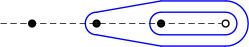
(a) $\ell_{E}$

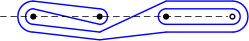
(b) $\sigma_{1}\sigma_{1}\cdot\ell_{E}$

Figure 1: Top: The loop $\ell_{E}$ for the $3$-punctured disk, used in the iterative computation of topological entropy (1). The three main punctures are black, while the white puncture serves as the “basepoint” for the loop. Bottom: $\ell_{E}$ after deformation by the braid $\sigma_{1}\sigma_{1}$, which exchanges the first pair of punctures twice, clockwise.

This iterative calculation may however be an inappropriate measure of complexity of trajectories. First, unless the trajectories correspond to periodic orbits, there is no justification for repeated application of the braid, since in that case the physical braid does not represent a homeomorphism of a fixed punctured surface. Second, flows that stretch material sub-exponentially will always be assigned $h(\mathbf{b})=0$, which may be too crude of a measure in practice, e.g., for estimating time-scales for transport.

Dynnikov and WiestDynnikov and Wiest (2007) used a non-iterated version of (1) to study the connection between algebraic and geometric properties of braids. We adapt their definition here to define the Finite-Time Braiding Exponent as a measure of complexity of trajectories.

Definition (Finite-Time Braiding Exponent).

Let $\mathbf{b}$ be a braid corresponding to $n$ trajectories over a time interval of length $T$. The Finite-Time Braiding Exponent is given by

$$\operatorname{FTBE}(\mathbf{b})=\frac{1}{T}\,\log\frac{\left\lvert{\mathbf{b}\ell_{E}}\right\rvert}{{\left\lvert{\ell_{E}}\right\rvert}}$$ (2)

where $\ell_{E}$ is the loop representing a generating set of the non-oriented fundamental group on $n$-punctured disk.

A similar definition of exponential deformation rate appeared in ref. Thiffeault, 2010, which uses an arbitrary loop $\ell$ instead of $\ell_{E}$.

III Constructing braids and computing FTBEs

Our ultimate goal is to use FTBEs as an approximation to topological entropy of a planar dynamical system. In this section we discuss the issues involved in constructing braids from data, introduce our model system, and examine the sensitivity of braids and FTBEs to various model parameters.

III.1 Practical considerations

To compute FTBEs, we must first construct braids. To do this, we record a finite number of concurrent, non-intersecting trajectories of the dynamics. Such a data set is determined by three parameters:

1. the number $n$ of trajectories,

2. the initial conditions of trajectories, and

3. the time interval $[t_{0},t_{0}+T]$ during which trajectories are recorded.

The MATLAB toolbox braidlab Thiffeault and Budišić (2014) converts trajectories into braids and then computes FTBEs. braidlab is an open-source library that implements a wide set of operations on braids, loops, and related structures. In particular, braids generated from data as discussed here are stored as databraid data structures, which record both crossings of strands as generators and the times at which crossings occurred.

The computational time to convert $n$ trajectories to a braid scales quadratically with $n$, and linearly with both the length of trajectories and the total number of crossings between strands. The algorithm depends on two additional parameters:

1. the angle $\alpha$ of the projection axis used to assign order to strands; and

2. the time step $\tau$ at which trajectories are sampled, assuming uniform sampling.

To accurately convert discretized trajectories to a braid, braidlab requires that strands cross only between sampled times, and that any two strands cross at most once per time step. If strands cross exactly at the moment of sampling, a braid generator cannot be unambiguously assigned. Such degeneracies may be resolved by varying the angle $\alpha$Thiffeault and Budišić (2014).

When two strands cross more than once in a single time step, other ambiguities can arise. For example, Figure 2 shows three different physical braids with same strand positions at the sampling time steps. The ambiguity can clearly be resolved by reducing $\tau$.

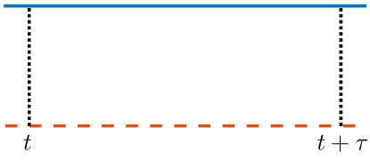
(a)  Identity (trivial) braid

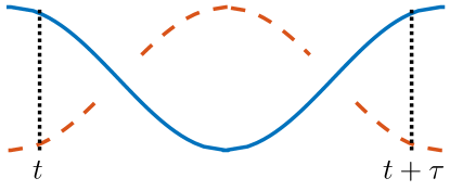
(b)  $\sigma_{i}\sigma_{i}^{-1}$ braid

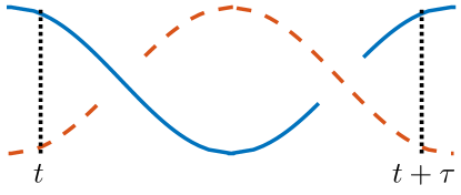
(c)  $\sigma_{i}\sigma_{i}$ braid

Figure 2: Three physical braids with same orders of strands $i$, $i+1$ at sampling times $t$ and $t+\tau$, but different sequences of generators. Using time step $\tau/2$ would resolve the crossings correctly.

The sections that follow demonstrate the dependence of FTBEs on each of the five parameters listed above: number of strands $n$, initial conditions, duration of time interval $T$, projection angle $\alpha$, and time step $\tau$. The input trajectories are generated by a mixing dynamical system, the Aref Blinking Vortex flow.

III.2 The Aref Blinking Vortex flow

The Aref Blinking Vortex flowAref (1984) is an idealization of a device that stirs fluid using two counter-rotating vortices in a circular domain. The vortices are otherwise identical, and are positioned along the diameter of the unit circle at distances $\pm b$ from its center. They are turned on alternately (“blinked”) during half of the period $T_{P}$ of the protocol, resulting in continuous, piecewise-differentiable trajectories of fluid parcels, shown in Figure 3. After fixing the geometry, and period of the protocol to $T_{P}=1$, the only free parameter is the non-dimensional circulation $\mu$. We restrict our analysis to $\mu\in[3,9]$ for which numerical experiments indicate that the flow is mixing in the entire domain.Aref (1984)

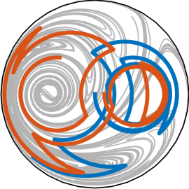
Figure 3: Material advection patterns and two particle trajectories of the Aref Blinking Vortex flow in the mixing regime.

We quantify the complexity of the flow by estimating topological entropy $h$ using direct advection of material curves Newhouse and Pignataro (1993). Numerically, we seed initial conditions along a randomly selected straight material line and advect those points forward. When distances between neighboring points grow too large, we linearly interpolate additional points between them to ensure that details of bends in the material curve are well represented.

Figure 4 shows the estimated values of topological entropy $h$ that will be used as reference for our later calculations of FTBEs. Topological entropy $h$ is approximately linear in circulation $\mu$, which determines the dominant time scale of the flow.

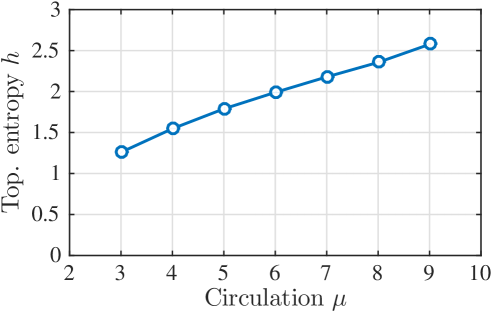
Figure 4: Topological entropy of counter-rotating Aref Blinking Vortex flow

III.3 Robustness of braid construction

In this section we investigate numerical issues involved in braid construction, which could lead to poorly-defined braids if not treated properly. The two main issues are the choice of time step (sampling rate, subsubsection III.3.1) and the choice of projection angle (subsubsection III.3.2).

III.3.1 Time step

Let us investigate how the choice of the sampling interval $\tau$ affects accuracy of constructed braids and their FTBEs. We will use the word length of braids as a proxy for the accuracy of constructed braids, as reducing $\tau$ increases the number of crossings in the braid.

Vortices in Aref Blinking Vortex flow are modeled by singularities which we slightly regularize to avoid infinite velocities. After regularization, time step $\tau_{\ast}=10^{-4}$ is sufficient to accurately sample trajectories of the flow in the studied regime of circulations. For each set of initial conditions we compute a braid $b_{\ast}$ with time step $\tau_{\ast}$, which serves as a reference, and additional braids $b_{\tau}$ with larger values of time step $\tau$. Figure 5 shows how the relative errors

$$\left\lvert{1-\frac{\operatorname{FTBE}(\mathbf{b}_{\tau})}{\operatorname{FTBE}(\mathbf{b}_{\ast})}}\right\rvert,\text{ and }\left\lvert{1-\frac{L(\mathbf{b}_{\tau})}{L(\mathbf{b}_{\ast})}}\right\rvert,$$ (3)

depend on time step $\tau$. To reduce the effect of spatial variations, we plot the largest relative errors with among different uniformly-initialized braids.

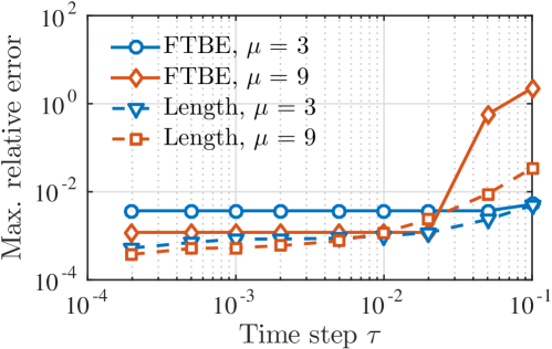
Figure 5: Effect of time step $\tau$ on relative error in FTBE and braid word length (3) with respect to the reference time step $\tau_{\ast}=10^{-4}$. Graph shows the maximum error among $100$ braids of 50 uniformly initialized strands.

Figure 5 suggests that FTBEs are more resilient to large time steps than word length. This implies that some parts of the braid do not contribute significantly to deformation of loops. For example, a braid of four generators $\sigma_{i}\sigma_{i}^{-1}\sigma_{i}\sigma_{i}^{-1}$ introduces no net deformation as each inverse generator reverses the action of the previous one. Such sequences can be generated by pairs of strands that are neighbors along the projection line, but are otherwise located far from each other in the domain.

As expected, the effect of large time steps is more pronounced for flows with larger circulations $\mu$, as particles move farther within each time step. We use $\tau=10^{-2}$ for the rest of the paper, which is appropriate for our range of $\mu$.

III.3.2 Angle of the projection axis

The angle $\alpha$ determines the projection line used to assign order indices to strands of a physical braid. As mentioned at the opening of Section III, $\alpha$ may need to be adjusted to ensure that trajectories can be converted to a braid. We show that even though the braid itself changes depending on $\alpha$, the effect on FTBEs is minimal.

When a physical braid consists of periodic trajectories, changing $\alpha$ results in conjugation of the corresponding braid $\mathbf{b}$ by another braid $\mathbf{c}_{\alpha}$. In other words, dependence on angle $\alpha$ enters into the braid as $\mathbf{c}_{\alpha}^{-1}\mathbf{b}\mathbf{c}_{\alpha}$. However, when strands in the physical braid are not periodic, changing $\alpha$ is not guaranteed to affect the braid through conjugation only Thiffeault and Budišić (2014). Nevertheless, since changing $\alpha$ only rotates the coordinate system, the FTBEs should not significantly depend on $\alpha$.

Figure 6 shows how length $T$ of trajectories influences statistics of FTBEs and braid word length with respect to projection angle $\alpha$. It is clear that the change of projection angle minimally affects the value of FTBEs for longer braids. Over the entire range of times $T$ simulated, the Relative Standard Deviation (RSD) of FTBEs decays inverse-proportionally with length of the physical braids, while the standard deviation of length remains approximately constant, indicating that FTBEs are more robust than braid length with respect to change of $\alpha$. Based on this, we set $\alpha=0$ in the remainder of this paper.

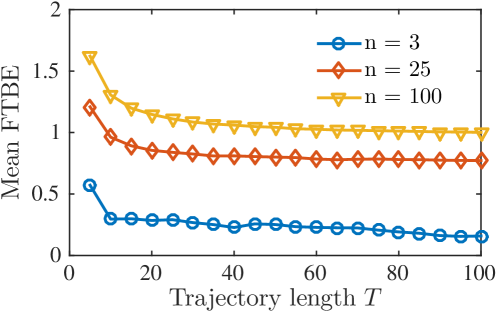
(a)  Mean FTBE

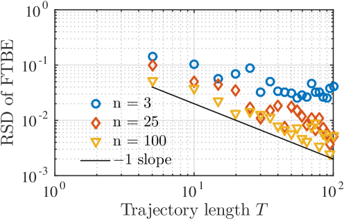
(b)  Relative Standard Deviation of FTBE

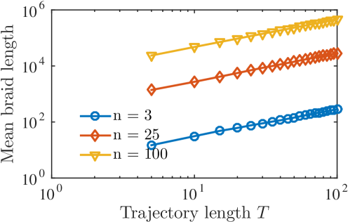
(c)  Mean braid word length

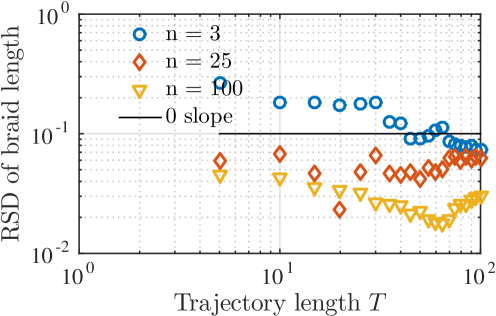
(d)  Relative Standard Deviation of braid word length

Figure 6: Effect of projection angle $\alpha$ on FTBEs and braid word length of a single physical braid. Statistics are computed with respect to uniform distribution of $100$ angles $\alpha\in[0,\pi)$. Circulation is $\mu=5$.

III.4 Parameters for braid construction

In subsection III.3 we addressed numerical issues that can lead to deviations from the idealized mathematical representation of braids. In this section we turn to parameters that affect the nature of the braid we obtain. These are the choice of initial conditions, the length (duration) of trajectories (subsubsection III.4.1), and the number of trajectories (subsubsection III.4.2).

III.4.1 Initial conditions and length of trajectories

FTBEs can be interpreted as measures of average deformation of a loop over finite segments of physical braids. Averaged measurements in chaotic systems quickly stabilize to constant values independent of precise initial conditions, which is formally asserted by various flavors of ergodic theorems. Since numerical evidence indicates that the Aref Blinking Vortex flow is mixing for $\mu\in[3,9]$, the FTBEs should not depend on initial conditions for long-enough trajectories.

Figure 7 confirms the expected ergodic behavior. After the rapid initial transient, the spatial mean of FTBEs settles to a constant value, while spatial fluctuations decay following a power law. Since the length of the transient does not depend on number $n$ of strands, we set the length of trajectory to $T=100$ in future simulations.

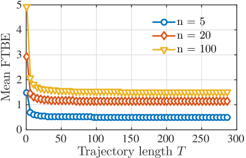
(a)  Mean FTBE

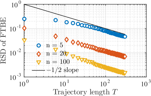
(b)  Relative Standard Deviation of FTBE

Figure 7: Effect of trajectory length $T$ on FTBE for an ensemble of physical braids. Statistics are computed with respect to uniform initialization of 100 physical braids. The circulation is $\mu=5$.

The slope $-1/2$ of decay of fluctuations is commonly associated with the Central Limit Theorem for sums of random variables. Variants of the Central Limit Theorem apply to the decay in fluctuations of Finite-Time Lyapunov Exponents in mixing flows Hennion (1997); Young (1998). While we provide no rigorous proof that the same applies to FTBEs, it is not surprising to see the same behavior since FTBEs and FTLEs are closely-related quantities.

III.4.2 Number of strands

It has been observed that using more trajectories increases the complexity of the braid Finn and Thiffeault (2007); Thiffeault (2005); Tumasz (2012). To study how FTBEs depend on the number of strands $n$, we fix the length of trajectories to $T=100$ and at each value $n$ compute mean and standard deviation of the FTBE with respect to initial conditions.

Figure 8 shows that mean $\operatorname{FTBE}$ and mean braid word length grow in a different manner with addition of strands. The mean $\operatorname{FTBE}$ appears to limit to topological entropy $h$; on the other hand, the number of crossings $L$ is unbounded, growing proportionally to the number of pairs of strands $n^{2}$. The standard deviations of both FTBE and word length decay according to a power law, although with slightly different slopes.

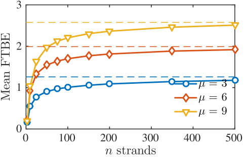
(a)  Mean FTBE. Horizontal lines indicate topological entropies $h$.

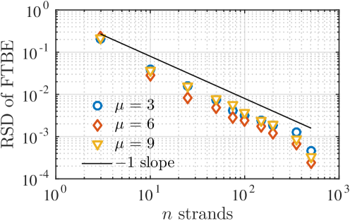
(b)  Relative Standard Deviation of FTBE

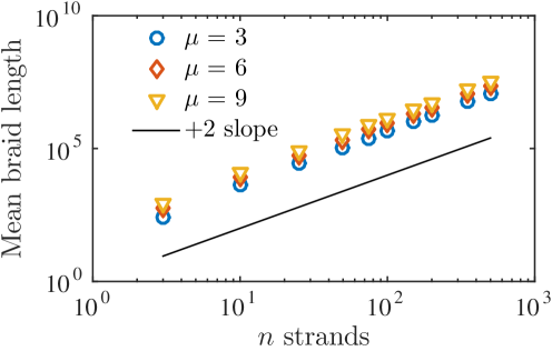
(c)  Mean braid length

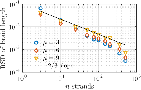
(d)  Relative Standard Deviation of braid length

Figure 8: Influence of number $n$ of strands on FTBE and length of an ensemble of physical braids. Statistics are computed with respect to uniform initialization of 100 physical braids.

To generate Figure 8 we computed approximately $S\times\sum_{\mathrm{points}}n\approx 150,000$ trajectories of the Aref Blinking Vortex flow. While such a large number of trajectories can be computed for numerical flows, the number of trajectories available experimentally is often much smaller, especially in systems featuring human crowds, flocks of birds, or oceanic floats. We can, however, generate collections of braids by re-using data from a much smaller set of trajectories.

If we have access to $m$ measured trajectories, we can form a single $m$-stranded braid, but also select subsets of $n<m$ trajectories to form smaller $n$-subbraids. There are ${m\choose n}$ different $n$-stranded subbraids, which is a number that grows fast as $n\to m/2$ from above or below. Therefore, it is easy to obtain large collections of $n$-braids by selectively including strands of a bigger set of $m$ trajectories.

Despite the practical appeal, it is not clear that statistics of FTBEs and braid lengths will be similar if calculated using either independent braids or subbraids of a larger braid; subbraids are not mutually independent, as they re-use the same set of trajectories from the original data set. To compare statistics, we generate subbraids from a single set of $m=550$ trajectories for the same values of $n$ used in the calculations Figure 8, which used independent sampling. Figure 9 overlays the results of two calculations and indicates that statistics of FTBEs over subbraids match almost perfectly with statistics over independently sampled braids.

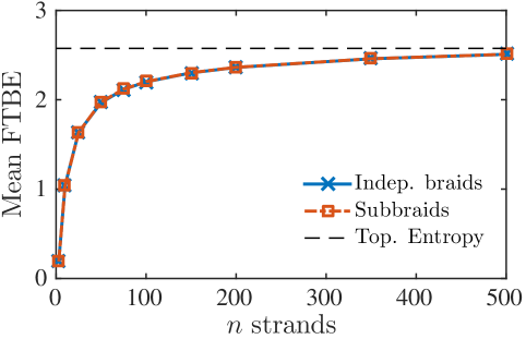
(a)  Mean FTBE

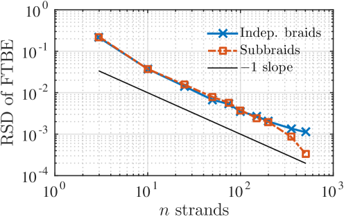
(b)  Relative Standard Deviation of FTBE

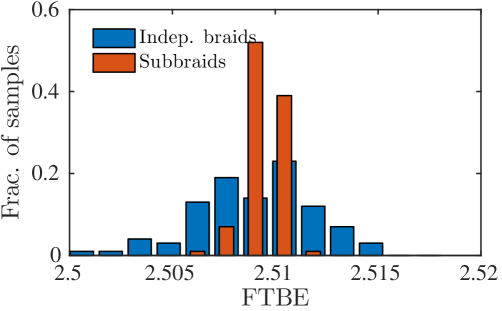
(c)  Distribution of FTBE at $n=500$, value with largest difference in RSD between two sets.

Figure 9: Comparison of FTBE for braids sampled independently and braids formed as subbraids of $m$ strands chosen from a single $m=550$ braid. Sample size at every parameter value is $S=100$, circulation $\mu=9$.

An additional practical benefit of using subbraids is the speed of generating them. The time to extract one $n$-subbraid from a full $m$-braid scales with the braid word length of the full braid. This procedure is generally much faster than forming an independent $n$-braid, even if the time to simulate new trajectories is negligible. In our example statistics over subbraids were computed $5$ to $10$ times faster than over independent braids.

IV Extrapolating topological entropy from FTBEs

Figure 10 demonstrates that topological entropy $h$ of the flow and mean values of FTBEs are strongly correlated, therefore the FTBE can serve as a finite-scale proxy for $h$. To go further, and extrapolate values of FTBE to obtain the actual value of topological entropy $h$, we need that: 1) the FTBE indeed approaches topological entropy as $n\to\infty$, and 2) the growth of $\operatorname{FTBE}$ can be described by a relatively simple functional model, whose parameters can be estimated. Neither of these statements are rigorously known to be true. Previous numerical results indicate that topological entropy of braids formed by periodic trajectories approaches the topological entropy of the flow, but there are no formal verifications Finn and Thiffeault (2007). The results of Section III.4.2 suggest that FTBEs behave similarly.

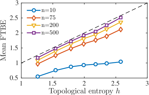
Figure 10: Correlation of topological entropy and mean FTBEs computed using different numbers of strands $n$. Points were obtained by varying circulation $\mu$.

To investigate the approach of FTBEs to topological entropy $h$, we compute the relative difference $1-\operatorname{FTBE}/h$, and compute its statistics across sets of $S=100$ subbraids of a physical braid of $m=550$ trajectories. Figure 11 shows that the relative difference approximately decays as a power law with slope $-1/2$ for a large range of strands $n$. Nevertheless, the decay deviates from the power law as $n$ increases, which means that extrapolating data using a power law model would overestimate the value of topological entropy.

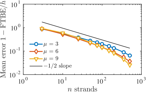
Figure 11: Relative difference of the mean FTBE and topological entropy $h$ for the Aref Blinking Vortex flow. Statistics are computed with respect to $100$ $n$-subbraids of a set of 550 trajectories of length $T=100$.

To estimate the decay of the relative difference more carefully, we fit two functions to the calculated points:

Tempered Power Law

$$n^{\gamma}e^{\beta n}$$ (4)

Log-normal CDF

$$\operatorname{erfc}\{\gamma\log\beta n\}$$ (5)

These two functions are often used as competing statistical models for tails of distributions, where the criterion for choosing one over the other is based on a maximum likelihood estimation. Clauset, Shalizi, and Newman (2009); Mitzenmacher (2004) Since relative difference at $n$ strands is not associated with a distribution, we use the more classical weighted least-squared-error fitting of models to data. Weights assigned to data points are inversely proportional to the standard deviation of FTBEs, which enforces a tighter fit to points at larger $n$, due to decaying standard deviation, shown in Figure 9(b).

Figure 12 shows the quality of fit of the two models to values of FTBEs. Both functions fit well to data, as evidenced by Figure 12(a). Figure 12(b) shows residual errors for both models at different values of circulation and demonstrates that the tempered power law fits slightly better.

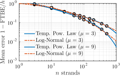
(a)  Fit of functions  (4) and (5) (lines) and data (circles) to relative difference between mean FTBE and topological entropy

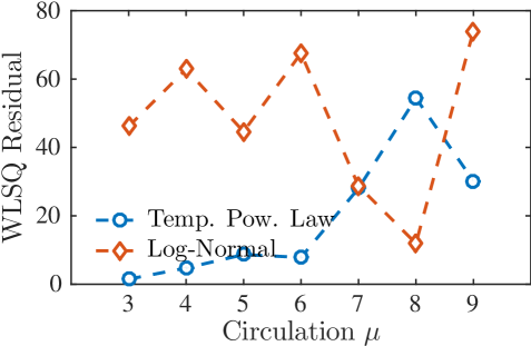
(b)  Weighted least-squared-error fit residuals

Figure 12: Quality of fit of Tempered Power Law and Log-normal CDF models to computed mean FTBE

The true test of the models should be their ability to correctly predict the topological entropy $h$ as their limit. Instead of using values of $h$ as a known limit of proposed models, we introduce a limit parameter $h_{\infty}$ and allow it to vary during fitting. This additionally means that we fit our model functions to FTBE data instead of the relative difference to a reference value. Other than these modifications, models and fitting technique remain the same.

Unsurprisingly, we again find that both models provide a tight fit to data; however, their limits differ due to different rates of growth as $n\to\infty$. Figure 13 shows relative differences $1-h_{\infty}/h$ between extrapolated limits of FTBE $h_{\infty}$ and topological entropy $h$, depending on circulation $\mu$. In addition to fitting models to all available data points, we also fit them to data sets with points at higher values of $n$ removed, to test robustness of the extrapolations $h_{\infty}$ to the amount of data used. Only non-negative values of differences are consistent with the expectation that values of FTBE approach $h$ from below as $n\to\infty$.

Figure 13 demonstrates that the Log-normal model consistently overestimates the value of topological entropy. On the other hand, extrapolations of the tempered power law provide a better estimate than the raw FTBE calculation at the largest number of strands (in blue), while remaining consistent with the theory. We note that extrapolating the fit up to $m=350$ strands yields an estimate that is of similar quality to estimation of $h$ by FTBE at $n=500$ strands without extrapolation. This translates to savings in data collection and analysis time, since converting trajectories to braids takes $\mathcal{O}(n^{2})$ time to complete, and computing a single braid at a large $n$ can take longer than computing many collections of subbraids at $m<n$.

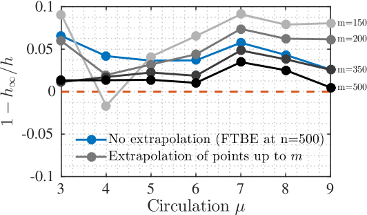
(a)  Tempered Power Law

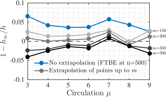
(b)  Log Normal CDF

Figure 13: Comparison of $h_{\infty}$ obtained by extrapolating tempered power law and log-normal models for mean FTBE. Blue lines show the best estimate of topological entropy obtained without extrapolation. Different gray lines connect values $h_{\infty}$ obtained from models fit to larger and larger point sets; number next to the line is the number of strands of last point used for fitting.

The numerical evidence indicates that a tempered power law models the approach of FTBE to topological entropy, with power law exponents $\gamma$ estimated to lie in $[-0.4,-0.5]$. Fixing the exponent of the tempered power law to $\gamma=-1/2$ minimally changes quality of fit and extrapolation by the tempered power law model, suggesting that growth of FTBE follows an universal behavior, regardless of circulation of the flow.

We caution, however, against making stronger arguments based on the experiments performed, because the reference value for topological entropy $h$ is an estimate itself, computed by material advection. Since the precision achieved by FTBE is within 1% to 5% of $h$, it is likely that it approaches the confidence interval for the estimation by material advection. For quantitative conclusions about the approach of FTBE to topological entropy of the flow, analytical justification for a model of growth of FTBE is needed.

V Discussion

We briefly summarize our findings about Finite-Time Braiding Exponents.

• FTBEs are very robust with respect to the projection angle $\alpha$ used to construct the braids.

• Reasonably-small values of the time step $\tau$ lead to well-defined braids, but FTBEs may tolerate a larger $\tau$.

• Increasing the length of trajectories in mixing dynamics results in convergence of FTBEs. At the same time, the spatial mean of FTBEs stabilizes, while their spatial fluctuations decay.

• The spatial mean of FTBEs correlates strongly with the topological entropy of the flow; as the number of strands $n$ is increased, the mean approaches the topological entropy.

The Finite-Time Braiding Exponent of $n$ trajectories sampled from the flow can be interpreted as a “multi-scale” measure of complexity of the flow at scales determined by $n$. An important finding is that to estimate complexity at different scales, a single collection of $n$ trajectories can be re-used by sampling subbraids. Even though such subbraids are not fully independent, since a given trajectory will participate in many braids, the procedure yields statistics of FTBEs similar in quality to those computed using independently-sampled braids. This technique greatly reduces the required amount of input data without sacrificing the quality of computed FTBEs at various scales.

The value of FTBEs seems to approach the topological entropy of the flow as $n$ is increased, but more work is needed to establish the asymptotics of that approach. Fitting plausible functional models suggests that for trajectories of mixing dynamical systems the difference between FTBEs and topological entropy decays according to a power law tempered by an exponential. If confirmed analytically, this relation would allow one to estimate free parameters of the model from values of FTBEs at several different scales $n$, and extrapolate the model as $n\to\infty$ to approximate the topological entropy very closely.

While these conclusions are based on the study of the Aref Blinking Vortex flow, it is reasonable to expect similar results for other mixing flows. In flows that are not spatially homogeneous, e.g., those containing coherent substructures, lengths of strands and locations of their initial conditions will be of crucial importance for interpretation of FTBE values. In such situations, other quantities based on braids can be computed to provide a more complete picture of dynamics. In particular, a promising approach may be to couple braid approximations of coherent structuresAllshouse and Thiffeault (2012) with FTBE estimates of complexity inside those structures to assess the spatial distribution of different dynamics in more complicated flows, even when the only information available is a finite set of trajectories.