Chemical Abundances in the Globular Clusters NGC 6229 and NGC 6779

Abstract

Long-slit medium-resolution spectra of the Galactic globular clusters (GCs) NGC 6229 and NGC 6779, obtained with the CARELEC spectrograph at the 1.93-m telescope of the Haute-Provence observatory, have been used to determine the age, helium abundance (Y), and metallicity [Fe/H] as well as the first estimate of the abundances of C, N, O, Mg, Ca, Ti, and Cr for these objects. We solved this task by comparing the observed spectra and the integrated synthetic spectra, calculated with the use of the stellar atmosphere models with the parameters preset for the stars from these clusters. The model mass estimates, $T_{\rm eff}$, and $\log\leavevmode\nobreak\ g$ were derived by comparing the observed ‘‘color–magnitude’’ diagrams and the theoretical isochrones. The summing-up of the synthetic blanketed stellar spectra was conducted according to the Chabrier mass function. To test the accuracy of the results, we estimated the chemical abundances, [Fe/H], $\log\leavevmode\nobreak\ t$, and $Y$ for the NGC 5904 and NGC 6254 clusters, which, according to the literature, are considered to be the closest analogues of the two GCs of our study. Using the medium-resolution spectra from the library of Schiavon et al., we obtained for these two clusters a satisfactory agreement with the reported estimates for all the parameters within the errors. We derived the following cluster parameters. NGC 6229: $[Fe/H]=-1.65$ dex, $t=12.6$ Gyr, $Y=0.26$, $[\alpha/Fe]=0.28$ dex; NGC 6779: $[Fe/H]=-1.9$ dex, $t=12.6$ Gyr, $Y=0.23$, $[\alpha/Fe]=0.08$ dex; NGC 5904: $[Fe/H]=-1.6$ dex, $t=12.6$ Gyr, $Y=0.30$, $[\alpha/Fe]=0.35$ dex; NGC 6254: $[Fe/H]=-1.52$ dex, $t=11.2$ Gyr, $Y=0.30$, $[\alpha/Fe]=0.025$ dex. The value $[\alpha/Fe]$ denotes the average of the Ca and Mg abundances.

1 INTRODUCTION

There are about 150 globular clusters (GCs) in our Galaxy with different luminosities, sizes, and stellar density in the center harris96:Khamidullina_n . The majority of GCs are old ($t=7$–$15$ Gyr). The clusters move with different velocities, at different distances relative to the Galactic center, and have different abundances. Objects with relatively high metallicity occur closer to the Galactic center. They are called bulge clusters. The GCs with the lowest metallicity ($-2.4<[Fe/H]<-1.5$ dex) occur in the halo of our Galaxy. The most distant of these objects is NGC 2419. Its galactocentric distance is equal to $R_{\rm GC}=84$ kpc which is 3.5 times greater than the distance $R_{\rm GC}=24$ kpc of the nearest dwarf spheroidal to the Milky Way: the Sagittarius dSph. The typical parameters of GC subsystems and their population characteristics are described, e.g., in Borkova and Marsakov mars:Khamidullina_n .

The metallicities of the majority of GCs are derived from a comparison of stellar photometry results and theoretical evolutionary tracks and isochrones. The brightest cluster stars are investigated with high resolution spectrographs. By no means all of the Galactic GCs have been studied spectroscopically. The clusters of our study (NGC 6229 and NGC 6779 (M 59)) belong to such poorly studied objects.

Table 1: The key parameters of the studied and comparison globular clusters according to harris96:Khamidullina_n : heliocentric distance ${\rm Dist}_{\odot}$; Galactocentric distance ${\rm Dist}_{\rm GC}$, assuming ${\rm Dist}_{\rm GC}=8$ kpc for the Sun; absolute $V$-band magnitude in the Johnson–Cousins photometric system; central $V$-band surface brightness; color excess; tidal radius $r_{t}$; core radius $r_{c}$; central concentration $c=\log(r_{t}/r_{c})$; central luminosity density logarithm

Parameter	NGC 6229	NGC 6779	NGC 5904	NGC 6254
${\rm Dist}_{\odot}$, kpc	$30.4$	$10.1$	$7.5$	$4.4$
${\rm Dist}_{\rm GC}$, kpc	$29.7$	$6.2$	$9.7$	$4.6$
$M_{V}$, mag	$-8.05$	$-7.38$	$-8.81$	$-7.48$
$\mu_{V}$, mag arcsec-2	$16.99$	$18.06$	$16.05$	$17.69$
$E(B-V)$, mag	$0.01$	$0.20$	$0.03$	$0.28$
$r_{t}$, pc	$47.6$	$25.15$	$61.96$	$27.49$
$r_{c}$, pc	$1.15$	$1.08$	$0.91$	$1.10$
$c$	$1.61$	$1.37$	$1.83$	$1.40$
$\log L_{\rm cent}$, $L_{\odot}/pc^{3}$	$3.41$	$3.26$	$3.91$	$3.5$

The basic properties of the studied objects are presented in Table 1 along with the parameters of the objects we chose from harris96:Khamidullina_n ; these two objects, NGC 5904 (M 5) and NGC 6254 (M 10), are their close analogues in terms of metallicity, age, horizontal branch type, and other parameters. We took the spectra of these GCs from Schiavon et al. schiavon:Khamidullina_n . All four GCs under consideration are massive, dynamically evolved objects with high stellar density in the center.

NGC 6229 is one of the most distant GCs of the outer halo. The photometry was performed and the ‘‘color–magnitude’’ diagram ($C$–$M$) was plotted for this cluster by several authors during 1986–1991 (see references in borissova97:Khamidullina_n ). The first deep photometry of the cluster core and periphery, including the full horizontal branch (HB) and the asymptotic giant branch, was performed by Borissova et al. with the 2-m telescope at NAO Rozhen, Bulgaria borissova97:Khamidullina_n ; borissova99:Khamidullina_n ; borissova01:Khamidullina_n . In these papers and also in catellan98:Khamidullina_n , the HB structure and the variable stars in NGC 6229 were investigated; the position of the main sequence (MS) turnoff point was also determined. Borissova et al. borissova99:Khamidullina_n were the first to note the similarity in the metallicity and age of NGC 6229 and NGC 5904. A common property of these two clusters is the presence of a considerable number of RR Lyrae-type variable stars. The blue stars brighter than the MS turnoff point (blue stragglers) were studied in sanna12:Khamidullina_n based on the Hubble Space Telescope images.

NGC 6779 is a low-metallicity globular cluster of the halo. It is comparatively poorly studied because of its close proximity to the Galactic plane. Hatzidimitriou et al. hatzidimitriou:Khamidullina_n presented a deep ground-based photometry of this cluster, and Sarajedini et al. sarajedini:Khamidullina_n and Dotter et al. dotter10:Khamidullina_n performed the stellar photometry based on the Hubble images. The authors estimated the metallicity and age of the cluster using the Dartmouth isochrones dartmouth:Khamidullina_n . Unlike NGC 6229, NGC 6779 has a low metallicity (see Table 1) and an extended blue horizontal branch.

NGC 5904 is the closest GC to us that is located far from the Galactic plane. That is why it is an excellent object for studying the abundances of individual GC stars, and for plotting deep $C$–$M$ diagrams. Its exact photometry serves for testing the stellar evolution models. The cluster includes a large number of variable stars. It has an enormous space velocity and a very eccentric orbit cud:Khamidullina_n . Two millisecond pulsars have been found in it, one of which is associated with a massive neutron star freire:Khamidullina_n . The nature of these objects is not clear yet. Coppola et al. coppola:Khamidullina_n estimated the distance to the cluster by the ‘‘period–infrared magnitude’’ relation for the RR Lyr-type stars: $(M-m)_{0}=14.44\pm 0.02$. Similar distance estimates were obtained by approximating the evolutionary sequences of the cluster with theoretical tracks using the Hubble photometry layden:Khamidullina_n ; vandenberg:Khamidullina_n .

NGC 6254 is one of the nearby clusters of the Galactic halo for which deep Hubble photometry is available. In particular, the photometry results allow one to determine the percentage of binaries as a function of distance to the center of NGC 6254 beccari:Khamidullina_n . This, in turn, made it possible to explain the low level of mass segregation in the cluster without invoking the hypothesis of an intermediate-mass black hole in the cluster center dalessandro:Khamidullina_n . The deep photometry performed on Hubble images and estimates of the distance and Galactic absorption for NGC 6254 were also presented in sarajedini:Khamidullina_n .

The integrated spectra of the two nearby clusters, NGC 5904 and NGC 6254, were included in the spectral library of Schiavon et al. schiavon:Khamidullina_n , which was used by different authors for numerous studies afterwards. The deep $C$–$M$ diagrams for the clusters NGC 6779, NGC 5904, and NGC 6254 layden:Khamidullina_n ; sarajedini:Khamidullina_n were widely used for the investigation of the cluster evolutionary status and testing the stellar population models. VandenBerg et al. VRmodel:Khamidullina_n determined the age, [Fe/H], and helium abundance index for NGC 6779, NGC 590, and NGC 6254 applying their Victoria-Regina models.

Nowadays, with the development of observational and computing techniques for the analysis of the individual stars in GCs and also for the determination of their parameters, the method of synthetic spectra, calculated using stellar model atmospheres, is often used. By varying the abundances of different chemical elements, the deviation of the theoretical spectra from the observed ones is minimized. The used spectral range should be large enough to include both a sufficient number of lines of the same element with different degrees of ionization and numerous lines of various elements. To obtain the fullest and most accurate data, one should obviously use spectra with the highest possible resolution. However, obtaining such spectra with a sufficiently high $S/N$ ratio requires much observing time with large telescopes, and is possible only for the brightest stars. The analysis of the integrated light of the clusters allows us to efficiently process the data obtained with 1–2-m telescopes for all the objects in the Galaxy, and the data from large telescopes—for extragalactic clusters. This approach is adopted in this paper for the four above-mentioned clusters. It allowed us to obtain valuable data for the comparison of the photometric and spectral stellar evolution models which is the essential basis for understanding the properties of the stellar populations in other galaxies.

In Section 2 the observations and their reduction techniques are described. In Section 3 we present the method of modeling the integrated cluster spectra in accordance with the data on the isochrones and the luminosity function, and of determining the chemical abundances. In Section 4 the results of the investigation are discussed, and the conclusions are formulated in Section 5.

2 OBSERVATIONS AND REDUCTION

We have observed the clusters NGC 6229 and NGC 6779 with the 1.93-m telescope of the Haute-Provence observatory for a comparative analysis of their stellar populations and the characteristics derived from the study of the $C$–$M$ diagrams. The observation log is presented in Table 2. Long-slit medium- resolution spectra ($5.5^{\prime}\times 2^{\prime\prime}$) were obtained with the CARELEC coppola:Khamidullina_n spectrograph. We used a 300 lines/mm grating, which provided a dispersion of about $1.78$ Å per pixel and a $\sim 5$ Å(FWHM) spectral resolution in the working spectral range of $3700$–$6800$ Å. Calibration exposures with HeNe lamps were taken at the beginning and end of each night. The observations were carried out in adverse weather conditions with cirrus and intermittent clouds. The average seeing was $2.5$–$3.5$". However, the lack of illumination from the moon allowed us to obtain the CCD images of required quality during clear sky periods. Table 2 shows that the observations were carried out with several fixed slit positions. In all cases the slit was oriented so as to capture not only the central, brightest part of a GC but also the neighboring regions highly populated with stars. Thus, the resulting 2D image permitted us to compare the energy distributions and individual spectral lines of the central region, unresolved into individual objects, and the neighboring stars. As a result, we could safely eliminate the background objects that could distort the GC abundances from the one-dimensional sum spectrum. Note that other authors usually use a scanning technique with a moving slit to obtain the integrated GC spectrum (see, e.g., schiavon:Khamidullina_n ). This technique enhances the probability of background objects entering into the resulting spectrum, especially in the case of GCs close to the Galactic plane.

Table 2: Log of spectroscopic observations

Object	Date	Exposure,	Slit
		s	position, deg.
NGC 6229	09.07.10	600	0
		600	90
NGC 6779	09.07.10	300	95
		300	99
	11.07.10	2 $\times$ 900	0

Primary data reduction was conducted using MIDAS midas:Khamidullina_n and IRAF software packages. First, we filtered out cosmic ray hits with the filter/cosmic code in MIDAS environment. Hot pixels were masked. The standard procedure of spectra reduction was then conducted: bias substraction, flat-field correction. The dispersion relation provided an accuracy of wavelength calibration of about $0.8$ Å. One-dimensional spectra were extracted with the IRAF apsum procedure. The final signal-to-noise ratio per pixel at the center of the spectral range of the obtained spectra was $S/N\approx 130$. The continuum in the one-dimensional spectra was approximated with the MIDAS filter/maximum and filter/smooth (running median) functions. The analysis of the correspondence of the observed and theoretical spectra was conducted in the Origin 6.1 graphical environment.

3 METHOD OF DETERMINATION OF THE CHEMICAL ABUNDANCES AND EVOLUTIONARY PARAMETERS OF GLOBULAR CLUSTERS

The method used in this paper was first presented by Sharina et al. sharina:Khamidullina_n . The method applies not only to spectral but also to photometric observational and theoretical data. It is based on a comparison of the observed GC spectra and model spectra derived by summing up the individual synthetic spectra of stars with different masses, $\log\leavevmode\nobreak\ g$, and $T_{\rm eff}$. The stellar parameters are set by the isochrone best corresponding to the cluster $C$–$M$ diagram. The method for estimating the abundances and evolutionary parameters described in this section can be applied to any globular cluster for which deep stellar photometry and a long-slit spectrum containing the information on all the stars of the cluster are available. The spectra of the dense central GC regions are best suited for such an analysis. Our method is applicable to spectra with a resolution of $R>2500$, a rather high signal-to-noise ratio ($S/N>100$), and a spectral range of no less than $1500$ Å.

3.1 Determination of Masses, $\log\leavevmode\nobreak\ g$, and $T_{\rm eff}$
for Cluster Stars

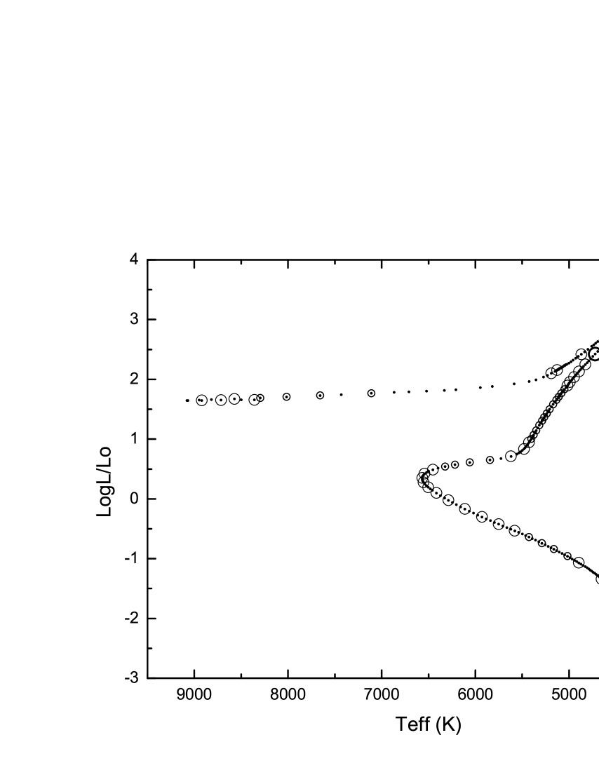
5mm normal

Figure 1: The isochrone $\log\leavevmode\nobreak\ t=10.1$, $Y=0.26$, $Z=0.0004$ for NGC 6229. The circles of different sizes denote the points (in the circle centers) which contribute less than 1%, from 1% to 3%, and more than 3% to the total flux.

The synthetic blanketed spectra of stellar atmospheres are calculated according to the physical stellar parameters derived from the comparison of the observed $C$–$M$ diagrams of the clusters and the theoretical isochrones from Bertelli et al. bert1:Khamidullina_n . For our work we chose the isochrones obtained by the Padova team. This choice was determined by the fact that the authors included the evolutionary stages of the HB and the asymptotic giant branch in the models and also used a wide range of parameters: metallicity [Fe/H], age $t$, and helium abundance $Y$. For the clusters NGC 6229 and NGC 6779 we used the stellar photometry data from Piotto et al. piotto:Khamidullina_n and Sarajedini et al. sarajedini:Khamidullina_n .

When selecting a theoretical isochrone which best fits the cluster $C$–$M$ diagram, we vary five parameters: age $t$, specific helium abundance $Y$, metallicity [Fe/H], color excess $E(B-V)$, and distance to the cluster. As initial parameters, we used data from the following references: Harris’s compiled catalog harris96:Khamidullina_n and Vandenberg et al. vandenberg:Khamidullina_n , who determined the parameters based on stellar photometry of Sarajedini et al. sarajedini:Khamidullina_n and Victoria-Regina VRmodel:Khamidullina_n models. The initial metallicities and ages for a number of clusters were adopted from Dotter et al. dotter10:Khamidullina_n , whose results were derived with the use of isochrones from Dartmouth dartmouth:Khamidullina_n .

Isochrone selection is carried out in the following way.

• (1) The position of the basic evolutionary sequences: main branch, subgiant branch, red giant branch, and horizontal branch, is computed from the photometric data as a running median with a step of $0.1$’ along two coordinates (color and magnitude). Stars with magnitude measurement errors larger than $0.2$’ should previously have been excluded from the photometry table. Those are the faint objects. Usually, the percentage of their detection on Hubble images does not exceed 50$\%$. Consequently, the fiducial sequence of the $C$–$M$ diagram is plotted, which describes the position of the basic evolutionary sequences of a cluster.

• (2) Next, the theoretical isochrone minimally deviating from the fiducial sequence is selected. This is done by $\chi$-square minimization:

  $$\chi^{2}=\displaystyle\sum_{i=1}^{N}\left[\displaystyle\frac{I_{o}-I_{m}}{\sigma_{I_{o}}}\right],$$

  where$I_{o}$, $\sigma_{I_{o}}$ are the magnitudes of the fiducial and their errors, and $I_{m}$ are the corresponding isochrone values. Note that we do not interpret theoretical isochrones but merely use the available set bert1:Khamidullina_n .

Variations of the Galactic absorption in the direction of a GC and the distance to a cluster do not influence the inclination, form, and relative position of different evolutionary sequences, but shift the $C$–$M$ diagram as a whole. Variations of [Fe/H], $t$, or $Y$, on the other hand, influence the position and form of the isochrones (see, e.g., the explanation in bert1:Khamidullina_n ). The evaluation of the basic evolutionary parameters from the $C$–$M$ diagram is conducted taking into account these variations. In the following six paragraphs, we explain the principles of determining [Fe/H], $t$, and $Y$.

Selection of [Fe/H] ($t$, $Y$ are constant) is performed by the inclination of the red giant branch salaris02:Khamidullina_n as the basic criterion. The inclination of the branch increases with the increase of [Fe/H], and the luminosity of the stars at the top of the red giant branch falls more and more rapidly at $[Fe/H]\geq-0.8$ dex. Moreover, with increasing metallicity, the whole isochrone shifts toward the red region, the luminosity of the stars in it decreases, and fewer hot blue stars appear on the HB.

Selection of the age value ([Fe/H] and $Y$ are constant) is done using the temperature and luminosity of the MS turnoff stars. With increasing age, the MS turnoff point position shifts toward cooler and fainter stars and is additionally dependent on the GC chemical abundance. The luminosity of HB stars is mainly determined by metallicity and helium abundance. There are two basic and common empirical approaches to relative age estimation for GCs: a vertical one iben71:Khamidullina_n ; iben91:Khamidullina_n ; VDBerg90v:Khamidullina_n , which takes into account the difference in the luminosities of the MS turnoff point and the zero age HB ($\delta V=V_{\rm TO}-V_{\rm ZAHB}$), and a horizontal one VDBerg90g:Khamidullina_n , based on the difference in temperature (color) between the MS turnoff point and the base of the red giant branch $\delta(B-V)=(B-V)_{\rm RGB}-(B-V)_{\rm TO}$.

In iben91:Khamidullina_n , an approximate ratio between $\delta V$, the abundances of helium $Y$ and heavy elements $Z$ on the one hand, and the logarithm of age on the other hand is given. As a consequence of the strong dependence of the HB star luminosities on $Y$, and the MS turnoff point on $Z$, the vertical method provides only the relative ages for GCs of similar metallicity and $Y$. For the estimation of absolute ages, the exact values of the helium mass fraction are needed.

The essence of the horizontal method is in measuring the color difference between the MS turnoff point, sensitive to age, and the red giant branch, sensitive to metallicity. This method is also relative. The compared clusters should have the same metallicities and $[\alpha/Fe]$.

It is necessary to note that both the vertical and horizontal methods do not require knowledge of absolute distances to the observed objects and of the light absorption in their direction. There are numerous modifications of these two approaches (see, e.g., carney:Khamidullina_n ; roediger:Khamidullina_n . The results of age estimation for the same cluster using different methods vary greatly. Modern researchers use a maximum likelihood method for isochrone selection for the $C$–$M$ diagram of a cluster as a whole. We use a similar method. Estimation of the MS turnoff point magnitude is rather difficult and often leads to an age inaccuracy of about 10%. That is why the approximation by an isochrone of the $C$–$M$ diagram as a whole with all its bends is much more precise. As we use not only the photometric data characterizing the stellar luminosities and temperatures but also spectroscopic data on the detailed abundances, further development of our method could allow us to estimate the absolute ages of the clusters.

Variation of $Y$ influences mainly the luminosity and temperature of HB stars. Old GCs have many blue stars on the HB and often a sequence of low-luminosity stars with temperatures higher than those of the HB stars cruz:Khamidullina_n .

After the selection of [Fe/H], $t$, and $Y$ using the $C$–$M$ diagram, the spectrum with model parameters corresponding to the selected isochrone is calculated. Further refinement of the values [Fe/H], $t$, and $Y$ is obtained with the use of spectroscopic data (see detailed explanation in paragraph 3.2). The long slit is adjusted to the cluster’s center. Consequently, the spectrum of compact GCs includes the information on all their stars. Provided that there is no contribution from bright background stars, the integrated spectrum allows us to match the data derived from the $C$–$M$ diagram with the results of synthetic spectra obtained with stellar atmosphere models. For calculating the spectra, the number of isochrone points was optimized by eliminating the points contributing less than $0.5\%$ to the total luminosity of a cluster. To estimate the contribution of individual points to the total light of a cluster, the flux in the continuum at the wavelength $\lambda=5000$ Å, calculated for the model atmosphere with the parameters of a given point ($T_{\rm eff}$, $\log\leavevmode\nobreak\ g$ and [Fe/H]), is multiplied by the squared radius of the star, the weight of the point in the full mass interval, and the current value of the mass function. The flux derived this way is further divided by the total flux from all the points of an isochrone. Figure 1 shows isochrone points which contribute to the total light of NGC 6229 by less than 1%, from 1% to 3% and more than 3% in circles of different sizes.

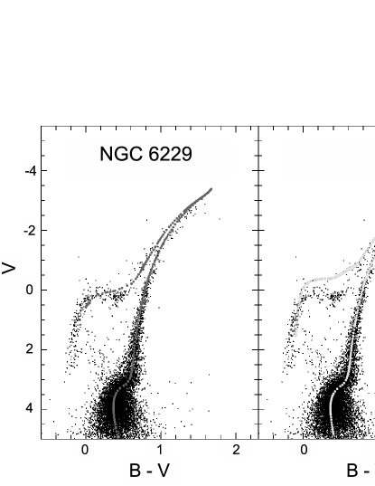
5mm normal

Figure 2: Comparison of the $C$–$M$ diagram $V$–$(B-V)$ for NGC 6229 piotto:Khamidullina_n with the isochrones from Bertelli et al. bert1:Khamidullina_n . The left panel shows the isochrone $\log\leavevmode\nobreak\ t=10.1$, $Y=0.26$, $Z=0.0004$ used in the GC spectrum modelling. On the right, the isochrone $\log\leavevmode\nobreak\ t=10.1$, $Y=0.3$, $Z=0.0004$ (see Section 3.1) is shown for comparison.

5mm

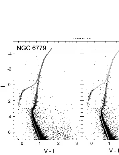
Figure 3: Comparison of the $C$–$M$ diagram $I$–$(V-I)$ for NGC 6779 sarajedini:Khamidullina_n with the isochrones from bert1:Khamidullina_n . The left panel shows the isochrone $\log\leavevmode\nobreak\ t=10.1$, $Y=0.23$, $Z=0.0001$ used in the GC spectrum modelling. On the right, the isochrone $\log\leavevmode\nobreak\ t=10.15$, $Y=0.23$, $Z=0.0001$ is shown for comparison.

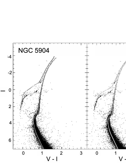
5mm normal

Figure 4: Comparison of the $C$–$M$ diagram $I$–$(V-I)$ for NGC 5904 piotto:Khamidullina_n with the isochrones from bert1:Khamidullina_n . The left panel shows the isochrone $\log\leavevmode\nobreak\ t=10.1$, $Y=0.30$, $Z=0.001$ used in the GC spectrum modelling. On the right, the isochrone $\log\leavevmode\nobreak\ t=10.15$, $Y=0.26$, $Z=0.001$ (see Section 3.1) is shown for comparison.

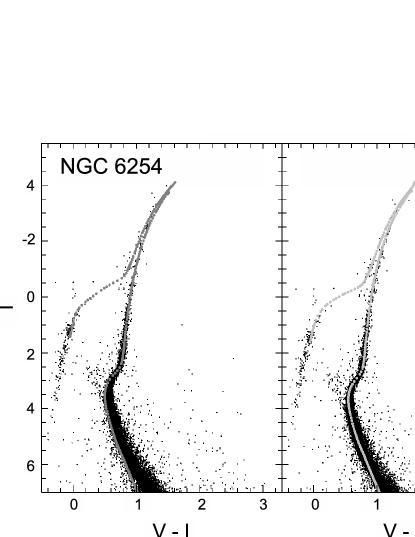
5mm normal

Figure 5: Comparison of the $C$–$M$ diagram $I$–$(V-I)$ for NGC 6254 sarajedini:Khamidullina_n with the isochrones from bert1:Khamidullina_n . The left panel shows the isochrone $\log\leavevmode\nobreak\ t=10.05$, $Y=0.30$, $Z=0.0004$, used in the GC spectrum modelling. On the right, the isochrone $\log\leavevmode\nobreak\ t=10.15$, $Y=0.26$, $Z=0.0004$ is shown for comparison.

The derived results of isochrone selection using the $C$–$M$ diagram and the spectra for the globular clusters under study are shown in the left panels of Figs. 3–5. On the right-hand side, isochrone positions with varied parameters are presented. For NGC 6229 the variation of the isochrone position with increasing $Y$ is shown, for NGC 6779—with increasing age, and for NGC 5904 and NGC 6254—with the variation of $Y$ and age. For the last two clusters, isochrones with parameters close to those estimated in VDBerg90g:Khamidullina_n are presented. Distance and $E(B-V)$ were changed according to variations of the above mentioned parameters. All GCs have certain stars and sequences which cannot be described by isochrones. They are hot blue HB stars, blue stragglers, certain bright stars deviating from the red giant branch (background objects or asymptotic giant branch stars). In Section 3.3.2 we discuss the significance of the listed deviations during the analysis of the correspondence of theoretical spectra calculated with the specified isochrones to the observed ones. Figs. 6–9 show the spectral regions with hydrogen lines calculated with the parameters of isochrones which are used in Figs. 3–5. As the final values of [Fe/H], $t$ and $Y$, we adopted those that best describe the observed spectra.

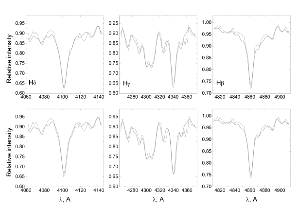
5mm normal

Figure 6: The fit of the isochrone parameters to the observed spectrum of NGC 6229 (the profiles of the H$\beta$, H$\gamma$, H$\delta$ lines). The three upper panels show the applied model $\log\leavevmode\nobreak\ t=10.1$, $Y=0.26$, $Z=0.0004$ (see the corresponding $C$–$M$ diagram on the left of Fig. 3). The three lower panels show the model $\log\leavevmode\nobreak\ t=10.1$, $Y=0.30$, $Z=0.0004$ (the right-hand side of Fig. 3) for comparison.

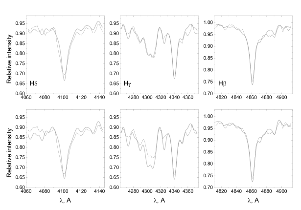
5mm normal

Figure 7: The fit of the isochrone parameters to the observed spectrum of NGC 6779 (the profiles of the H$\beta$, H$\gamma$, H$\delta$ lines). The three upper panels show the applied model $\log\leavevmode\nobreak\ t=10.1$, $Y=0.23$, $Z=0.0001$ (see the corresponding $C$–$M$ diagram on the left of Fig. 3). The three lower panels show the model $\log\leavevmode\nobreak\ t=10.15$, $Y=0.23$, $Z=0.0001$ (the right-hand side of Fig. 3) for comparison.

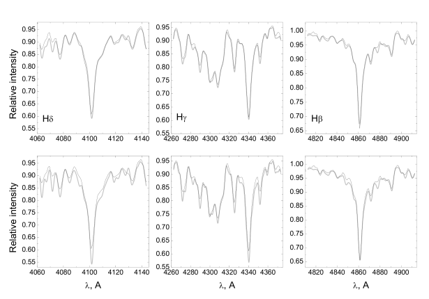
5mm normal

Figure 8: The fit of the isochrone parameters to the observed spectrum of NGC 5904 (the profiles of the H$\beta$, H$\gamma$, H$\delta$ lines). The three upper panels show the applied model $\log\leavevmode\nobreak\ t=10.1$, $Y=0.30$, $Z=0.001$ (see the corresponding $C$–$M$ diagram on the left of Fig. 5). The three lower panels show the model $\log\leavevmode\nobreak\ t=10.15$, $Y=0.26$, $Z=0.001$ (the right-hand side of Fig. 5) for comparison.

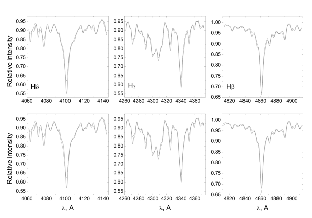
5mm normal

Figure 9: The fit of the isochrone parameters to the observed spectrum of NGC 6254 (the profiles of the H$\beta$, H$\gamma$, H$\delta$ lines). The three upper panels show the applied model $\log\leavevmode\nobreak\ t=10.05$, $Y=0.30$, $Z=0.0004$ (see the corresponding $C$–$M$ diagram on the left of Fig. 5). The three lower panels show the model $\log\leavevmode\nobreak\ t=10.15$, $Y=0.26$, $Z=0.0004$ (the right-hand side of Fig. 5) for comparison.

The results of isochrone selection for the thoroughly studied clusters NGC 5904 and NGC 6254 (Figs. 5 and 5) agree with the quantities from the literature (Table 3) harris96:Khamidullina_n ; vandenberg:Khamidullina_n . The differences in age estimates do not exceed 1 Gyr. However, the [Fe/H] value is regularly underestimated by $0.1$–$0.3$ dex for all the clusters except NGC 6779. For the two tested clusters, the helium abundance was found to be higher than in the photometric results of VandenBerg et al. vandenberg:Khamidullina_n . The $\alpha$-element abundance for NGC 6254 that we measured turned out to be $0.2$–$0.3$ dex lower than the value reported in the literature. On the whole, our errors of the determination of the main cluster parameters do not exceed 20%.

Table 3: Comparison of the values taken from the literature harris96:Khamidullina_n ; vandenberg:Khamidullina_n and those determined by us using photometric and spectroscopic methods: [Fe/H] (in dex), helium abundance $Y$, age $t$ (in Gyr), $\alpha$-element abundance $[\alpha/Fe]=\left([Mg/Fe]+[Ca/Fe]\right)/2$ (in dex), and average microturbulence velocity for each cluster $\xi_{\rm turb}$ in km s^-1. The parameter ${\rm HBR}=(B-R)/(B+V+R)$ harris96:Khamidullina_n characterizes the number of stars in the blue and red regions of the horizontal branch and in the Hertzsprung gap

Parameter	NGC 6229	NGC 6779	NGC 5904	NGC 6254	Ref.
[Fe/H], dex	$-1.43$	$-1.94$	$-1.27$	$-1.52$	[1]
${\rm HBR}$	$0.24$	$0.98$	$0.31$	$0.98$	[1]
$[\alpha/Fe]$	–	–	$0.21$	$0.26$	[37]
$[\alpha/Fe]$	–	–	$0.31$	$0.39$	[31]
$[Fe/H]$	–	$-2.00$	$-1.33$	$-1.57$	[17]
$t$	–	$12.75\pm 0.50$	$11.50\pm 0.25$	$11.75\pm 0.38$	[17]
$Y$	–	$0.25$	$0.25$	$0.25$	[17]
$[Fe/H]_{\rm isochr.}$	$-1.74$	$-2.35$	$-1.33$	$-1.74$	ours
$t_{\rm isochr.+spectra}$	$12.6$	$12.6$	$12.6$	$11.2$	ours
$Y_{\rm isochr.+spectra}$	$0.26$	$0.23$	$0.30$	$0.30$	ours
$[Fe/H]_{\rm spectra}$	$-1.65$	$-1.9$	$-1.6$	$-1.75$	ours
$[\alpha/Fe]_{\rm spectra}$	$0.28$	$0.08$	$0.35$	$0.025$	ours
$\xi_{\rm turb}$	$2.1$	$2.1$	$2.1$	$1.8$	ours

0mm normal NGC 6229 NGC 5904 NGC 5904roediger:Khamidullina_n Elem. [X/Fe] $\sigma$ [X/Fe] $\sigma$ [X/Fe] $\sigma$ C $-0.05$ $0.15$ $-0.20$ $0.10$ $-0.48$ $0.26$ N $0.35$ $0.25$ $0.20$ $0.20$ $0.68$ $0.59$ O $0.35$ $0.30$ $0.20$ $0.30$ $0.15$ $0.27$ Na $0.25$ $0.20$ $0.20$ $0.15$ $0.19$ $0.26$ Mg $0.15$ $0.15$ $0.40$ $0.15$ $0.33$ $0.10$ Ca $0.40$ $0.15$ $0.20$ $0.10$ $0.28$ $0.11$ Ti $0.40$ $0.25$ $0.20$ $0.20$ $0.22$ $0.10$ Cr $0.15$ $0.20$ $0.10$ $0.15$ $-0.08$ $0.19$

Table 4: Derived abundances [X/Fe] (in dex) and their dispersion $\sigma$ (in dex) for NGC 6229 and NGC 5904. The corresponding values from roediger:Khamidullina_n are listed in the last column.

0mm normal NGC 6779 NGC 6254 NGC 6254pritzl05:Khamidullina_n Elem. [X/Fe] $\sigma$ [X/Fe] $\sigma$ [X/Fe] $\sigma$ C $-0.15$ $0.15$ $-0.15$ $0.10$ $-0.77$ $0.37$ N $-0.10$ $0.25$ $0.25$ $0.20$ $1.01$ $0.45$ O $-0.20$ $0.30$ $0.40$ $0.30$ $0.23$ $0.24$ Na $-0.20$ $0.20$ $0.25$ $0.15$ $0.17$ $0.27$ Mg $-0.10$ $0.15$ $0.05$ $0.15$ $0.44$ $0.13$ Ca $0.25$ $0.15$ $0.00$ $0.10$ $0.33$ $0.11$ Ti $0.10$ $0.25$ $0.45$ $0.20$ $0.26$ $0.12$ Cr $-0.10$ $0.20$ $-0.09$ $0.15$ $0.001$ $0.15$

Table 5: Derived abundances [X/Fe] (in dex) and their dispersion $\sigma$ (in dex) for NGC 6779 and NGC 6254. The corresponding values from pritzl05:Khamidullina_n are listed in the last column.

However, we note the common problem (in the literature and ours) of describing the cluster $C$–$M$ diagram using the evolutionary tracks and isochrones. Actually, none of the presented isochrones describes the $C$–$M$ diagram of the cluster in all details. We selected the isochrones that provide the best agreement between the observed and theoretical spectra calculated using the distribution of stars by mass, $\log\leavevmode\nobreak\ g$, and $T_{\rm eff}$ corresponding to these isochrones. Note that besides the above-mentioned particular stars with noticeable deviations from the isochrone, in some other cases (see, e.g., Fig. 5), the spectrum analysis implies a small shift of the MS turnoff point toward higher temperatures or a change of the HB position. For NGC 5904 such changes may be caused by the increased percentage of hot blue HB stars, the EHB (Extended Horizontal Branch), and/or blue stragglers caught in the spectrograph slit.

3.2 Modelling of Stellar Spectra

The number of stars with a given mass is calculated according to the Chabrier mass function chabrier:Khamidullina_n . For obtaining the synthetic spectra of plane-parallel, hydrostatic stellar atmospheres for the derived isochronic parameters ($T_{\rm eff}$, $\log g$, [Fe/H]), we use the CLUSTER sharina:Khamidullina_n software. Model atmospheres are computed by interpolating the grids of Castelli and Kurucz cast1:Khamidullina_n according to the technique described in sule2:Khamidullina_n . For normalization we model two spectra simultaneously: (1) with the allowance for atomic lines and molecular bands in the spectral range covered, and (2) without it. Thus, the synthetic spectra are derived by dividing (1) by (2). Note that during the modelling of all spectra, a constant wavelength step of $\Delta\lambda=0.05$ Åwas assumed, which ensures errors of the flux in the continuum and in the lines no greater than $0.005\%$ of the residual intensity. During the analysis of moderate-resolution spectra (${\rm FWHM}\leq 5$ Å), it is possible to investigate not only the individual lines but also broad blends $\Delta\lambda\geq 5$ Å consisting of lines and bands of many atoms and molecules. Therefore, to determine the parameters and abundances of GCs, it is necessary to achieve the best fit between theoretical and observed spectra in the whole studied range. As the analysis in sharina:Khamidullina_n with $S/N>100$ showed, this approach allows us to determine the cluster parameters and the abundances of about 10 chemical elements. Our abundances, determined by the strong Ca, Mg, Fe, CH lines and blends, the majority of the Na, Al, Ba, Sr lines, and all the lines with $\lambda>5300$ Å, are differential, as the empirical oscillator strengths $gf$, derived in shim11:Khamidullina_n by the solar spectrum analysis, are used. For the rest of the lines, theoretical values of $gf$ are used which can cause, according to the analysis of Shimanskaya et al. shim11:Khamidullina_n , a systematic abundance underestimation of up to 0.07 dex. A common microturbulence velocity $\xi_{\rm turb}$ for all the GC stars (Table 3) is derived from the best fit between the strong and weak iron lines in the theoretical and observed spectra. Figures 10–13 show examples of Fe line variations at different $\xi_{\rm turb}$ values. Table 3 shows the $\xi_{\rm turb}$ values derived by us. Note that the use of a common value of $\xi_{\rm turb}$ for all the cluster stars is not quite proper. However, the analysis of the integrated spectra of GCs does not allow us to derive a dependence of $\xi_{\rm turb}$ on stellar parameters. Moreover, the main contribution to the optical spectra is made by the stars located at the MS turnoff point at $T_{\rm eff}=6200$–$7500$ K and by the brightest asymptotic branch giants. For such stars, the microturbulence velocity is within the range of $\xi_{\rm turb}=1.8$–$2.4$ km s^-1. That is why the use of a common value of $\xi_{\rm turb}$ cannot cause any significant errors in the abundance of chemical elements. The macroturbulence and rotation of individual cluster stars are neglected in our calculations, as those effects amount to less than $30$ km s^-1 and, consequently, are insignificant at our resolution. For the same reason, we do not consider the velocity dispersion of the stars within the cluster.

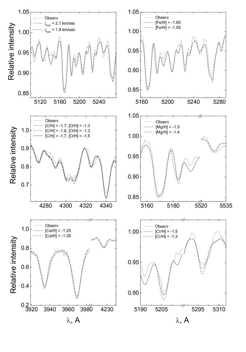
5mm normal

Figure 10: Determination of microturbulence velocity $\xi_{\rm turb}$ and Fe, C, Mg, Ca, and Cr abundances for NGC 6229. The observed spectrum (solid lines) and theoretical spectra (dashed, dashed-and-dotted, and dotted lines) calculated for different [X/H] values with constant abundances of other elements (see Sections 3.2, 4) are shown.

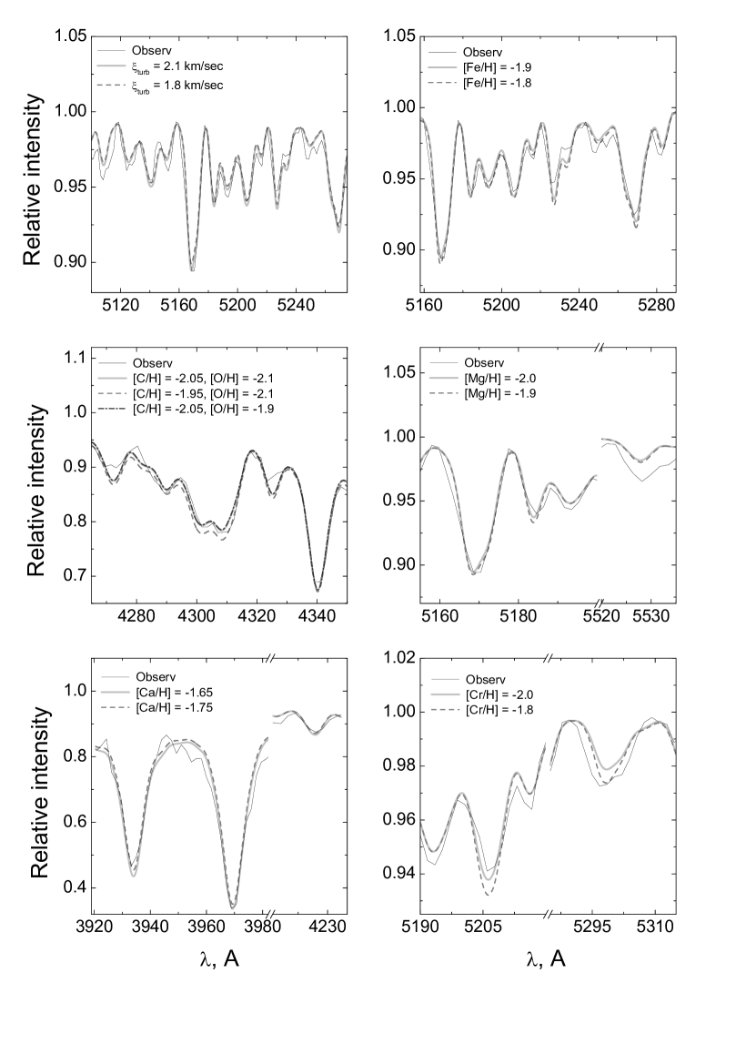
5mm normal

Figure 11: The same as in Fig. 10, but for NGC 6779.

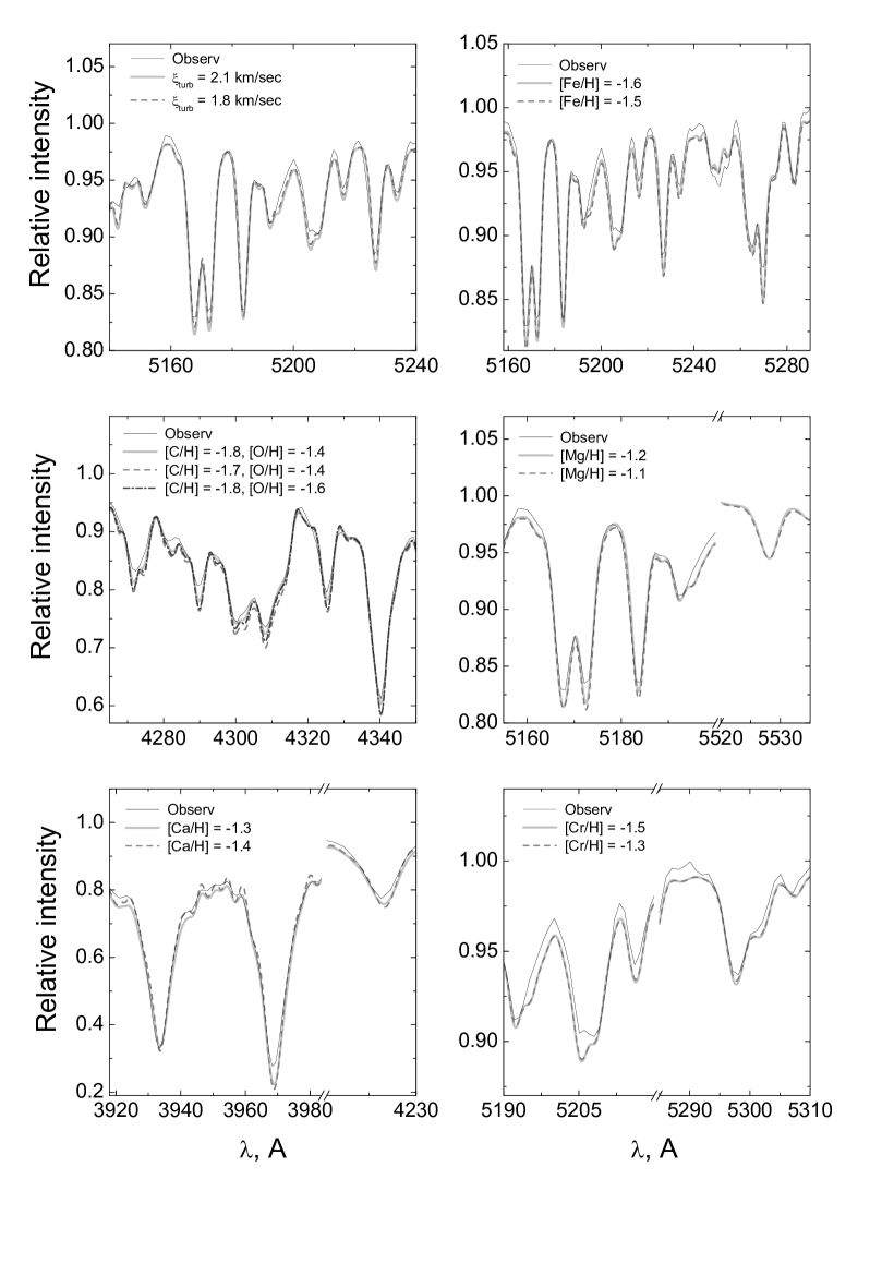
5mm normal

Figure 12: The same as in Fig. 10, but for NGC 5904.

5mm normal

Figure 13: The same as in Fig. 10, but for NGC 6254.

Fitting the continuum of the observed spectra to the theoretical ones is conducted by the successive use of the following digital filters (see the description of MIDAS for details): (1) determining the maximum spectral intensity within a specified wavelength range ($5\,{\rm FWHM}$), (2) smoothing filter (running median) with a radius of $6\,{\rm FWHM}$, where $\rm FWHM$ denotes the spectral resolution of the spectrograph in Å.

The contribution of the stars of different types to the integrated GC flux is described by the example of NGC 6229 in Fig. 14. This cluster has an HB of an intermediate type, although its blue and red ends are densely populated with stars. Hot blue HB stars determine the width and intensity of the hydrogen lines. These objects contribute up to 40$\%$ of the energy distribution in the blue region of the investigated spectral range. Red giants, dominating in its red region, are the main source of molecular bands and lines of neutral atoms of heavy elements. Note that the molecular lines in the sum spectrum of the stars in the red giant branch are much more noticeable than in the spectrum of the MS and subgiants branch stars. As a result, the integrated spectrum of the whole cluster noticeably differs from the spectra of all its components.

5mm normal

Figure 14: The contribution of different types of stars to the integrated GC radiation. The example of NGC 6229 is considered.

3.3 Abundance Determination

Variations of [Fe/H], $\log\leavevmode\nobreak\ g$, and $T_{\rm eff}$ allow us to calculate the spectra of various cluster stars. Summing up these spectra taking into account the stellar mass functions produces the total synthetic spectrum of a GC.

The average chemical abundances in the atmospheres of GC stars are determined by matching the observed and theoretical line profiles, line blends, and molecular bands. As explained in the previous paragraph, the resolution of our spectra does not allow us to determine chemical abundances from individual lines. In view of that, we adopted such abundances for each element for which all the blends (including the lines of this element in the studied wavelength interval) are best described by the theoretical spectrum.

First, we determine the chemical abundance of the elements whose lines and/or molecular bands dominate in the spectra which allows us to obtain [X/H] values with an accuracy of $\Delta[X/H]\sim 0.1$–$0.2$ dex. These elements are Fe, Ca, Mg, C. The line profiles of Ti, Cr, Co, Mn, N are analyzed by varying their abundances using previously derived fixed abundances of the elements from the first group. The accuracy of chemical abundance estimation for the elements of the second group, the lines of which are much weaker and more blended than the lines of the elements from the first group, is about $0.2$–$0.3$ dex. When we use moderate-resolution spectra, the individual elements do not have any noticeable details in the observed wavelength range, but they influence the molecular and ionization equilibrium of other elements. Oxygen belongs to such elements; as its abundance increases, a part of atomic carbon participates in the formation of the CO molecule which reduces the intensity of the CN and CH molecular bands. The elements Al, Si, V, Ni influence the electronic equilibrium in stellar atmospheres only slightly, and also do not have observable lines at moderate resolution. Na should also be included in this group, as its resonance lines are heavily distorted by interstellar lines and are unsuitable for analysis.

4 RESULTS

This is the first time that the chemical abundances for the clusters NGC 6229 and NGC 6779 have been derived. Tables 3–5 and Figs. 10–13 show the final results for them and for the comparison clusters NGC 5904 and NGC 6254. Table 3 summarizes the GC fundamental parameters: age, helium abundance, iron [Fe/H] and $\alpha$-element abundance averaged over the GC. Tables 4 and 5 show the abundances of individual chemical elements. Figs. 6–9 show the results of the comparison of the observed and theoretical H$\beta$, H$\gamma$, H$\delta$ line profiles, calculated based on the isochrones with the parameters derived from the photometric data (see above). Figs. 10–13 show the profiles of the lines and molecular bands of different chemical elements that were used to estimate their abundances. For each element, two–three variants of the line profiles with different abundances are presented for reliability assessment and accuracy check. It is necessary to note that when fitting the theoretical spectrum to the observed one, we assume that the light from GC stars in the main evolutionary stages is adequately represented in these two spectra. It is also assumed that the observed spectrum is not distorted by background objects. In reality, the last condition is not always met, especially in the case of GCs close to the Galactic plane. Observations with different slit orientations allow us to eliminate the distortions caused by background stars in most cases. The spectra of test GCs from Schiavon et al. schiavon:Khamidullina_n were derived using the long-slit scanning method, and, thus, they may contain such distortions.

As was mentioned in the Introduction, age, [Fe/H], and $Y$ were estimated using deep photometry results from the literature. Table 3 shows the summary of those estimates. Generally, our results of the above-mentioned estimation of these parameters, derived by means of cluster spectrum analysis, agree with the ones from the literature. However, there are a number of discrepancies. Our age estimate for the well studied GC NGC 5904 exceeds the value derived in vandenberg:Khamidullina_n by 0.9 Gyr, and the helium abundance is excessive. These parameters are determined by the H I line profile analysis, as explained in Section 3.2. Our [Fe/H] values, derived using the spectroscopic method, are in most cases smaller by 0.2–0.3 dex than those from the literature, derived by the $C$–$M$ diagram analysis. It is unlikely that these discrepancies are caused by background stars caught in the slit. The projected vicinities of the investigated clusters mainly contain stars of the Galactic disk with close-to-solar metallicities. We have not detected any emissions in the observed cluster spectra. Thus, the noted differences are likely associated with the distinctions of the applied methods and models. When analyzing the photometric data, the errors of color indices and distances to the clusters, and also the use of theoretical isochrones from different authors produce random and systematic shifts in the derived parameters gallart:Khamidullina_n . The use of different atomic and molecular data sets, different model atmospheres for the stars, and different principles of modelling simple stellar populations leads to differences in the abundance estimates and cluster evolutionary parameters.

Tables 4 and 5, and Figs. 15 and 16 show the comparison of our abundance estimation results for different elements and the results from pritzl05:Khamidullina_n and roediger:Khamidullina_n for the well studied clusters NGC 5904 and NGC 6254. The abundance differences are greater than the given errors only for C and N. A possible explanation is that we analyze the average chemical abundance of the whole cluster and not only of the high-luminosity stars, as the majority of the authors do. The products of the CNO cycle could be brought up to the surface of these stars, and this may cause an increase in the nitrogen abundance and a decrease of that of carbon. Note that the considerable contribution of red giants to the cluster spectrum probably increases the distortions of the estimated C and N abundances, but their amplitude should be much smaller than in the investigation of individual stars. There are also significant differences in the Mg and Ca abundances for NGC 6254. Considerable variations of C, N, O, Mg, Na, and Al from star to star were found for a number of massive Galactic GCs gratton04:Khamidullina_n . In one and the same cluster, one can often observe two or more stellar populations with different chemical abundances forming different sequences in the $C$–$M$ diagram. This is explained by the mixing of matter after the CNO cycle. The Mg abundance variations after such processes are expected to be around $\Delta Mg\leq 0.3$ dex pritzl05:Khamidullina_n . Note once again that the estimates from the literature are based mainly on the investigations of red giants, which are not the true indicators of GC initial abundances because of the mixing of matter, to which their atmospheres are liable (the first dredge-up). Therefore, more detailed theoretical and observational investigations are necessary in order to check how much the cluster abundance variations depend on the physical characteristics of the studied stars.

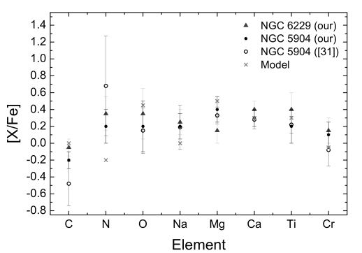
5mm normal

Figure 15: A comparison of the chemical abundances in NGC 6229 and NGC 5904 according to the results of this paper. The open circles denote the data from roediger:Khamidullina_n .

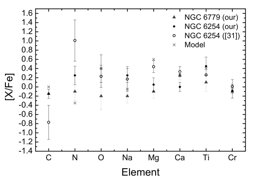
5mm normal

Figure 16: A comparison of the chemical abundances in NGC 6779 and NGC 6254 according to the results of this paper. The open circles denote the data from roediger:Khamidullina_n .

Almost all our estimated abundances agree with the theoretical calculations of the models of the chemical evolution of the Galaxy and also with the average values for dwarfs at the given metallicity (see samland:Khamidullina_n ; alibes:Khamidullina_n ; kobayashi:Khamidullina_n ). However, the scatter of the observed values, with which model characteristics are compared, is often large.

Carbon is produced in the triple $\alpha$-process with hydrostatic He burning in stars of various masses. The average abundance of C in halo and disk dwarfs varies little with time (does not depend on [Fe/H]): $[C/Fe]\sim 0$ alibes:Khamidullina_n . We have derived similar values.

The nitrogen abundance decreases with metallicity as massive stars do not produce primary N. With the [Fe/H] increase, the production of the so-called secondary N by moderate-mass stars increases until the Fe production by Ia supernovae compensates this process at $[Fe/H]\sim-1$. The theoretical [N/Fe] values vary from $0$ to $-0.5$ in the following range: $-2<[Fe/H]<1$. Our estimates are closer to the theoretical ones than the data from the literature for the giants in NGC 5904 and NGC 6254.

Oxygen, as the majority of other $\alpha$-elements, is produced by massive stars only. $[O/Fe]\sim 0.5$ at $[Fe/H]\leq 1$. Our values correspond quite well to those calculations, except for NGC 6779, for which we obtained lower abundance estimates for the other $\alpha$-elements as well. There were no emissions or noticeable distortions from background stars detected in the spectra. However, one cannot exclude the latter possibility for NGC 6779, which is closer to the plane of the Milky Way than the other three clusters.

The evolution of the abundance of magnesium as a function of metallicity is impossible to explain only by its formation in massive stars (alibes:Khamidullina_n and references therein). The theoretical [Mg/Fe] values in the range of $-2<[Fe/H]<1$ are usually a little lower than the observed ones. Our results agree better with the theoretical values. However, the scatter of the observed data is large. On the whole, one can conclude that the [Mg/Fe] values for the selected clusters except NGC 6779 are within the normal range.

The value of [Ca/Fe] is in close agreement with theory for all the selected clusters except NGC 6254. We estimated the abundance of this element not only from the Ca I $\lambda\leavevmode\nobreak\ 4226$ Å resonance line but also from the H and K Ca II lines, the profiles of which vary greatly depending on the selected isochrone, as these profiles are determined not only by the Ca content but also by age, $Y$, and [Fe/H]. Thus, an error in the [Ca/Fe] estimate is possible, but much less probable than the possible errors for the elements heavier than Ca, which have no broad spectral features.

Tables 4 and 5 and Figs. 15 and 16 show that, on the whole, the chemical abundances for NGC 5904 and NGC 6254 are similar to the ones for NGC 6229 and NGC 6779. The published values of [Fe/H] for NGC 6779 and NGC 6254 are smaller than the same values for NGC 6229 and NGC 5904. This fact, in view of the similarity of the horizontal branches of NGC 6229 and NGC 5904, and also of NGC 6779 and NGC 6254, has been a reason for associating the clusters of higher metallicity with the young Galactic halo, and clusters of lower metallicity—with the old one mars:Khamidullina_n . Following our results (see Table 3), there are no two objects out of the four investigated that are totally similar in all parameters. The similarity in the chemical abundances is indicative of the fact that they belong to the old Galactic halo, in which nucleosynthesis proceeded according to the main evolutionary stages under the influence of SN II and SN Ia supernovae. In order to associate the clusters with one or another Galactic subsystem, a more detailed analysis of the chemical, kinematic, and structural characteristics is necessary.

5 CONCLUSIONS AND SUMMARY

The method we used for modelling and analysis of the integrated spectra of the clusters was previously discussed in sharina:Khamidullina_n . In this paper we expanded it by including the investigation of the cluster $C$–$M$ diagrams and their detailed comparison with the theoretical isochrones. Now, as a result, this method combines the possibilities of using both the spectroscopic, integrated along the slit data, and photometric data on the stellar populations of the clusters. We use the results of deep stellar photometry from the literature to select an isochrone that best fits the cluster $C$–$M$ diagram. The summing-up of the stellar synthetic blanketed spectra, calculated using model atmospheres, is conducted using the stellar luminosity function of Chabrier chabrier:Khamidullina_n . The matching of the theoretical and observed cluster spectra is carried out iteratively. Initially, the distribution of cluster stars by mass, radius, and $\log\leavevmode\nobreak\ g$ is preset using the literature data on the theoretical isochrone which fits best the observed $C$–$M$ diagram. For the specification of stellar ages and helium abundances, the profiles of the hydrogen lines are analyzed, because they practically do not depend on other parameters. The abundance of iron is then varied, the lines of which prevail in the optical spectrum even at a low metallicity. Upon achieving the closest agreement in these three parameters, the abundances of the $\alpha$-elements Mg, Ca, and C are derived. The molecular bands and lines of these elements are the most significant in the spectrum. For the determination of the abundances of other elements, complex blends consisting of many lines are used. As a result, the abundances of about 10 elements are estimated. Note that the use of a considerable number of lines with empirical $gf$ values allows us to obtain differential abundances (i.e., bound to the $gf$ values of solar spectral lines) of Ca, Mg, Fe, C, and, in some cases, other elements.

In this paper, we determined the ages, specific helium abundances $Y$, and abundances of Fe, C, N, O, Na, Mg, Ca, Ti, and Cr for the following four Galactic GCs using the developed method: NGC 6229, NGC 6779, NGC 5904, NGC 6254. The chemical abundances for the first two objects were estimated with a spectroscopic method for the first time. According to our estimates, these GCs turned out to be about 1 Gyr younger than NGC 5904 and NGC 6254, which are accepted in the literature as their analogues. The helium abundance that we determined for the last two clusters is higher ($Y=0.30$) than the one in the literature. The clusters NGC 6229 and NGC 6779 show the values $Y=0.23$ and $Y=0.26$ respectively, which are closer to the value of the primordial helium abundance in the Universe $Y=0.25$ komatsu11:Khamidullina_n . The $\alpha$-element abundancesin the metal-poor ($[Fe/H]\sim-1.6$) NGC 6229and NGC 5904 turned out to be high($[\alpha/Fe]=0.28$–$0.35$) as in the old massive globular clusters of the Galaxy; massive type II supernovae contributed greatly to their chemical enrichment. However, the $\alpha$-element abundances in the investigated clusters with low central density, NGC 6779 and NGC 6254, turned out to be quite low ($[\alpha/Fe]=0.08,0.025$), while their metallicity was low ([$Fe/H]=-1.9,-1.7$). Such $[\alpha/Fe]$ values are not typical for low metallicity Galactic clusters. For this reason, the search for a dependence of the chemical abundance of GCs on their structure and kinematic characteristics can be the subject of future investigations. A comparison of the derived abundances and the literature values for the well studied GCs NGC 5904 and NGC 6254 showed that our measurements are consistent with the corresponding average estimates from the literature for cluster giants with the average accuracy of about $0.15$ dex, except for C and N. This is probably due to the difference between the average chemical composition in the stellar atmospheres for the whole cluster, derived in this paper, and the chemical composition of the atmospheres of high-luminosity stars listed in the literature. The products of the CNO cycle can be transported to the surface of such stars, and their study does not provide accurate information on the primary chemical abundance of GCs.

The values of [Fe/H], $Y$, and age which we derived by spectroscopic analysis allow us to evaluate the true correlation between the observed $C$–$M$ diagram and the corresponding theoretical isochrone. At present, there is no possibility of combining the deep stellar photometry data with the spectroscopic methods of estimating the element abundances and evolutionary parameters when analyzing the characteristics of stellar populations in extragalactic GCs. Thus, our investigation provides essential data for understanding the characteristics of GCs in remote galaxies.

Translated by N. Oborina