Phonon statistics in an acoustical resonator coupled to a pumped two-level emitter

Abstract

The concept of an acoustical analog of the optical laser has been developed recently both in theoretical as well as experimental works. We discuss here a model of a coherent phonon generator with a direct signature of quantum properties of the sound vibrations. The considered setup is made of a laser driven quantum dot (QD) embedded in an acoustical nanocavity. The system’s dynamics is solved for a single phonon mode in the steady-state and in the strong QD-phonon coupling regime beyond the secular approximation. We demonstrate that the phonon statistics exhibits quantum features, i.e. sub-Poissonian phonon statistics.

I Introduction

Sub-Poissonian statistics of vibrational states is a pure quantum propriety of an oscillating system. The domain of this statistics starts at the limit of a classical coherent state having a Poissonian distributed quanta and may end up with a pure Fock state at the other limit. Studies on the quanta statistics had already revealed many pure quantum features for different physical systems and remarkable results were achieved in a large spectrum of photonic quantum electrodynamics’s (QED) applications remp as well as in Bose-Einstein condensate’s (BEC) physics chuu ; jacq . More recently, successful experiments in cooling and detection of mechanical systems in the near ground state domain roch ; conn ; chan enhanced a particular interest in the research of similar features in the acoustical domain, due to bosonic quantification of the sound’s vibrations.

Earlier experiments in laser generation of coherent phonons in different bulk materials kutt ; bart ; ezza were succeeded by new optomechanical and electromechanical setups in phonon QED, achieving important experimental results in the acoustical analog of the optical laser by using piezoelectrically excited electromechanical resonators mahb and laser driven compound microcavities grud or trapped ions vaha . In the meantime, theoretical models propose improvements in the background theory of the experiments like the PT-symmetry approach jing and two cavity optomechanics wang , as well as new possible setups using vibrating membranes wang ; wu , quantum dots embedded in semiconductor lattices kab1 ; kab2 ; okuy and BECs under the action of magnetic cantilever bhat . Moreover, quantum features like sub-Poissonian distributed phonon fields have been already predicted in optomechanical setups based on vibrating mirrors roqu ; nati and in single-electron transistors merl as well as phonon antibunching okuy , squeezing roqu ; kron and negative Wigner function of phonon states qian . In addition to increasing performances of the optomechanical devices aspe , reports on the art-of-the-state of acoustical cavities trig ; lanz ; soyk have shown good phonon trapping in bulk materials with high cavity quality factors, thus leading to the concept of acoustical analog of photon cavity-QEDs (cQED).

In this article, we study the model of a coherent phonon generator in a setup consisting of a qubit embedded in an acoustical cavity involving strong QD-phonon-cavity coupling regime. The qubit, i.e. a two-level quantum dot, is driven by an intense laser field and acts as a phonon source. Under action of laser light the electron jumps from the QD’s valence band to the conductance band leaving a “hole” in the valence band. The created exciton (electron-hole) represents the QD’s excited state and interacts with the acoustical vibrations, thus, creating or annihilating phonons in the cavity. We demonstrate that in analogy with recent experiments in photon cQED kim the strong qubit-resonator couplings may reveal additional quantum phenomena in the phonon cQED’s domain. Particularly, we show that in this regime the generated steady-state phonon field obeys sub-Poissonian phonon statistics.

This paper is organized as follows. In Sec. II a detailed description of the model is given, i.e., after an introduction of the used nomenclature we focus on simplifying the system’s Hamiltonian in order to arrive at an easy solvable master equation for the reduced density operator of the QD-phonon system. In Sec. III, we present a general overview over the model’s results and we further discuss the important aspects of the study. The Summary is given in Sec. IV.

II Theoretical framework

A two-level laser-pumped semiconductor quantum dot is embedded in an acoustical nanocavity (see also kab1 ; kab2 ). The QD’s transition frequency between its ground state $|g\rangle$ and the excited state $|e\rangle$ is denoted by $\omega_{qd}$. The excited QD may spontaneously emit a photon with $\gamma$ being the corresponding decay rate, see Fig. 1. For a more realistic case, we introduce the dephasing losses rate through $\gamma_{c}$. The single mode cavity phonons of frequency $\omega_{ph}$ are described by the anihilation $(b)$ and the creation $(b^{\dagger})$ operators, respectively. The system’s Hamiltonian is:

$$H = \hbar\omega_{qd}S_{z}+\hbar\omega_{ph}b^{\dagger}b+\hbar\Omega(S^{+}e^{-i\omega_{L}t}+S^{-}e^{i\omega_{L}t})$$ (1)

$$+ \hbar gS^{+}S^{-}(b^{\dagger}+b),$$

where the QD’s operators are defined as: $S^{+}=|e\rangle\langle g|$, $S^{-}=|g\rangle\langle e|$ and $S_{z}=\frac{1}{2}\left(|e\rangle\langle e|-|g\rangle\langle g|\right)$ obeying the standard commutation relations for SU(2) algebra. The first two terms correspond, respectively, to the unperturbed QD and to the free single mode phonon Hamiltonians. The third term corresponds to the QD-laser interaction within rotating wave and dipole approximations whereas $\omega_{L}$ is the laser frequency. The last term describes the QD-phonon-cavity interaction with $g$ being the coupling strength constant.

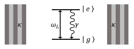
Figure 1: (color online) The schematic of the investigated model: A two-level QD is fixed in a multilayered structure forming the acoustical nanocavity. The QD is pumped near resonance with a coherent laser source of frequency $\omega_{L}$. The emitter may spontaneously emit a photon at a decay rate $\gamma$ while the cavity phonon damping rate is denoted by $\kappa$ (see also Ref. soyk ).

In what follows, we describe the Hamiltonian in a frame rotating at the laser frequency $\omega_{L}$ and apply the dressed-state transformation:

$$|+\rangle = \sin{\theta}|g\rangle+\cos{\theta}|e\rangle,$$

$$|-\rangle = \cos{\theta}|g\rangle-\sin{\theta}|e\rangle,$$ (2)

where $2\theta=\arctan{(2\Omega/\Delta)}$ while $\Delta=\omega_{qd}-\omega_{L}$ is the detuning of the laser from the QD’s transition frequency. The dressed-state system’s Hamiltonian becomes then:

$$H = \hbar\bar{\Omega}R_{z}+\hbar\omega_{ph}b^{\dagger}b+\hbar g(b^{\dagger}+b)\{\sin^{2}{\theta}\,R_{--}$$ (3)

$$+ \cos^{2}{\theta}\,R_{++}-\frac{\sin{(2\theta)}}{2}(R^{+}+R^{-})\},$$

where $\bar{\Omega}=\sqrt{\Omega^{2}+({\Delta/2})^{2}}$. The new QD’s operators are: $R^{+}=|+\rangle\langle-|$, $R^{-}=|-\rangle\langle+|$, $R_{++}=|+\rangle\langle+|$, $R_{--}=|-\rangle\langle-|$ and $R_{z}=R_{++}-R_{--}$ satisfying the commutation relations $[R^{\pm},R^{\mp}]=\pm R_{z}$ and $[R^{\mp},R_{z}]=\pm 2R^{\mp}$. Again, one performs an unitary transformation to the system’s Hamiltonian, $U(t)=e^{i(\bar{\Omega}R_{z}+\omega_{ph}b^{\dagger}b)t}$, and represents it as follows:

$$H = H_{slow}+H_{fast},$$

$$H_{slow} = -\hbar g\frac{\sin{(2\theta)}}{2}\{b^{\dagger}R^{-}e^{i(\omega_{ph}-2\bar{\Omega})t}+\text{H.c.}\},$$

$$H_{fast} = \hbar g(\sin^{2}{\theta}R_{--}+\cos^{2}{\theta}R_{++})\{b^{\dagger}e^{i\omega_{ph}t}+\text{H.c.}\}$$ (4)

$$- \hbar g\frac{\sin{(2\theta)}}{2}\{b^{\dagger}R^{+}e^{i(\omega_{ph}+2\bar{\Omega})t}+\text{H.c.}\}.$$

Instead of making the usual secular approximation zb_sc ; kmek we do keep the fast rotating terms in the QD-phonon-cavity interaction Hamiltonian. Their main contribution is evaluated as jame ; gxl :

$$H_{fast}^{eff} = -\frac{i}{\hbar}H_{fast}(t)\int{dt^{\prime}\,H_{fast}(t^{\prime})}$$ (5)

$$= H_{0}-\hbar\bar{\Delta}R_{z}+\hbar\beta b^{\dagger}bR_{z},$$

with

$$\bar{\Delta}=\frac{g^{2}}{2}\left(\frac{\cos{(2\theta)}}{\omega_{ph}}-\frac{\sin^{2}{(2\theta)}}{4(\omega_{ph}+2\bar{\Omega})}\right),$$

and

$$\beta=g^{2}\frac{\sin^{2}{(2\theta)}}{4(\omega_{ph}+2\bar{\Omega})}.$$

Here, $H_{0}$ is a constant and can be dropped as it does not contribute to the system’s dynamics. Notice that the coupling regimes are related not only to the QD-phonon-cavity coupling constant $g$ but also to the contribution coming from fast rotating terms, i.e. $\bar{\Delta}$ and $\beta$, proportional to $g^{2}$. Consequently, for weak QD-phonon couplings strengths $g$ the fast rotating terms contribution can be neglected, i.e., $\{\bar{\Delta},\beta\}=0$. For strong QD-phonon coupling regimes the secular approximation is no longer justified and the contribution of $H_{fast}^{eff}$ plays a role which will be considered. Thus, the final Hamiltonian $H=H_{slow}+H_{fast}^{eff}$ is:

$$H = \hbar(\omega_{ph}-2\bar{\Omega})b^{\dagger}b-\hbar\bar{\Delta}R_{z}+\hbar\beta b^{\dagger}bR_{z}$$ (6)

$$- \hbar g\frac{\sin{(2\theta)}}{2}\left(b^{\dagger}R^{-}+R^{+}b\right).$$

To solve the QD-phonon system’s dynamics one uses the density matrix formalism for the reduced density operator $\rho$:

$$\dot{\rho} = -\frac{i}{\hbar}[H,\rho]+\mathcal{L}_{qd}\rho+\mathcal{L}_{ph}\rho,$$ (7)

where the Liouville superoperators $\mathcal{L}_{qd}$ and $\mathcal{L}_{ph}$ describe, respectively, the QD’s and phonons’ dissipative effects. In the bare state representation QD’s dissipation processes are expressed by the following spontaneous emission term: $\mathcal{L}_{qd}\rho=-\gamma[S^{+},S^{-}\rho]-\gamma_{c}[S_{z},S_{z}\rho]+\text{H.c.}$ zb_sc ; kmek . In the dressed-state basis and within the secular approximation, i.e. $2\bar{\Omega}\gg\gamma$, the same processes are described by three terms determined by the QD’s dressed-state decay rates: $\gamma_{+}=\gamma\cos^{4}\theta+\frac{1}{4}\gamma_{c}\sin^{2}{(2\theta)}$, $\gamma_{-}=\gamma\sin^{4}\theta+\frac{1}{4}\gamma_{c}\sin^{2}{(2\theta)}$ and $\gamma_{0}=\frac{1}{4}[\gamma\sin^{2}{(2\theta)}+\gamma_{c}\cos^{2}{(2\theta)}]$. Therefore,

$$\mathcal{L}_{qd}\rho = -\gamma_{+}[R^{+},R^{-}\rho]-\gamma_{-}[R^{-},R^{+}\rho]$$ (8)

$$-\gamma_{0}[R_{z},R_{z}\rho]+\text{H.c.}.$$

The phonons from the multilayered acoustical cavity are allowed to interact with the environmental thermal reservoir. In the rotating wave approximation this process is described by two terms corresponding respectively to the cavity’s damping and pumping effects at a rate proportional to $\kappa=\omega_{ph}/Q$ determined by the cavity’s quality factor $Q$ zb_sc :

$$\mathcal{L}_{ph}\rho = -\kappa(1+\bar{n})[b^{\dagger},b\rho]-\kappa\bar{n}[b,b^{\dagger}\rho]+\text{H.c.}.$$ (9)

Here, $\bar{n}$ is the mean thermal phonon number corresponding to frequency $\omega_{ph}$ and environmental temperature $T$.

Once the master equation is determined by Eqs. (6)-(9), it is solved by projecting the density operator firstly in the QD’s basis and then in the phonon field’s basis quang . The projection in the QD’s dressed state basis leads after some rearrangements to a system of six coupled differential equations involving the following variables:

$$\rho^{(1)} = \rho_{++}+\rho_{--},\;\;\;\;\,\,\;\rho^{(2)}=\rho_{++}-\rho_{--},$$

$$\rho^{(3)} = b^{\dagger}\rho_{+-}-\rho_{-+}b,\>\>\rho^{(4)}=b^{\dagger}\rho_{+-}+\rho_{-+}b,$$

$$\rho^{(5)} = \rho_{+-}b^{\dagger}-b\rho_{-+},\>\>\rho^{(6)}=\rho_{+-}b^{\dagger}+b\rho_{-+},$$ (10)

where $\rho_{i,j}=\langle i|\rho|j\rangle,$ $\{i,j\in|+\rangle,|-\rangle\}$, are the QD’s density matrix elements. Finally, the projection in the phonon Fock states basis $\{|n\rangle\}$ gives a set of infinite differential equations, namely,

$$\dot{P}_{n}^{(1)} = ig\frac{\sin(2\theta)}{2}\left(P_{n}^{(3)}-P_{n}^{(5)}\right)$$ (11)

$$- 2\kappa(1+\bar{n})\left(nP_{n}^{(1)}-(n+1)P_{n+1}^{(1)}\right)$$

$$- 2\kappa\bar{n}\left((n+1)P_{n}^{(1)}-nP_{n-1}^{(1)}\right),$$

$$\dot{P}_{n}^{(2)} = -ig\frac{\sin(2\theta)}{2}\left(P_{n}^{(3)}+P_{n}^{(5)}\right)$$ (12)

$$- 2(\gamma_{+}-\gamma_{-})P_{n}^{(1)}-2(\gamma_{+}+\gamma_{-})P_{n}^{(2)}$$

$$- 2\kappa(1+\bar{n})\left(nP_{n}^{(2)}-(n+1)P_{n+1}^{(2)}\right)$$

$$- 2\kappa\bar{n}\left((n+1)P_{n}^{(2)}-nP_{n-1}^{(2)}\right),$$

$$\dot{P}_{n}^{(3)} = ign\frac{\sin(2\theta)}{2}\left(P_{n}^{(1)}-P_{n}^{(2)}-P_{n-1}^{(1)}-P_{n-1}^{(2)}\right)$$ (13)

$$- i\left(\beta(2n-1)-\delta\right)P_{n}^{(4)}-(\gamma_{+}+\gamma_{-}+4\gamma_{0})P_{n}^{(3)}$$

$$- \kappa(1+\bar{n})\left((2n-1)P_{n}^{(3)}-2(n+1)P_{n+1}^{(3)}+2P_{n}^{(5)}\right)$$

$$- \kappa\bar{n}\left((2n+1)P_{n}^{(3)}-2nP_{n-1}^{(3)}\right),$$

$$\dot{P}_{n}^{(4)} = -i\left(\beta(2n-1)-\delta\right)P_{n}^{(3)}-(\gamma_{+}+\gamma_{-}+4\gamma_{0})P_{n}^{(4)}$$ (14)

$$- \kappa(1+\bar{n})\left((2n-1)P_{n}^{(4)}-2(n+1)P_{n+1}^{(4)}+2P_{n}^{(6)}\right)$$

$$- \kappa\bar{n}\left((2n+1)P_{n}^{(4)}-2nP_{n-1}^{(4)}\right),$$

$$\dot{P}_{n}^{(5)} = -ig(n+1)\frac{\sin(2\theta)}{2}\left(P_{n}^{(1)}+P_{n}^{(2)}-P_{n+1}^{(1)}+P_{n+1}^{(2)}\right)$$ (15)

$$- i\left(\beta(2n+1)-\delta\right)P_{n}^{(6)}-(\gamma_{+}+\gamma_{-}+4\gamma_{0})P_{n}^{(5)}$$

$$- \kappa(1+\bar{n})\left((2n+1)P_{n}^{(5)}-2(n+1)P_{n+1}^{(5)}\right)$$

$$- \kappa\bar{n}\left((2n+3)P_{n}^{(5)}-2nP_{n-1}^{(5)}-2P_{n}^{(3)}\right),$$

$$\dot{P}_{n}^{(6)} = -i\left(\beta(2n+1)-\delta\right)P_{n}^{(5)}-(\gamma_{+}+\gamma_{-}+4\gamma_{0})P_{n}^{(6)}$$ (16)

$$- \kappa(1+\bar{n})\left((2n+1)P_{n}^{(6)}-2(n+1)P_{n+1}^{(6)}\right)$$

$$- \kappa\bar{n}\left((2n+3)P_{n}^{(6)}-2nP_{n-1}^{(6)}-2P_{n}^{(4)}\right).$$

Here $P_{n}^{(i)}=\langle n|\rho^{(i)}|n\rangle$ while $\delta=\omega_{ph}-2\bar{\Omega}+2\bar{\Delta}$.

In the next Section we shall describe the cavity phonon dynamics in the steady-state via second-order phonon-phonon correlation function as well as the mean phonon number.

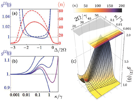
Figure 2: (color online) (a) The second-order phonon-phonon correlation function $g^{(2)}(0)$ (blue lines) and the mean phonon number in the cavity $\langle n\rangle$ (red curves) as a function of the QD-laser detuning $\Delta$ normalized by the Rabi frequency $2\Omega$ and beyond the secular approximation (continuous lines), and within the secular approximation (dashed curves). Here $\bar{n}=0.04$, $2\Omega/\gamma=25$ and $\kappa/\gamma=5\times 10^{-3}$. (b) $g^{(2)}(0)$ as a function of the normalized damping rate $\kappa/\gamma$ for thermal baths at different temperatures and for $2\Omega/\gamma=25$, and $\Delta/(2\Omega)=-0.7$. Here, from top to down one has $\bar{n}=0.64$, $\bar{n}=0.16$, $\bar{n}=0.08$, $\bar{n}=0.04$ and $\bar{n}=0.01$, respectively. (c) $g^{(2)}(0)$ (3D surface) and $\langle n\rangle$ (density plot) as functions of $\kappa/\gamma$ and $2\Omega/\gamma$. Here $\bar{n}=0.04$ whereas $\Delta/(2\Omega)=-0.7$. The plot regions corresponding to $g^{(2)}(0)>1$ and $g^{(2)}(0)<1$ are represented in different mesh styles. The plot region corresponding to $\langle n\rangle<1$ is represented in gray color. The purple curves in figures (b) and (c) are identical. Other parameters are: $\gamma_{c}/\gamma=0.1$, $g/\gamma=15$, $\omega_{ph}/\gamma=35$.

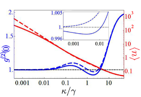
Figure 3: (color online) The second-order phonon-phonon correlation function $g^{(2)}(0)$ (blue lines) and the mean phonon number in the cavity mode $\langle n\rangle$ (red curves) as a function of the cavity damping rate $\kappa$ normalized by the spontaneous emission rate $\gamma$. The continuous curves are beyond the secular approximation whereas the dashed ones are within the secular approximation. Here, $2\Omega/\gamma=25$, $\Delta/(2\Omega)=-0.7$, $\bar{n}=0.04$, $\gamma_{c}/\gamma=0.1$, $g/\gamma=15$ and $\omega_{ph}/\gamma=35$. The continuous blue line is identical with the purple lines of Fig. (2). The inset picture represents a close look on the behaviors of the second-order correlation functions in the regions around $10^{-3}\leq\kappa/\gamma\leq 10^{-2}$.

III Results and Discussion

Consequently, the average phonon number in the cavity mode is expressed as:

$$\langle n\rangle = \langle b^{\dagger}b\rangle=\sum_{n=0}^{\infty}nP_{n}^{(1)}.$$ (17)

The nanocavity second-order phonon-phonon correlation function is defined as usual glau ,

$$g^{(2)}(0) = \frac{\langle b^{\dagger}b^{\dagger}bb\rangle}{\langle b^{\dagger}b\rangle^{2}}=\frac{\sum_{n=0}^{\infty}n(n-1)P_{n}^{(1)}}{\langle n\rangle^{2}}.$$ (18)

The system of Eqs. (11) - (16) as well as the infinite series in the expressions (17) - (18) must be truncated at a particular value of $n=N_{max}$ such that the variables of interest remain unchanged if one further increases $N_{max}$ ginz .

In what follows, we shall study the system in the steady-state regime, i.e., $\dot{P}_{n}^{(i)}=0$ for $\{i=1\cdots 6\}$. The second-order correlation function given by Eq. (18) and the average phonon number in Eq. (17) are used to describe the phonon field behaviors in the acoustical cavity mode glau . Once truncated, the system of coupled equations (11) - (16) is solved by setting the model’s parameters $\{\gamma,\gamma_{c},g,\omega_{ph},\kappa,\bar{n},\Omega\}$ and $\Delta$, respectively.

A general overview over the steady-state system’s behavior in the strong coupling regime or within the secular approximation, i.e. when $\{\bar{\Delta},\bar{\beta}=0\}$, is presented in Fig. 2. The phonon field’s statistics is described by the second-order correlation function $g^{(2)}(0)$ with $g^{(2)}(0)=1$ describing the Poissonian phonon distribution while when $g^{(2)}(0)<1$ one has sub-Poissonian phonon statistics. One observes that moderate laser-QD coupling strengths, i.e. $\Omega$, as well as lower temperatures give a more prominent sub-Poissonian phonon statistics. Furthermore, beyond the secular approximation, the phonon statistics exhibits quantum features, i.e. $g^{(2)}(0)<1$ (compare the corresponding curves in Fig. 2a) and the effect is more pronounced for stronger QD-phonon coupling strengths. Fig. 2(b) shows, beyond the secular approximation, the second-order phonon-phonon correlation function as a function of $\kappa/\gamma$. Here, again, around $\kappa>\gamma$ one has a quantum phonon effect, i.e. sub-Poissonian phonon statistics. Thus, the contribution to the system’s dynamics of the fast rotating terms $H_{fast}^{eff}$ evaluated by the Eq. (5) are essential for a sub-Poissonian quantum feature, see Fig. 2. In Fig. 3 we compare our result within and beyond the secular approximation. The second-order correlation function estimated in both cases converges for higher and smaller cavity damping rates. However, for lower values of $\kappa/\gamma$ quantum features are proper only beyond the secular approximation (see the inset picture in Fig. 3). Furthermore, the mean phonon number decreases in this particular case although it is quite high comparing to the $\kappa>\gamma$ situation.

IV Summary

In summary, we have investigated the phonon quantum statistics in an acoustical nanocavity. A laser-pumped two-level quantum dot is embedded in the cavity contributing to phonon quantum dynamics. We have demonstrated that stronger QD-phonon-cavity coupling regimes lead to quantum features of the cavity phonon field in the steady-state. This QD-cavity interaction regime obliges to go beyond the secular approximation. Ignoring this fact would lead to an erroneous estimation of the phonon statistics for some parameter domains.

References

• (1) G. Rempe, F. Schmidt-Kaler, H. Walther, Phys. Rev. Lett. 64, 2783 (1990).
• (2) C.-S. Chuu, F. Schreck, T. P. Meyrath, J. L. Hanssen, G. N. Price, M. G. Raizen, Phys. Rev. Lett. 95, 260403 (2005).
• (3) Th. Jacqmin, J. Armijo, T. Berrada, K. V. Kheruntsyan, I. Bouchoule, Phys. Rev. Lett. 106, 230405 (2011).
• (4) T. Rocheleau, T. Ndukum, C. Macklin, J. B. Hertzberg, A. A. Clerk, K. C. Schwab, Nature (London) 463, 72 (2010).
• (5) A.D. O’Connell, M. Hofheinz, M. Ansmann, Radoslaw C. Bialczak, M. Lenander, E. Lucero, M. Neeley, D. Sank, H. Wang, M. Weides, J. Wenner, J. M. Martinis, A. N. Cleland, Nature (London) 464, 697 (2010).
• (6) J. Chan, T. P. Mayer Alegre, A. H. Safavi-Naeini, J. T. Hill, A. Krause, S. Gröblacher, M. Aspelmeyer, O. Painter, Nature (London) 478, 89 (2011).
• (7) W. Kütt, W. Albrecht, H. Kurz, IEEE J. Quantum Electron. 28, 2434-2444 (1992).
• (8) A. Bartels, Th. Dekorsy, H. Kurz, Phys. Rev. Lett. 82, 1044 (1999).
• (9) Y. Ezzahri, S. Grauby, J. M. Rampnoux, H. Michel, G. Pernot, W. Claeys, S. Dilhaire, C. Rossignol, G. Zeng, A. Shakouri, Phys. Rev. B 75, 195309 (2007).
• (10) I. Mahboob, K. Nishiguchi, A. Fujiwara, H. Yamaguchi, Phys. Rev. Lett. 110, 127202 (2013).
• (11) I. S. Grudinin, H. Lee, O. Painter, K. J. Vahala, Phys. Rev. Lett. 104, 083901 (2010).
• (12) K. Vahala, M. Hermann, S. Knünz, V. Batteiger, G. Saathoff, T. W. Hänsch, Th. Udem, Nat. Phys. 5, 682 (2009).
• (13) H. Jing, S. K. Özdemir, Xin-You Lü, J. Zhang, L. Yang, F. Nori, Phys. Rev. Lett. 113, 053604 (2014).
• (14) H. Wang, Z. Wang, J. Zhang, S. K. Özdemir, L. Yang, Yu-xi Liu, Phys. Rev. A 90, 053814 (2014).
• (15) H. Wu, G. Heinrich, F. Marquardt, New J. Phys. 15, 123022 (2013).
• (16) J. Kabuss, A. Carmele, T. Brandes, A. Knorr, Phys. Rev. Lett. 109, 054301 (2012).
• (17) J. Kabuss, A. Carmele, A. Knorr, Phys. Rev. B 88, 064305 (2013).
• (18) R. Okuyama, M. Eto, T. Brandes, New J. Phys. 15, 083032 (2013).
• (19) A. B. Bhattacherjee, T. Brandes, Can. J. Phys. 91, 639 (2013).
• (20) T. Figueiredo Roque, A. Vidiella-Barranco, arXiv: 1406.1987v3 [quant-ph] (2014).
• (21) P. D. Nation, Phys. Rev. A 88, 053828 (2013).
• (22) M. Merlo, F. Haupt, F. Cavaliere, M. Sassetti, New J. Phys. 10, 023008 (2008).
• (23) A. Kronwald, F. Marquardt, A. A. Clerk, Phys. Rev. A 88, 063833 (2013).
• (24) J. Qian, A. A. Clerk, K. Hammerer, F. Marquardt, Phys. Rev. Lett. 109, 253601 (2012).
• (25) M. Aspelmeyer, T. J. Kippenberg, F. Marquardt, Rev. Mod. Phys. 86, 1391 (2014).
• (26) M. Trigo, A. Bruchhausen, A. Fainstein, B. Jusserand, V. Thierry-Mieg, Phys. Rev. Lett. 89, 227402 (2002).
• (27) N. D. Lanzillotti-Kimura, A. Fainstein, B. Perrin, B. Jusserand, L. Largeau, O. Mauguin, A. Lemaitre, Phys. Rev. B 83, 201103 (2011).
• (28) Ö. O. Soykal, R. Ruskov, Ch. Tahan, Phys. Rev. Lett. 107, 235502 (2011).
• (29) H. Kim, Th. C. Shen, K. Roy-Choudhury, G. S. Solomon, E. Waks, Phys. Rev. Lett. 113, 027403 (2014).
• (30) M. Scully, M. S. Zubairy, Quantum Optics (Cambridge University Press, Cambridge, 1997).
• (31) M. Kiffner, M. Macovei, J. Evers, and C. H. Keitel, Progress in Optics 55, 85 (2010).
• (32) D. F. V. James, Fortschr. Phys. 48, 823 (2000).
• (33) R. Tan, G.-x. Li, Z. Ficek, Phys. Rev. A 78, 023833 (2008).
• (34) T. Quang, P. L. Knight, and V. Buzek, Phys. Rev. A 44, 6092 (1991).
• (35) R. J. Glauber, Phys. Rev. 130, 2529 (1963).
• (36) C. Ginzel, H.-J. Briegel, U. Martini, B.-G. Englert, A. Schenzle, Phys. Rev. A 48, 732 (1993).