Maximum group velocity in a one-dimensional model with a sinusoidally varying staggered potential

Abstract

We use Floquet theory to study the maximum value of the stroboscopic group velocity in a one-dimensional tight-binding model subjected to an on-site staggered potential varying sinusoidally in time. The results obtained by numerically diagonalizing the Floquet operator are analyzed using a variety of analytical schemes. In the low frequency limit we use adiabatic theory, while in the high frequency limit the Magnus expansion of the Floquet Hamiltonian turns out to be appropriate. When the magnitude of the staggered potential is much greater or much less than the hopping, we use degenerate Floquet perturbation theory; we find that dynamical localization occurs in the former case when the maximum group velocity vanishes. Finally, starting from an “engineered” initial state where the particles (taken to be hard core bosons) are localized in one part of the chain, we demonstrate that the existence of a maximum stroboscopic group velocity manifests in a light cone like spreading of the particles in real space.

I Introduction

In the real world, the speed at which information can propagate is limited by the speed of light; this results in the light cone effect as postulated by the special theory of relativity. Is there a similar upper bound of the speed at which correlations (information) can propagate in interacting quantum many-body systems? Following the seminal work by Lieb and Robinson lieb72 , which established the existence of a maximum group velocity in a one-dimensional spin chain with a finite range interaction, some recent studies have explored this conjecture in several interacting many-body systems; these studies do indeed exhibit an effective light cone that sets a bound on the speed of propagation of correlations. This is reflected for example, in the growth of block entanglement entropy following a quench calabrese05 , or the collapse and revival of the Loschmidt echo stephan11 ; happola12 . The light cone like propagation of quantum correlations has also been observed experimentally by quenching a one-dimensional quantum gas in an optical lattice cheneau12 .

In parallel, there have been a plethora of studies of closed quantum systems driven periodically in time in the context of defect productions mukherjee08 ; mukherjee09 , dynamical freezing das10 , dynamical saturation russomanno12 and localization alessio13 ; bukov14 ; nag14 , dynamical fidelity sharma14 , and thermalization lazarides14 (for a review see Ref. dutta15, ). The study of periodically perturbed many-body systems has also gained importance because of the proposal of Floquet (irradiated) graphene gu11 ; kitagawa11 ; morell12 , Floquet topological insulators and the generation of topologically protected edge states kitagawa10 ; lindner11 ; jiang11 ; trif12 ; gomez12 ; dora12 ; cayssol13 ; liu13 ; tong13 ; rudner13 ; katan13 ; lindner13 ; kundu13 ; basti13 ; schmidt13 ; reynoso13 ; wu13 ; manisha13 ; perez1 ; perez2 ; perez3 ; reichl14 ; manisha14 some of which have been experimentally studied kitagawa12 ; rechtsman13 ; puentes14 .

In this work, we use Floquet theory to explore the stroboscopic (i.e., measured at the end of each complete period) group velocity of a system of hard core bosons residing on a one-dimensional lattice in the presence of a staggered potential which is varying sinusoidally in time shirley65 ; griffoni98 . In particular we study the maximum value of the group velocity to observe the consequent light cone effect. Although the time-independent version of the model is integrable, the periodic sinusoidal perturbation renders the situation rather complicated since the corresponding Floquet operator cannot be obtained in a closed analytical form unlike the case of periodic perturbations which are piece-wise continuous in time nag14 ; dasgupta14 . One therefore has to use various approximation schemes valid in the appropriate regions of the parameter space to analyze the behavior of the stroboscopic group velocity.

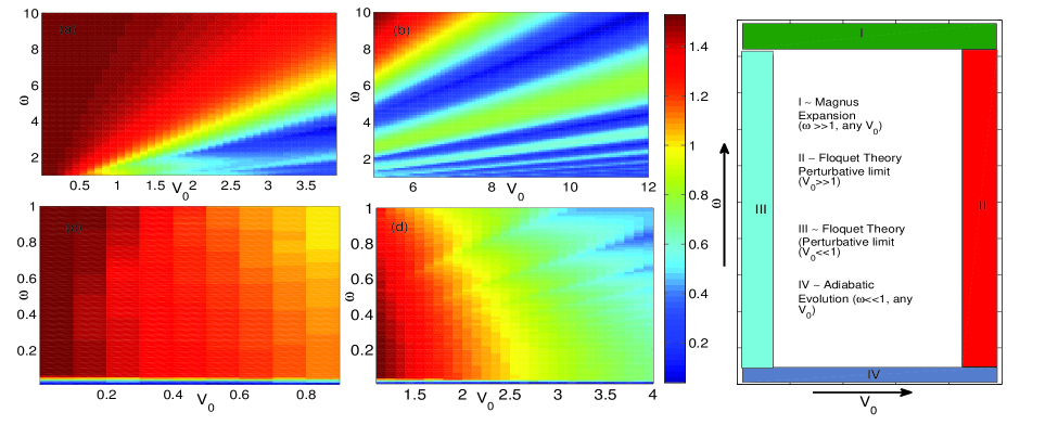
Figure 1: (Color online) Density plots showing the variation of the maximum value of the stroboscopic group velocity as a function of the driving frequency $\omega$ and the magnitude of the sinusoidally varying staggered potential $V_{0}$ (both in units of $\gamma=1$). In (a) $V_{\rm max}$ is always finite (red region) for large $\omega$ and small $V_{0}$ (top left corner). But there are some regions where $V_{\rm max}$ becomes very small (blue region) in the intermediate $\omega$ range and for large $V_{0}$ (bottom right corner). (b) shows that there exists an array of regions where $V_{\rm max}$ vanishes (dark blue regions). The line-like regions of zero velocity are not equispaced in $\omega$ for a given value of $V_{0}$. (c) shows that $V_{\rm max}$ never becomes zero for small $\omega$ and small $V_{0}$, although $V_{\rm max}$ is very small for extremely low frequencies (blue region near the horizontal axis). (d) shows that $V_{\rm max}$ decreases as one increases $V_{0}$ while keeping $\omega$ fixed at small values. At extremely small frequencies, $V_{\rm max}$ shows behavior similar to that in (c). (e) A schematic diagram showing the validity of the various limits of the Floquet theory in different regions in the $\omega-V_{0}$ plane.

The paper is organized in the following way. In Sec. II, we present the Hamiltonian of the model under consideration and discuss the generic behavior of the maximum value of the stroboscopic group velocity $V_{\rm max}$ as a function of the amplitude and frequency of the periodic perturbation; this is derived using the numerically obtained Floquet quasi-energies. In Sec. III, we use adiabatic theory to find the behavior of $V_{\rm max}$ in the low frequency limit while the high frequency limit is treated within a Magnus expansion in Sec. IV. In Sec. V (Sec. VI), we use a Floquet perturbation theory soori10 when the hopping term is much smaller (greater) than the amplitude of the staggered potential. In the case of a large magnitude of the staggered potential, we point to the situations when the maximum stroboscopic group velocity vanishes resulting in the so-called dynamical localization. We demonstrate a light cone like propagation of particles in real space in Sec. VII. Concluding remarks are presented in Sec. VIII.

II Model and the stroboscopic group velocity

We consider a Hamiltonian of the tight-binding form

$$H=-\gamma\sum_{l=1}^{L}(b_{l}^{\dagger}b_{l+1}+b_{l+1}^{\dagger}b_{l}),$$ (1)

where $\gamma$ is the hopping amplitude, and $b_{l}$ denotes bosonic annihilation operators defined on a one-dimensional lattice satisfying the hard core condition $(b_{l}^{\dagger})^{2}=(b_{l})^{2}=0$. The single particle dispersion is given by $E_{k}=-2\gamma\cos k$. This model describes a system of hard core bosons in a gapless superfluid phase klich07 . (By the Jordan-Wigner transformation lieb61 , this system is equivalent to one with spinless fermions). When the system is perturbed by a spatially alternating potential $V_{l}=(-1)^{l}V_{0}$, a gap opens up in the spectrum for any non-zero value of $V_{0}$ thereby driving it to a gapped Mott insulator phase. Our aim here is to investigate the response of the system subjected to an alternating potential varying sinusoidally in time as $V(t)=V_{0}\sin(\omega t)$. We will analyze the behavior of the stroboscopic group velocity, measured after $n$ complete periods of the driving, and its maximum value $V_{\rm max}$ as a function of the driving frequency $\omega$ and the amplitude $V_{0}$.

In the presence of the alternating potential, the Hamiltonian in Eq. (1) reduces in momentum space to a $2\times 2$ matrix form in terms of the momenta $k$ and $k+\pi$,

$$H_{k}(t)=-2\gamma\cos k~{}\sigma^{z}+V_{0}\sin(\omega t)~{}\sigma^{x},$$ (2)

where $\sigma^{x,z}$ denote pseudo-spin Pauli matrices. Clearly the spectrum is gapless for $V_{0}=0$. We will set $\gamma=1$, Planck’s constant $\hbar=1$ and the lattice spacing equal to 1 in the rest of the paper. Hence $\omega$, $V_{0}$, $k$ and $V_{\rm max}$ (to be defined below) will all be dimensionless.

Using the Jordan-Wigner transformation, the time-independent part of the Hamiltonian can be mapped to a system of spinless fermions on a one-dimensional lattice with a hopping amplitude $\gamma$, while the time-dependent part of the Hamiltonian corresponds to a staggered chemical potential which is sinusoidally driven with a frequency $\omega$. This equivalence between the hard core bosonic and the spinless fermionic models does not hold in higher than one dimension. Nevertheless, in higher dimensions there are non-interacting fermionic models with a sinusoidally driven chemical potential for which the behavior of the stroboscopic group velocity and the dynamical localization is similar to what is reported here.

Defining the time period $T=2\pi/\omega$, the stroboscopic Floquet operator for each momentum mode is given by the unitary operator ${\cal F}_{k}(V_{0},T)={\cal T}\exp\left(-i\int_{0}^{T}dtH_{k}(t)\right)$, where ${\cal T}$ denotes the time-ordering. This operator cannot be computed analytically for a sinusoidal driving. One can however numerically calculate ${\cal F}_{k}$ and find its eigenvalues which take the form $\exp(-i\mu_{k}^{\pm}T)$ where $\mu_{k}^{\pm}=\pm\mu_{k}$ are the quasi-energies. The group velocity can be obtained from the quasi-energies as

$$v_{k}=\partial\mu_{k}/\partial k.$$ (3)

The maximum of $v_{k}$ as a function of $k$ gives the quantity $V_{\rm max}$, which is the main object of interest in this paper. The physical interpretation of the stroboscopic group velocity is that if the quantum correlations are measured only at the end of each complete period, they would appear to propagate with a maximum speed $V_{\rm max}$. This quantity is presented in Fig. 1 as a function of $V_{0}$ and $\omega$.

Upon inspecting the results presented in Fig. 1, one finds that $V_{\rm max}$ tends to saturate at some value for large values of $\omega$ and small or intermediate values of $V_{0}$ ($V_{0}\leq 1$) [see Fig. 1 (a)]. The maximum group velocity shows an interesting behavior when both $V_{0}$ and $\omega$ become large, as shown in Fig. 1 (b). In this limit, one finds that for a given frequency $\omega$, $V_{\rm max}$ vanishes in regular intervals of $V_{0}$. On the other hand, for a given $V_{0}$, the zeros of $V_{\rm max}$ lie in increasing intervals of $\omega$. In this regime $V_{\rm max}$ is given by the zeros of a Bessel function as we will show below. But when $\omega$ is small, $V_{\rm max}$ never becomes zero, although in the limit $\omega\to 0$, $V_{\rm max}$ becomes very small irrespective of $V_{0}$; see the bottom regions of Figs. 1 (c) and (d). The maximum group velocity gradually decreases with $V_{0}$ if one keeps $\omega$ fixed at a lower value, as shown in Fig. 1 (d). In subsequent sections, we will use different analytical methods to analyze the various behaviors described here.

Finally, we note that we will consider the entire Brillouin zone ranging from $k=-\pi/2$ to $k=\pi/2$. The time-dependent part of the Hamiltonian in Eq. (1) is quantum critical and gapless in the thermodynamic limit for the modes with $k=\pm\pi/2$. The minimum frequency scale of the bare tight-binding Hamiltonian (with $\hbar=1$) is determined by the system size ($\sim 1/L$), while the maximum frequency scale appears for the modes $k=0,~{}\pi$ and is equal to $2$ since $E_{k}=-2\cos k$.

III Adiabatic limit of low frequency

The behavior of the quasi-energy can be explained in the low frequency limit where the adiabatic theory holds. We will choose the basis states as the eigenstates of the pseudo-spin operator $\sigma^{z}$, i.e., $(1~{}0)^{T}$ and $(0~{}1)^{T}$. In this limit, the product of the time period $T$ and the Floquet quasi-energies $\mu_{k}^{\pm}$ is equal to the dynamical phase $\epsilon_{k}^{\pm}$ accumulated over a complete time period $T$; this is given by

$$\epsilon_{k}^{\pm}=\pm\int_{0}^{2\pi/\omega}~{}dt~{}\sqrt{4\cos^{2}k+V_{0}^{2}\sin^{2}\omega t}~{}=~{}\pm\left[\frac{2\sqrt{4\cos^{2}k+V_{0}^{2}}}{\omega}~{}E\left(\frac{V_{0}^{2}}{V_{0}^{2}+4\cos^{2}k}\right)+\frac{4\cos k}{\omega}~{}E\left(-\frac{1}{4}V_{0}^{2}\sec^{2}k\right)\right],$$ (4)

where $E(x)$ is the elliptic integral gradshteyn . [We note that the Berry phase term vanishes in this problem since the closed path traced out by the Hamiltonian in (2) as $t$ goes from zero to $T$ is a line in the $x-z$ pseudo-spin space; such a line covers zero solid angle at the origin $(x,y,z)=(0,0,0)$.] Interestingly, the behavior of the quasi-energy can be qualitatively explained up to certain values of $V_{0}$. Let us elaborate on this below.

In the limit $V_{0}\ll 1$ and very small $\omega$, we can use the form of the elliptic functions to reduce Eq. (4) to

$$\epsilon_{k}^{\pm}\simeq\pm\left[\frac{4\pi\cos k}{\omega}+\frac{\pi V_{0}^{2}\sec k}{4\omega}+O(V_{0}^{2})\right].$$ (5)

A quasi-degeneracy occurs when this dynamical phase $\epsilon_{k}^{\pm}=m\pi$. This condition successfully gives the number of quasi-degenerate points along with values of the quasi-degenerate momenta, $k=\pm~{}{\rm arccos}[(m\omega+\sqrt{-4V_{0}^{2}+m^{2}\omega^{2}})/8]$ [see Fig. 2 (a)]. (We note that the critical modes $k=\pm\pi/2$ are always quasi-degenerate.)

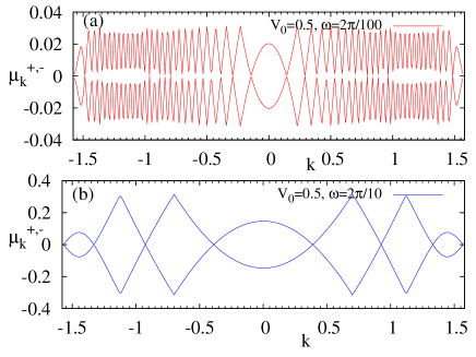
Figure 2: (Color online) Plots showing the variation of the quasi-energy $\mu_{k}^{\pm}$ as a function of $k$ with the potential for $V_{0}<1$. In this parameter regime we choose two cases: (a) $V_{0}>\omega$ and (b) $V_{0}<\omega$. The behavior observed in (a) can be explained using adiabatic theory with small $V_{0}$. The locations of the quasi-degenerate points in (b) are discussed in Sec. VI.

In the intermediate potential range $V_{0}\sim 1$, the behavior of the quasi-energy is again determined by the adiabatic evolution of two-level systems. The number of quasi-degenerate points is successfully given by $\epsilon_{k}^{\pm}=m\pi$, where $\epsilon_{k}^{\pm}$ is given by

$$\epsilon_{k}^{\pm}\simeq\pm\left[\frac{4\cos^{2}k}{V_{0}\omega}+\frac{8\cos^{2}k\log(4V_{0})}{V_{0}\omega}+\frac{4V_{0}}{\omega}\right].$$ (6)

The group velocity can be obtained from Eqs. (5) and (6); in the former case, we find $v_{k}\simeq\pm(2\sin k-(V_{0}^{2}\sec k\tan k)/8+O(V_{0}^{2}))$ while in the latter $v_{k}\simeq\pm(2\sin(2k)/(V_{0}\pi)+4\sin(2k)\log(4V_{0})/(V_{0}\pi))$. Therefore, we conclude that $V_{\rm max}$ is (nearly) independent of $\omega$ for small frequencies; see Fig. 3. We find that $V_{\rm max}=2$ for very small $V_{0}$ while for $V_{0}\gg 1$, $V_{\rm max}\sim 1/V_{0}$ as shown in Fig. 4 for small values of $\omega$. In the limit of small $V_{0}$ and $\omega$ ($\omega<1/L$), the system hardly senses the periodic driving and hence $V_{\rm max}$ is determined by the bare tight-binding Hamiltonian; in the limit of large $V_{0}$, the Floquet perturbation theory holds (see Sec. V) which explains the $1/V_{0}$ decay of $V_{\rm max}$.

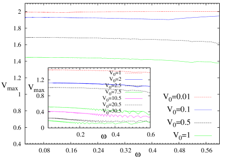
Figure 3: (Color online) Plot showing that the maximum group velocity $V_{\rm max}$ is nearly independent of the frequency (or slightly decreasing with increasing $\omega$) at low frequency for both small and large values of $V_{0}$. $V_{\rm max}$ decreases as $V_{0}$ increases. The inset shows that $V_{\rm max}$ exhibits some wiggles with $\omega$ for high values of $V_{0}$.

IV Magnus expansion for high frequency

The time evolution operator describing the Schrödinger evolution of a quantum system is given by ${\cal T}\exp[-i\int_{0}^{t}dt^{\prime}H(t^{\prime})]=\exp[\Lambda(t)]$. In the Magnus expansion, the operator $\Lambda(t)$ is decomposed in the form $\Lambda(t)=\sum_{k=1}^{\infty}\Lambda_{k}(t)$ blanes09 . The advantage of using a Hamiltonian periodic in time is that the stroboscopic unitary operator (i.e., the Floquet operator) can be expressed in the form $F(T)=\exp(-iH_{F}T)$, where $H_{F}$ is the corresponding Floquet Hamiltonian. Thus, for a periodically driven system, the Magnus expansion enables us to express the Floquet Hamiltonian in the form $H_{F}=\sum_{n=1}^{\infty}H_{F}^{(n)}$, where the $H_{F}^{(n)}$’s can be expressed in the following form alessio13 :

$$H_{F}^{(1)} = \frac{1}{T}\int_{0}^{T}~{}dtH(t),$$

$$H_{F}^{(2)} = -~{}\frac{i}{2T}\int_{0}^{T}~{}dt_{1}~{}\int_{0}^{t_{2}}~{}dt_{2}\left[H(t_{1}),H(t_{2})\right],$$

$$H_{F}^{(3)} = -~{}\frac{1}{6T}\int_{0}^{T}~{}dt_{1}~{}\int_{0}^{t_{2}}~{}dt_{2}\int_{0}^{t_{2}}~{}dt_{3}$$ (7)

$$~{}~{}~{}~{}~{}~{}~{}~{}\left(\left[H(t_{1}),\left[H(t_{2}),H(t_{3})\right]\right]+1\leftrightarrow 3\right).$$

As shown below, the $n$th-order term decreases as $1/\omega^{n-1}$, and is therefore vanishingly small for $\omega\to\infty$. For the model given by Eq. (2), $H_{F,k}^{(1)}=\alpha\sigma^{z}$, $H_{F,k}^{(2)}=2V_{0}\alpha/\omega~{}\sigma^{y}$ and $H_{F,k}^{(3)}=-(4\alpha^{2}V_{0}\pi/3\omega^{2})~{}\sigma^{x}-(3\alpha V_{0}^{2}/\omega^{2})~{}\sigma^{z}$.

We will work in the high frequency limit and retain terms up to the order $1/\omega$. We then arrive at an effective Hamiltonian given by

$$H_{F,k}^{\rm eff}=(\alpha-\frac{3\alpha V_{0}^{2}}{\omega^{2}})~{}\sigma^{z}+\frac{2\alpha V_{0}}{\omega}~{}\sigma^{y}-\frac{4\alpha^{2}V_{0}\pi}{3\omega^{2}}~{}\sigma^{x},$$ (8)

where $\alpha=-2\cos k$. The effective quasi-energies, obtained by diagonalizing (8) and retaining terms of order $(V_{0}/\omega)^{2}$, are found to be $\mu_{\rm eff}^{\pm}=\pm\sqrt{\alpha^{2}-2\alpha^{2}V_{0}^{2}/\omega^{2}}\simeq\pm\alpha(1-V_{0}^{2}/\omega^{2})$; the quasi-degeneracy points occur at $k=\pm\pi/2$ where $\alpha$ vanishes. In the limit $\omega\to\infty$, $\mu_{\rm eff}^{\pm}\approx\pm\alpha$ . Therefore, the maximum group velocity $V_{\rm max}$ becomes $2$ irrespective of $V_{0}$. This can also be explained simply by noting that the periodically varying perturbation in the Hamiltonian (2) vanishes on average in the high frequency limit. Moreover, for smaller values of $V_{0}$, $V_{\rm max}$ reaches its saturation value $V_{\rm max}=2$ at a smaller value of $\omega$ as compared to higher values of $V_{0}$.

V Large potential compared to the hopping amplitude: $V_{0}\gg\gamma$

Let us now examine the case where the hopping amplitude $\gamma$ can be treated as a perturbing parameter in the Hamiltonian given by Eq. (2). It is useful to consider a unitary transformation which shifts the time dependence of the Hamiltonian to the diagonal term, so that the transformed Hamiltonian takes the form $H_{k}(t)=V_{0}\sin(\omega t)\sigma^{z}+2\gamma\cos k\sigma^{x}$. (We now set $\gamma=1$ as usual). The time-dependent Schrödinger equation in the new basis can then be written as $i|\dot{\phi}_{k}^{\pm}(t)\rangle=H_{k}(t)|\phi_{k}^{\pm}(t)\rangle$. Dividing both sides of the equation by $V_{0}$ and rescaling $t$ to $tV_{0}$, the Schrödinger equation can be rewritten as

$$i|\dot{\phi}^{+}_{k}(t)\rangle = \sin(\frac{\omega}{V_{0}}t)|\phi^{+}_{k}(t)\rangle+\frac{2\cos k}{V_{0}}|\phi^{-}_{k}(t)\rangle,$$

$$i|\dot{\phi}^{-}_{k}(t)\rangle = -\sin(\frac{\omega}{V_{0}}t)|\phi^{-}_{k}(t)\rangle+\frac{2\cos k}{V_{0}}|\phi^{+}_{k}(t)\rangle.$$ (9)

We will set $\omega/V_{0}=a$ and $2\cos k/V_{0}=b$ in subsequent calculations. The solutions in the zeroth order of $w$ are given by

$$|\phi_{k}^{+}(t)\rangle = \left(\begin{array}[]{cc}c_{k}^{+}(0)~{}e^{i\cos(at)/a}\\ 0\end{array}\right),$$ (12)

$$|\phi_{k}^{-}(t)\rangle = \left(\begin{array}[]{cc}0\\ c_{k}^{-}(0)~{}e^{-i\cos(at)/a}\end{array}\right),$$ (15)

where $c_{k}^{\pm}(0)$ denote the probability amplitudes of the states $|\phi_{k}^{\pm}\rangle$ at time $t=0$. We find that $|\phi_{k}^{+}(T)\rangle=|\phi_{k}^{+}(0)\rangle$ and $|\phi_{k}^{-}(T)\rangle=|\phi_{k}^{-}(0)\rangle$, implying that these solutions are degenerate in Floquet theory. We therefore employ a degenerate perturbation theory to include the hopping term perturbatively and find the time-dependent coefficients $c_{k}^{\pm}(t)$, which satisfy the evolution equations

$$i\dot{c}_{k}^{+}(t) = bc_{k}^{-}(t)~{}e^{-i2\cos(at)/a},$$

$$i\dot{c}_{k}^{-}(t) = bc_{k}^{+}(t)~{}e^{i2\cos(at)/a}.$$ (16)

To incorporate the correction up to first order in the hopping, we substitute $c_{k}^{\pm}(t)$ appearing on the right sides of Eqs. (16) by $c_{k}^{\pm}(0)$, respectively. The solution at time $t=T=2\pi/a$ is then given by

$$c_{k}^{+}(T) = c_{k}^{+}(0)-(i2\pi bc_{k}^{-}(0)/a)~{}J_{0}(2V_{0}/\omega),$$

$$c_{k}^{-}(T) = c_{k}^{-}(0)-(i2\pi bc_{k}^{+}(0)/a)~{}J_{0}(2V_{0}/\omega).$$ (17)

Up to first order in the hopping $\gamma$, the Floquet operator is given by

$$F_{k}(T)=\left[\begin{array}[]{cc}1&-(i2\pi b/a)J_{0}(2V_{0}/\omega)\\ -(i2\pi b/a)J_{0}(2V_{0}/\omega)&1\end{array}\right],$$ (18)

so that $(c_{k}^{+}(T)~{}c_{k}^{-}(T))^{T}=F_{k}(T)(c_{k}^{+}(0)~{}c_{k}^{-}(0))^{T}=\exp(i\theta_{k}^{\pm})(c_{k}^{+}(0)~{}c_{k}^{-}(0))^{T}$, where $(...~{}...)^{T}$ denotes transpose. Diagonalizing matrix (18), one obtains the eigenvalues $e^{i\theta_{k}^{\pm}}$, and hence $\theta_{k}^{\pm}=\mu_{k}^{\pm}T=\pm(2\pi b/a)~{}J_{0}(2V_{0}/\omega)=2\cos kJ_{0}(2V_{0}/\omega)$.

For large $V_{0}$ and large $\omega$, the quasi-energy is given by $\mu_{k}^{\pm}\simeq\pm 2\cos k\sqrt{\omega/\pi V_{0}}\cos(2V_{0}/\omega-\pi/4)$. The maximum group velocity is $V_{\max}=2\sqrt{\omega/\pi V_{0}}\cos(2V_{0}/\omega-\pi/4)$ which that vanishes at $2V_{0}/\omega=(n+3/4)\pi$. This matches the observed numerical results presented in Fig. 4. We note that the maximum group velocity vanishes when $J_{0}(2V_{0}/\omega)=0$.

Furthermore, given $\mu_{k}^{\pm}=\pm 2\cos kJ_{0}(2V_{0}/\omega)$, one can find the values of the momenta for which quasi-degeneracies occur in the Floquet spectrum given by $\mu_{k}T=m\pi$, namely, $k={\rm arccos}[m\omega/(4J_{0}(2V_{0}/\omega))]$. A solution for $k=\pm\pi/2$ can be found only for $m=0$. This behavior is identical to that obtained from the Magnus expansion for $\omega\gg V_{0}$. From Fig. 4, we find that for high $V_{0}$, Floquet perturbation theory works better at higher frequencies where $V_{\rm max}=2J_{0}(2V_{0}/\omega)$. We note that for very small values of $\omega$, $V_{\rm max}$ falls off as $1/V_{0}$ as predicted by the adiabatic theory. Therefore, a crossover in the behavior of $V_{\rm max}$ as a function of $V_{0}$ and $\omega$ is expected. The crossover happens between two types of behaviors of the maximum group velocity, i.e., $V_{\rm max}\propto V_{0}^{-1}$ and $V_{\rm max}\propto 2J_{0}(2V_{0}/\omega)$. Although $V_{\rm max}$ never becomes zero (but shows a dip) at the zeros of a Bessel function for small $\omega$, we find that $V_{\rm max}$ indeed vanishes at these points for higher values of $\omega$.

The vanishing of $V_{\rm max}$ when $J_{0}(2V_{0}/\omega_{0})=0$, corresponds to the coherent destruction of tunneling grossmann91 ; kayanuma94 or dynamical freezing das10 . When the bare energies (diagonal terms) of a two-level system are sinusoidally driven with a driving frequency which is much larger than the tunneling (appearing in the off-diagonal terms of the corresponding $2\times 2$ Hamiltonian), the system may get frozen in its initial state even though the dynamics is perfectly unitary; this is known as the coherent destruction of tunneling which occurs when the transition probability to the other state given by $J_{0}(2V_{0}/\omega_{0})$ vanishes. The present model ideally represents such a situation when $V_{0}\gg 1$ and $\omega_{0}\gg 1$ with $V_{0}/\omega_{0}\sim O(1)$ as also observed numerically in Fig. 4. Whenever $V_{\rm max}$ vanishes, the quantum correlations do not propagate as we will discuss in Sec. VII; this also leads to a real space localization of hard core bosons.

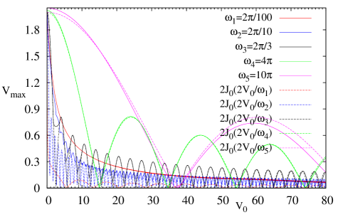
Figure 4: (Color online) Variation of the maximum group velocity as a function of $V_{0}$. For higher values of $V_{0}$ and frequency $\omega$, the numerically obtained $V_{\rm max}$ is found to match the Bessel function given by $2~{}J_{0}(2V_{0}/\omega)$. On the other hand, for very small values of the frequency $V_{\rm max}$ does not match the Bessel function.

VI Small potential compared to the hopping amplitude: $V_{0}\ll\gamma$

We now consider the other limit, $V_{0}\ll\gamma=1$, when $V_{0}$ can be treated perturbatively. At the zeroth order in $V_{0}$, the Hamiltonian (2) reduces to $H_{k}=-2\cos k~{}\sigma^{z}$ with eigenfunctions

$$|\phi_{k}^{+}(t)\rangle=\left(\begin{array}[]{cc}e^{-i2\cos k~{}t}\\ 0\end{array}\right),~{}~{}~{}|\phi_{k}^{-}(t)\rangle=\left(\begin{array}[]{cc}0\\ ~{}e^{i2\cos k~{}t}\end{array}\right).$$ (19)

In the non-degenerate case when $e^{-i2\cos k~{}T}\neq e^{i2\cos k~{}T}$, $T=2\pi/\omega$, it can be easily shown that the first order correction in the quasi-energy vanishes since $\langle\sigma^{x}\rangle=0$ when the expectation values are calculated with the eigenfunctions in Eq. (19). This necessitates the application of a degenerate perturbation theory soori10 when the condition $e^{-i2\cos k~{}T}=\pm 1$ is satisfied, implying that $4\cos k=m\omega$. We will distinguish between two situations, $4\cos k/\omega\neq 1$ and $4\cos k/\omega=1$; as we will show below, in the former case there is a correction of order $V_{0}^{2}$, while in the latter case a correction of order $V_{0}$ emerges.

Let us first discuss the situation in which $4\cos k/\omega\neq 1$. In the same spirit as in Sec. V, the quasi-states are chosen to be

$$|\phi_{k}^{+}(t)\rangle = \left(\begin{array}[]{cc}c_{k}^{+}(t)~{}e^{-i2\cos k~{}t}\\ 0\end{array}\right),$$ (22)

$$|\phi_{k}^{-}(t)\rangle = \left(\begin{array}[]{cc}0\\ c_{k}^{-}(t)~{}e^{i2\cos k~{}t}\end{array}\right).$$ (25)

We note that $|\phi_{k}^{+}(T)\rangle=e^{-i2T\cos k}|\phi_{k}^{+}(0)\rangle$ and $|\phi_{k}^{-}(T)\rangle=e^{i2T\cos k}|\phi_{k}^{-}(0)\rangle$. The time-dependent coefficients satisfy the Schrödinger equation

$$i\dot{c}_{k}^{+}(t) = -iV_{0}\sin(\omega t)~{}c_{k}^{-}(t)~{}e^{-i4t\cos k},$$

$$i\dot{c}_{k}^{-}(t) = -iV_{0}\sin(\omega t)~{}c_{k}^{+}(t)~{}e^{i4t\cos k}.$$ (26)

Within the first order perturbative approximation, we substitute $c_{k}^{\pm}(t)=c_{k}^{\pm}(0)$ on the right hand side of the above equations. At $t=T$, we find that

$$c_{k}^{+}(T) = c_{k}^{+}(0)-\frac{\omega V_{0}c_{k}^{-}(0)}{\omega^{2}-16\cos^{2}k}\sin(4T\cos k),$$

$$c_{k}^{-}(T) = c_{k}^{-}(0)+\frac{\omega V_{0}c_{k}^{+}(0)}{\omega^{2}-16\cos^{2}k}\sin(4T\cos k).$$ (27)

Considering first the situation $4\cos k\neq\omega$, the Floquet operator up to the first order in $V_{0}$ at time $t=T$ is given by

$$F_{k}(T)=\left[\begin{array}[]{cc}e^{-i2T\cos k}&-\frac{\omega V_{0}}{\omega^{2}-16\cos^{2}k}\sin(4T\cos k)e^{-i2T\cos k}\\ \frac{\omega V_{0}}{\omega^{2}-16\cos^{2}k}\sin(4T\cos k)e^{i2T\cos k}&e^{i2T\cos k}\end{array}\right].$$ (28)

Diagonalizing the Floquet operator in Eq. (28), we get the Floquet quasi-energies $\exp(i\mu_{k}^{\pm}T)=\cos(2T\cos k)\pm i\sqrt{\sin^{2}(2T\cos k)+[\omega V_{0}\sin(4T\cos k)/(\omega^{2}-16\cos^{2}k)]^{2}}$, and hence $\mu_{k}^{\pm}=2\cos k+O(V_{0}^{2})$. The maximum group velocity becomes equal to $2$ for small $V_{0}$.

On the other hand, when $4\cos k=\omega$, we have $|\phi_{k}^{+}(T)\rangle=|\phi_{k}^{+}(0)\rangle$ and $|\phi_{k}^{-}(T)\rangle=|\phi_{k}^{-}(0)\rangle$ to zeroth order in $V_{0}$. Solving the Schrödinger equations within the first order approximation, one finds that the time-dependent coefficients are given by

$$c_{k}^{+}(T)=c_{k}^{+}(0)+\frac{\pi V_{0}c_{k}^{-}(0)}{\omega},~{}~{}c_{k}^{-}(T)=c_{k}^{-}(0)-\frac{\pi V_{0}c_{k}^{+}(0)}{\omega}.$$ (29)

The Floquet operator is given by

$$F_{k}(T)=\left[\begin{array}[]{cc}1&V_{0}\pi/\omega\\ -V_{0}\pi/\omega&1\end{array}\right].$$ (30)

The eigenvalues of the Floquet operator are $e^{i\mu_{k}^{\pm}T}=1\pm iV_{0}\pi/\omega$. The quasi-energy $\mu_{k}^{\pm}={\log}(1\pm iV_{0}\pi/\omega)/T\approx\pm V_{0}/2$, leading to a first-order correction to the quasi-energy unlike the previous case $4\cos k\neq\omega$. We also find that the quasi-degenerate momentum modes are given by $k=\pm~{}{\rm arccos}(m\omega/4)$. Referring to Fig. 2 (b) for $V_{0}=0.5$ and $\omega=2\pi/10$, we note that the number of quasi-degenerate points is successfully predicted by this theory. A correction to the quasi-energy of the order of $V_{0}$ appears at only $m=1$.

VII Light cone like propagation of particles in real space with stroboscopic time $T$

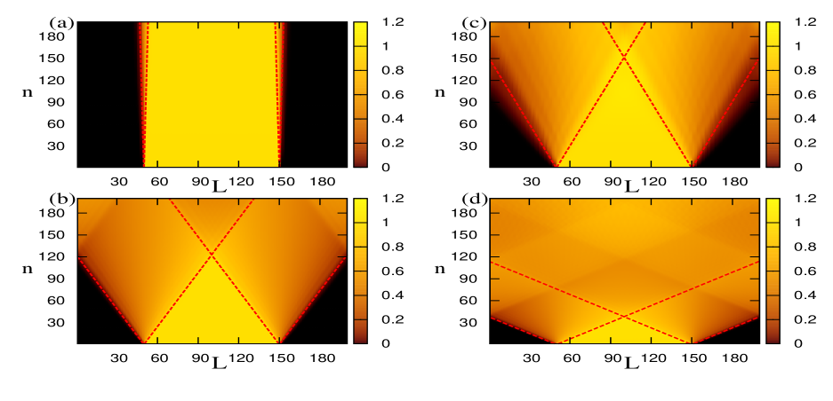
Figure 5: (Color online) Density of particles as a function of the stroboscopic time $nT$ and lattice site $L$. The red dotted line signifies the localization-delocalization boundary. One can determine the maximum group velocity from the slope of this line [$V_{\rm max}=dL/(Tdn)$], which is found to agree well with $V_{\rm max}$ obtained analytically from a Bessel function. Fig. (a) depicts a situation where a dynamical localization (dynamical freezing) nearly happens, for $\omega=4\pi$ and $V_{0}=15$; $V_{\rm max}$ nearly vanishes when $J_{0}(2V_{0}/\omega)=0$. (b) shows that particles move with a maximum group velocity of $V_{\rm max}=0.814$ for $\omega=4\pi$ and $V_{0}=24$. (c) and (d) show that no dynamical localization is observed for $\omega=2\pi/3$ with $V_{0}=12$ and $V_{0}=14$, respectively.

In the earlier sections, we discussed the maximum group velocity $V_{\rm max}$ for a given set of parameter values $V_{0}$ and $\omega$ as presented in Fig. 1. Here we illustrate how the light cone effect arising due to the existence of an upper bound to the group velocity manifests in the real space propagation of particles as shown in Fig. 5; we see that there is a dynamical localization when $V_{\rm max}\to 0$. This is illustrated by choosing an initial state at $t=0$ of a $200$-site system in which the sites labeled $51$ to $150$ are filled (shown by the light region) and the remaining sites are empty (shown by the dark region); this initial state evolves with the total Hamiltonian, i.e., the tight-binding part as well as the sinusoidal driving of the staggered potential. For every stroboscopic instant ($t=nT$), we can find the particle density at each site by numerically studying the time evolution of the initial density matrix $\rho(0)$, namely, $\rho(nT)=F(nT)\rho(0)F^{\dagger}(nT)$, where $F(nT)$ is the real space Floquet operator at time $t=nT$. The slope of the red dotted line separating the occupied and unoccupied regions in Fig. 5 is proportional to $\pm V_{\rm max}$; this clearly demonstrates the light cone like propagation.

The above scenario leads to a couple of important observations. First, when the system is observed stroboscopically one finds a linearly spreading boundary separating the occupied and unoccupied regions. This emphasizes the existence of a $V_{\rm max}$ with which information (in this case, the bosons themselves) can propagate, thereby establishing an equivalent to the Lieb-Robinson limit lieb72 in a sinusoidally driven quantum system which is at a gapless quantum critical point in the absence of the driving term. Second, there can be situations when $V_{\rm max}$ vanishes in the asymptotic limit $n\to\infty$, which corresponds to a real space dynamical localization of the particles; this also implies that the system stops absorbing energy over a complete period even if it is being periodically driven. However, the particles would spread uniformly if the driving is stopped, which leads to the conclusion that this localization is indeed a result of the periodic driving.

Recently, there has been an experimental observation of light cone like spreading of “two-point parity correlation” in an optical lattice under a sudden quenching of the on-site interaction strength from a deep Mott insulating phase to the vicinity of a superfluid-Mott insulator boundary cheneau12 . The existence of an upper bound on the speed has been explained using the notion of the counter-propagation of quasiparticles (“holon” and “doublon”) generated due to the quench. Moreover, a dynamical localization-to-delocalization transition has been observed in a quantum kicked rotator, realized by placing cold atoms in a pulsed, far-detuned, standing wave, by measuring the number of zero velocity atoms under the influence of a quasiperiodic driving ringot00 . In connection to our work, the dynamical localization we predict can be experimentally observed by realizing the hard core boson model in an optical lattice with a sinusoidally varying alternating on-site potential and measuring the current stroboscopically starting from an initial current carrying ground state (obtained by applying a synthetic gauge potential lin09 to the one-dimensional optical lattice). A vanishing current in the large time limit ($t=nT$ with $n\gg 1$) for a particular set of values of $V_{0}$ and $\omega$ would signify the existence of a dynamically localized state. Similarly, the light cone propagation of a wave packet can also be realized by measuring the quasiparticle correlation function with time; the upper bound on the velocity, $V_{\rm max}$, can be determined from the first maximum of the correlation function as a function of time and distance.

VIII Concluding remarks

We have analyzed the behavior of a one-dimensional system of hard core bosons which have a nearest neighbor hopping amplitude $\gamma=1$ and are driven by a sinusoidally varying staggered potential with magnitude $V_{0}$ and frequency $\omega$. We have derived the maximum group velocity $V_{\rm max}$ from the quasi-energies computed numerically from the Floquet operator. A number of analytical approximation methods have been used to study $V_{\rm max}$ in different regions in the parameter space. Within the adiabatic approximation (which is valid when $\omega\to 0$), we find that $V_{\rm max}$ is independent of $\omega$ for small $V_{0}$ and scales as $1/V_{0}$ for large $V_{0}$. For large frequencies we use the Magnus expansion of the Floquet Hamiltonian and find that $V_{\rm max}=2$, independent of the magnitude of $V_{0}$. In this limit, the periodic perturbation vanishes on average and only the tight-binding part of the Hamiltonian contributes to the group velocity. In the limit $V_{0}\gg\gamma$, we show that the Floquet perturbation theory correctly predicts the vanishing of $V_{\rm max}$ for $J_{0}(2V_{0}/\omega)=0$; this dynamical localization is particularly prominent in the limit of large $V_{0}$ and $\omega$ with $V_{0}/\omega\sim 1$. In the other limit $V_{0}\ll\gamma$, there is a correction to the group velocity at first order in $V_{0}$ when the condition $4\gamma\cos k=m\omega$ is satisfied.

Finally, starting from an initial state where the hard core bosons are localized in one part of the chain, we demonstrate that the existence of $V_{\rm max}$ sets an upper bound on the speed with which particles propagate leading to a light cone like spreading of the particles in real space. The dynamically localized (or frozen) phase is characterized by a vanishing $V_{\rm max}$.

None of the analytical methods work in the intermediate region when $V_{0}$ and $\omega$ are both of the order of $\gamma$ (shown by the central region in the right panel of Fig. 1). An analysis of the behavior of $V_{\rm max}$ in this region may be an interesting subject for future research.

We conclude with the remark that the result presented here for a sinusoidal driving is not special to a one-dimensional model of hard core bosons (which is equivalent to a fermionic model in one dimension). A similar behavior of the stroboscopic group velocity, especially the dynamical localization, can be shown to occur in models with non-interacting fermions on a variety of higher dimensional hyper-cubic lattices.

References

- (1)
- (2) E. H. Lieb and D. W. Robinson, Commun. Math. Phys. 28, 251 (1972).
- (3) P. Calabrese and J. Cardy, J. Stat. Mech. (2005) P04010.
- (4) J.-M. Stephan and J. Dubail, J. Stat. Mech. (2011) P08019.
- (5) J. Happola, G. B. Halasz, and A. Hamma, Phys. Rev. A 85, 032114 (2012).
- (6) M. Cheneau, P. Barmettler, D. Poletti, M. Endres, P. Schauß, T. Fukuhara, C. Gross, I. Bloch, C. Kollath, and S. Kuhr, Nature (London) 1481, 484 (2012).
- (7) V. Mukherjee, A. Dutta, and D. Sen, Phys. Rev. B 77, 214427 (2008).
- (8) V. Mukherjee and A. Dutta, J. Stat. Mech (2009) P05005.
- (9) A. Das, Phys. Rev. B 82, 172402 (2010).
- (10) A. Russomanno, A. Silva, and G. E. Santoro, Phys. Rev. Lett. 109, 257201 (2012).
- (11) L. D’Alessio and A. Polkovnikov, Ann. Phys. (N.Y.) 333, 19 (2013).
- (12) M. Bukov, L. D’Alessio, and A. Polkovnikov, arXiv:1407.4803v3.
- (13) T. Nag, S. Roy, A. Dutta, and D. Sen, Phys. Rev. B 89, 165425 (2014).
- (14) S. Sharma, A. Russomanno, G. E. Santoro, and A. Dutta, EPL 106, 67003 (2014).
- (15) A. Lazarides, A. Das, and R. Moessner, Phys. Rev. Lett. 112, 150401 (2014).
- (16) A. Dutta, G. Aeppli, B. K. Chakrabarti, U. Divakaran, T. Rosenbaum and D. Sen, Quantum Phase Transitions in Transverse Field Spin Models: From Statistical Physics to Quantum Information (Cambridge University Press, Cambridge, 2015).
- (17) Z. Gu, H. A. Fertig, D. P. Arovas, and A. Auerbach, Phys. Rev. Lett. 107, 216601 (2011).
- (18) T. Kitagawa, T. Oka, A. Brataas, L. Fu, and E. Demler, Phys. Rev. B 84, 235108 (2011).
- (19) E. Suárez Morell and L. E. F. Foa Torres, Phys. Rev. B 86, 125449 (2012).
- (20) T. Kitagawa, E. Berg, M. Rudner, and E. Demler, Phys. Rev. B 82, 235114 (2010).
- (21) N. H. Lindner, G. Refael, and V. Galitski, Nature Phys. 7, 490 (2011).
- (22) L. Jiang, T. Kitagawa, J. Alicea, A. R. Akhmerov, D. Pekker, G. Refael, J. I. Cirac, E. Demler, M. D. Lukin, and P. Zoller, Phys. Rev. Lett. 106, 220402 (2011).
- (23) M. Trif and Y. Tserkovnyak, Phys. Rev. Lett. 109, 257002 (2012).
- (24) A. Gomez-Leon and G. Platero, Phys. Rev. B 86, 115318 (2012); Phys. Rev. Lett. 110, 200403 (2013).
- (25) B. Dóra, J. Cayssol, F. Simon, and R. Moessner, Phys. Rev. Lett. 108, 056602 (2012).
- (26) J. Cayssol, B. Dora, F. Simon, and R. Moessner, Phys. Status Solidi RRL 7, 101 (2013).
- (27) D. E. Liu, A. Levchenko, and H. U. Baranger, Phys. Rev. Lett. 111, 047002 (2013).
- (28) Q.-J. Tong, J.-H. An, J. Gong, H.-G. Luo, and C. H. Oh, Phys. Rev. B 87, 201109(R) (2013).
- (29) M. S. Rudner, N. H. Lindner, E. Berg, and M. Levin, Phys. Rev. X 3, 031005 (2013).
- (30) Y. T. Katan and D. Podolsky, Phys. Rev. Lett. 110, 016802 (2013).
- (31) N. H. Lindner, D. L. Bergman, G. Refael, and V. Galitski, Phys. Rev. B 87, 235131 (2013).
- (32) A. Kundu and B. Seradjeh, Phys. Rev. Lett. 111, 136402 (2013).
- (33) V. M. Bastidas, C. Emary, G. Schaller, A. Gómez-León, G. Platero, and T. Brandes, arXiv:1302.0781v2.
- (34) T. L. Schmidt, A. Nunnenkamp, and C. Bruder, New J. Phys. 15, 025043 (2013).
- (35) A. A. Reynoso and D. Frustaglia, Phys. Rev. B 87, 115420 (2013).
- (36) C.-C. Wu, J. Sun, F.-J. Huang, Y.-D. Li, and W.-M. Liu, EPL 104, 27004 (2013).
- (37) M. Thakurathi, A. A. Patel, D. Sen, and A. Dutta, Phys. Rev. B 88, 155133 (2013).
- (38) P. M. Perez-Piskunow, G. Usaj, C. A. Balseiro, and L. E. F. Foa Torres, Phys. Rev. B 89, 121401(R) (2014).
- (39) G. Usaj, P. M. Perez-Piskunow, L. E. F. Foa Torres, and C. A. Balseiro, Phys. Rev. B 90, 115423 (2014).
- (40) P. M. Perez-Piskunow, L. E. F. Foa Torres, and G. Usaj, Phys. Rev. A 91, 043625 (2015).
- (41) M. D. Reichl and E. J. Mueller, Phys. Rev. A 89, 063628 (2014).
- (42) M. Thakurathi, K. Sengupta, and D. Sen, Phys. Rev. B 89, 235434 (2014).
- (43) T. Kitagawa, M. A. Broome, A. Fedrizzi, M. S. Rudner, E. Berg, I. Kassal, A. Aspuru-Guzik, E. Demler, and A. G. White, Nat. Commun. 3, 882 (2012).
- (44) M. C. Rechtsman, J. M. Zeuner, Y. Plotnik, Y. Lumer, D. Podolsky, S. Nolte, F. Dreisow, M. Segev, and A. Szameit, Nature (London) 496, 196 (2013); M. C. Rechtsman, Y. Plotnik, J. M. Zeuner, D. Song, Z. Chen, A. Szameit, and M. Segev, Phys. Rev. Lett. 111, 103901 (2013).
- (45) G. Puentes, I. Gerhardt, F. Katzschmann, C. Silberhorn, J. Wrachtrup, and M. Lewenstein , Phys. Rev. Lett. 112, 120502 (2014).
- (46) J. Shirley, Phys. Rev. 138, B979 (1965).
- (47) M. Griffoni and P. Hänggi, Physics Reports 304, 229 (1998).
- (48) S. Dasgupta, U. Bhattacharya, and A. Dutta, Phys. Rev. E 91, 052129 (2015).
- (49) A. Soori and D. Sen, Phys. Rev. B 82, 115432 (2010).
- (50) I. Klich, C. Lannert, and G. Refael, Phys. Rev. Lett. 99, 205303 (2007).
- (51) E. Lieb, T. Schultz, and D. Mattis, Ann. Phys. (N.Y.) 16, 407 (1961).
- (52) I. S. Gradshteyn and I. M. Ryzhik, Table of Integrals, Series, and Products (Academic, London, 2000).
- (53) S. Blanes, F. Casas, J. A. Oteo, and J. Ros, Phys. Rep. 470, 151 (2009).
- (54) F. Grossmann, T. Dittrich, P. Jung, and P. Hänggi, Phys. Rev. Lett. 67, 516 (1991).
- (55) Y. Kayanuma, Phys. Rev. A 50, 843 (1994).
- (56) J. Ringot, P. Szriftgiser, J. C. Garreau, and D. Delande, Phys. Rev. Lett. 85, 2741 (2000).
- (57) Y.-J. Lin, R. L. Compton, K. Jiménez-García, J. V. Porto, and I. B. Spielman, Nature (London) 462, 628 (2009).