Particulate immersed boundary method for complex fluid-particle interaction problems with heat transfer

Abstract

In our recent work [H. Zhang, F.X. Trias, A. Oliva, D. Yang, Y. Tan, Y. Sheng. PIBM: Particulate immersed boundary method for fluid-particle interaction problems. Powder Technology. 272(2015), 1-13.], a particulate immersed boundary method (PIBM) for simulating fluid-particle multiphase flow was proposed and assessed in both two- and three-dimensional applications. In this study, the PIBM was extended to solve thermal interaction problems between spherical particles and fluid. The Lattice Boltzmann Method (LBM) was adopted to solve the fluid flow and temperature fields, the PIBM was responsible for the no-slip velocity and temperature boundary conditions at the particle surface, and the kinematics and trajectory of the solid particles were evaluated by the Discrete Element Method (DEM). Four case studies were implemented to demonstrate the capability of the current coupling scheme. Firstly, numerical simulation of natural convection in a two-dimensional square cavity with an isothermal concentric annulus was carried out for verification purpose. The current results were found to have good agreements with previous references. Then, sedimentation of two- and three-dimensional isothermal particles in fluid was numerically studied, respectively. The instantaneous temperature distribution in the cavity was captured. The effect of the thermal buoyancy on particle behaviors was discussed. Finally, sedimentation of three-dimensional thermosensitive particles in fluid was numerically investigated. Our results revealed that the LBM-PIBM-DEM is a promising scheme for the solution of complex fluid-particle interaction problems with heat transfer.

1 Introduction

In recent years, numerical simulations based on combined Lattice Boltzmann Method (LBM)  [1] and Discrete Element Method (DEM) [2] have gained popularity in the fluid-particle interaction problems. The coupling scheme is quite attractive because the calculation of both sides is fairly local at the particle or even sub-particle scale. This feature provides more freedom on the particle geometry and the choice of interaction laws. The commonest way for the coupling is to solve the fluid field at the particle scale while the solid particles are treated as moving boundaries [3]. The macro fluid quantities such as velocity and temperature are enforced to be coincident with the solid boundaries. This target is not easy to be achieved numerically since the solid boundary may not be at the same places with the lattice nodes. Therefore, the Immersed Boundary Method (IBM) [4] is adopted to polish the stepwise representation and overcome the numerical oscillation when the moving boundary crosses the LBM grids. Meanwhile, the hydrodynamic force and torque exerted on the particle can be evaluated through the numerical correction. Finally, a proper particle tracking technique like the DEM [2] is required to make the calculation cycle closed.

For calculating the fluid-solid interaction force, there are several available schemes such as the penalty method [5], the direct forcing method [6] and the modified bounce-back rule proposed by Niu et al. [7]. Comparing with the former two, the third scheme is more efficient due to the fact that the forcing term is simply evaluated based on the momentum exchange method. This scheme was thereafter tested in the Drafting-Kissing-Tumbling (DKT) problem [7] and simulation of several particulate systems [8]. However, neither of these two studies have considered more than two solid particles because the inter-particle collisions were roughly treated by the Lennard-Jones potential equation. In our previous work [9], we reported a combined LBM-IBM-DEM method based on the scheme of Niu et al. [7]. The new combined strategy was employed to simulate the dynamic process of sedimentation of 504 particles in a two-dimensional square cavity. The advantage of this strategy is that the particle-particle interaction rules are governed by theoretical contact mechanics. Therefore, it has great potential to be a promising method since no artificial parameters are required during the calculation of both fluid-particle and particle-particle interaction forces. However, the major weakness of that is the low computational efficiency. In the combined LBM-IBM-DEM method, one solid particle is represented by a set of small Lagrangian points. The interaction between the Lagrangian points and fluid lattice nodes provides detailed information of hydrodynamic behaviors. On the other hand, the force and torque exerted on the particles is a summation action over all the relevant lattice nodes nearby. It is pointed out by Yu and Xu [10] that the difficulty in particle-fluid flow modeling is mainly related to solid phase rather than fluid phase. A proper simplification on the fluid phase can be therefore tolerated especially when treating a system where inter-particle collisions dominate [11, 12, 13]. For this reason, we further proposed a Particulate Immersed Boundary Method (PIBM) [14] to improve the computational efficiency of the original LBM-IBM-DEM scheme. The basic idea of the PIBM is to remove the constraints between the Lagrangian points and thus each Lagrangian point is treated as one single solid particle. Different to the conventional LBM-DEM based simulations [15, 16], the size of solid particles is allowed to be less than one fluid lattice in the PIBM. By doing so, detailed geometry of the solid particles is absent in the coupling whereas much more superior computational convenience is brought. The novel LBM-PIBM-DEM scheme has been successfully applied to three-dimensional simulation of sedimentation process involving $8125$ solid particles on a single CPU. In this study, we adopt the LBM-PIBM-DEM scheme to solve the thermal interactions between spherical particles and fluid. The LBM is adopted to solve the fluid flow and temperature fields, the PIBM is responsible for the no-slip velocity and temperature boundary conditions at the particle surface and the kinematics and trajectory of the solid particles are evaluated by the DEM. To the best knowledge of the authors, no relevant research has been reported before.

However, this is not the first attempt of using LBM or DEM to analyze the heat transfer phenomenon in a fluid-solid interaction system. Since He et al. [17] proposed a dual-LBM approach which uses a density distribution function to simulate hydrodynamics meanwhile another temperature distribution function to simulate thermodynamics for heat transfer. The methodology has been widely adopted by various researchers (For example: [18, 19, 20, 21] and others). It is worthwhile mentioning that Han et al. [19] proposed a numerical approach to account for the thermal contact resistance between contacting surfaces of fluid and solid. They introduced a numerical case of a two-dimensional thermal cavity filled with solid particles to investigate the heat convection and conduction in the particulate system. The solid particles in the work of Han et al. [19] were keeping stagnant and thus briefly played a role to construct complex solid boundary structures to test their model. Feng et al. [22, 23] proposed a Discrete Thermal Element Method (DTEM) to model the heat transfer in the systems involving a large number of circular particles. Again, these work mainly focused on the heat conduction between solid-solid or solid-fluid whereas the dynamic behavior of the solid particles were ignored. It is interesting to study the thermal convection of particulate flow in a fluid with intense inter-particle collisions  [24, 25, 26, 27, 28, 29, 30]. However, none of these work was conducted based on LBM nor in three dimensional due to the enormous computational cost. In this study, we use the PIBM to conquer the limit.

The remainder of the paper is organized as follows. To make this paper self-contained, the mathematics of the three-dimensional LBM, PIBM and DEM were briefly introduced in Section 2. In Section 3, case studies of (1) Natural convection in a two-dimensional square cavity with a concentric annulus, (2) Sedimentation of two-dimensional isothermal particles in fluid, (3) Sedimentation of three-dimensional isothermal particles in fluid and (4) Sedimentation of three-dimensional thermosensitive particles in fluid were presented. The numerical results were discussed. Finally, conclusions were given in Section 4.

2 Governing equations

2.1 Lattice Boltzmann model with single-relaxation time collision

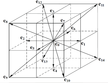
Figure 1: Schematic diagram of the D3Q15 model[31].

We consider the simulation of the incompressible Newtonian fluids where the LBM-D2Q9 and D3Q15 models [1] are adopted for the two- and three-dimensional calculations, respectively. In this section, the equation systems of the D3Q15 model are presented. For the two-dimensional ones, the readers are referred to our previous study [9]. The three-dimensional spatial distribution of the fluid velocities is shown in Figure 1 which can be expressed by

$$e_{\alpha}=\left\{\begin{array}[]{ll}(0,0,0)c&\alpha=0\\ (\pm 1,0,0)c,(0,\pm 1,0)c,(0,0,\pm 1)c&\alpha=1-6\\ (\pm 1,\pm 1,\pm 1)c&\alpha=7-14\end{array}\right.$$ (4)

where $c$ is termed by the lattice speed. The formulation of the lattice Bhatnagar-Gross-Krook model is

$$f_{\alpha}(r+e_{\alpha}\delta_{t},t+\delta_{t})=f_{\alpha}(r,t)-\frac{f_{\alpha}(r,t)-f_{\alpha}^{eq}(r,t)}{\tau_{f}}+F_{\alpha}\delta_{t}$$ (5)

$$g_{\alpha}(r+e_{\alpha}\delta_{t},t+\delta_{t})=g_{\alpha}(r,t)-\frac{g_{\alpha}(r,t)-g_{\alpha}^{eq}(r,t)}{\tau_{g}}+G_{\alpha}\delta_{t}$$ (6)

where $f_{\alpha}(r,t)$ and $g_{\alpha}(r,t)$ represent the fluid density and temperature distribution functions, respectively, $r=(x,y,z)$ stands for the space position vector, $t$ denotes time, and $\tau_{f}$ and $\tau_{g}$ denote the non-dimensional relaxation times which can be calculated by [17]

$$\tau_{f}=\dfrac{\sqrt{Pr}L_{c}u_{c}}{\sqrt{Ra}c_{s}^{2}\delta_{t}}+0.5$$ (7)

$$\tau_{g}=\dfrac{L_{c}u_{c}}{\sqrt{PrRa}c_{s}^{2}\delta_{t}}+0.5$$ (8)

where $c_{s}=c/\sqrt{3}$ is the lattice speed of sound, $L_{c}$ and $u_{c}=\sqrt{g\beta L_{c}\Delta T}$ are the characteristic length and velocity, respectively, and $Pr$ and $Ra$ are the Prandtl and Rayleigh numbers, respectively.

$$Pr=\frac{\nu_{f}}{\alpha_{f}}$$ (9)

$$Ra=\frac{g\beta\Delta TL_{c}^{3}}{\alpha_{f}\nu_{f}}$$ (10)

where $\nu_{f}$ is the kinematic viscosity of fluid, $\alpha_{f}$ is the thermal diffusivity, $g$ is the gravity, and $\beta$ is the thermal expansion coefficient. The source terms, $F_{\alpha}\delta_{t}$ and $G_{\alpha}\delta_{t}$, in Equations 5 and  6 are given in Section 2.2. The equilibrium density and temperature distribution functions, $f_{\alpha}^{eq}(r,t)$ and $g_{\alpha}^{eq}(r,t)$, can be written as

$$f_{\alpha}^{eq}(r,t)=\rho_{f}\omega_{\alpha}[1+3(e_{\alpha}\cdot u)+\frac{9}{2}(e_{\alpha}\cdot u)^{2}-\frac{3}{2}\mid u\mid^{2}]$$ (11)

$$g_{\alpha}^{eq}(r,t)=T\omega_{\alpha}[1+3(e_{\alpha}\cdot u)+\frac{9}{2}(e_{\alpha}\cdot u)^{2}-\frac{3}{2}\mid u\mid^{2}]$$ (12)

where the value of weights are: $\omega_{0}=2/9$, $\omega_{\alpha}=1/9$ for $\alpha=1-6$ and $\omega_{\alpha}=1/72$ for $\alpha=7-14$. $u$ denotes the macro velocity at each lattice node which can be calculated by $u=(\sum\limits_{\alpha=0}^{14}f_{\alpha}e_{\alpha}+\dfrac{1}{2}(\Delta T(\dfrac{u_{c}}{c})^{2}+F_{B})\delta_{t})/\rho_{f}$, the macro fluid density is $\rho_{f}=\sum\limits_{\alpha=0}^{14}f_{\alpha}$ and the macro temperature can be calculated by $T=\sum\limits_{\alpha=0}^{14}g_{\alpha}e_{\alpha}+\dfrac{1}{2}Q_{B}\delta_{t}$. The discrepancy of the formulations of $u$ and $T$ here with the conventional ones is due to the fact that they are modified by the momentum and heat flux [7]. For example, $F_{B}$ and $Q_{B}$ stand for the body force and heat source, respectively. $\Delta T(\dfrac{u_{c}}{c})^{2}$ represents the non-dimensional buoyancy caused by temperature gradients [21].

2.2 PIBM

Figure 2: Schematic diagram of the PIBM.

It is worthwhile mentioning that the PIBMs for the no-slip velocity and temperature boundary conditions share a fairly similar logical manner. The common idea is to obtain an accurate expression of the velocity or temperature difference between the two phases and then use it to make further modification on the behavior of the fluid flow field and solid particles. In this study, the heat conduction between the solid particles or particle and wall is not considered. For the sake of clarity, the two-dimensional schematic diagram of the PIBM is displayed with three-dimensional equation systems. As shown in Figure 2, the fluid is described using the Eulerian square lattices and the solid particles are denoted by the Lagrangian points moving in the flow field. The fluid density and temperature distribution functions on the solid particles are evaluated using the numerical extrapolation from the circumambient fluid points,

$$f_{\alpha}(X_{l},t)=L(X_{l},r)\cdot f_{\alpha}(r,t)$$ (13)

$$g_{\alpha}(X_{l},t)=L(X_{l},r)\cdot g_{\alpha}(r,t)$$ (14)

where $X_{l}(X,Y,Z)$ is the coordinates of the solid particles, the subscript ’$l$’ denotes the variable at the location of the Lagrangian particles. $L(X_{l},r)$ is the three-dimensional polynomials,

$$L(X_{l},r)=\sum\limits_{ijk}\left(\prod\limits_{l=1,l!=i}^{i_{max}}\frac{X-x_{ljk}}{x_{ijk}-x_{ljk}}\right)\left(\prod\limits_{m=1,m!=j}^{j_{max}}\frac{Y-y_{imk}}{y_{ijk}-y_{imk}}\right)\left(\prod\limits_{n=1,n!=k}^{k_{max}}\frac{Z-z_{ijn}}{z_{ijk}-z_{ijn}}\right)$$ (15)

where $i_{max}$, $j_{max}$ and $k_{max}$ are the maximum numbers of the Eulerian points used in the extrapolation as shown by blocks in Figure 2. With the movement of the solid particle, $f_{\alpha}(X_{l},t)$ will be further affected by the particle velocity, $U_{p}$,

$$f_{\beta}(X_{l},t+\delta_{t})=f_{\alpha}(X_{l},t)-2\omega_{\alpha}\rho_{f}\frac{e_{\alpha}U_{p}}{c_{s}^{2}}$$ (16)

and $g_{\alpha}(X_{l},t)$ will be further affected by the temperature difference between the solid particle and fluid, $\Delta T$ [21],

$$g_{\beta}(X_{l},t+\delta_{t})=g_{\alpha}(X_{l},t)-2\omega_{\alpha}\Delta T\dfrac{h}{\delta_{t}}$$ (17)

in Equations 16 and  17, the subscript $\beta$ represents the opposite direction of $\alpha$, and $h$ is the mesh spacing. Based on the momentum exchange between fluid and particles, the force density, $F_{f}(X_{l},t)$, at each solid particle can be calculated using $f_{\alpha}$ and $f_{\beta}$,

$$F_{f}(X_{l},t)=\sum\limits_{\beta}e_{\beta}[f_{\beta}(X_{l},t)-f_{\alpha}(X_{l},t)]$$ (18)

The effect on the flow fields from the solid boundary is the body force term $F_{\alpha}\delta_{t}$ in Equation 5, $F_{\alpha}$ can be expressed by

$$F_{\alpha}=\left(1-\frac{1}{2\tau_{f}}\right)\omega_{\alpha}\left(3\frac{e_{\alpha}-u}{c^{2}}+9\frac{e_{\alpha}\cdot u}{c^{4}}e_{\alpha}\right)F_{B}(r,t)$$ (19)

where

$$F_{B}(r,t)=\sum\limits_{l}F_{f}(X_{l},t)D_{ijk}(r_{ijk}-X_{l})A_{p}$$ (20)

The heat source $G_{\alpha}\delta_{t}$ in Equation 6 is one dimensional and can thus be directly given as

$$G_{\alpha}=\left(1-\frac{1}{2\tau_{g}}\right)\omega_{\alpha}Q_{B}$$ (21)

where

$$Q_{B}=\dfrac{u_{c}}{c\sqrt{PrRa}}(\sum\limits_{l}2\Delta T\dfrac{h}{\delta_{t}}D_{ijk}(r_{ijk}-X_{l})A_{p})$$ (22)

in Equations 20 and  22, $A_{p}$ is the cross-sectional area of the particle which is given as $A_{p}=0.25\pi d_{p}^{2}$, $d_{p}$ is the diameter of the particle. $D_{ijk}$ is used to restrict the feedback force to only take effect on the lattice nodes close to the solid particle and is given by

$$D_{ijk}(r_{ijk}-X_{l})=\frac{1}{h^{3}}\delta_{h}\left(\frac{x_{ijk}-X_{l}}{h}\right)\delta_{h}\left(\frac{y_{ijk}-Y_{l}}{h}\right)\delta_{h}\left(\frac{z_{ijk}-Z_{l}}{h}\right)$$ (23)

where

$$\delta_{h}(a)=\left\{\begin{array}[]{cc}\frac{1}{4}(1+cos(\frac{\pi a}{2})),&when\mid a\mid\leq 2\\ 0,&otherwise\\ \end{array}\right.$$ (24)

On the other hand, the fluid-solid interaction force exerted on the solid particle can be obtained as the reaction force of $F_{f}(X_{l},t)$,

$$F_{fpi}=-F_{f}(X_{l},t)A_{p}$$ (25)

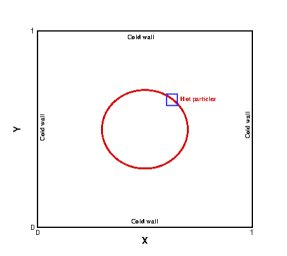
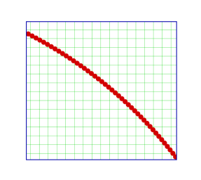
(a)                                               (b)

Figure 3: The schematic diagram of (a) square cavity with a concentric annulus and (b) local zoomed view.

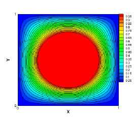
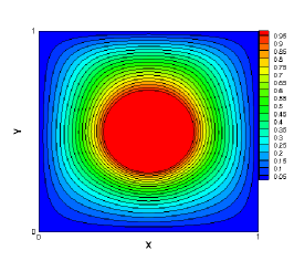
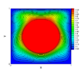
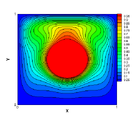
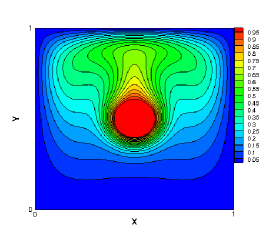
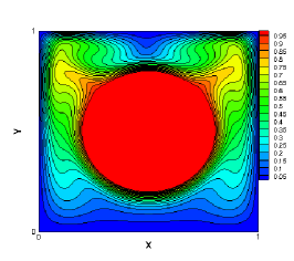
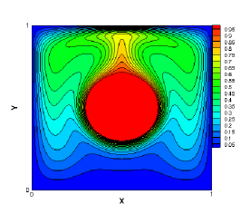
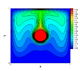
(a)                                 (b)                                 (c)

Figure 4: Isothermal contours of temperature distribution in the square cavity at different $Ra$ and $Ar$: (a)(top) $Ra=10^{4}$, $Ar=1.67$, (b)(top) $Ra=10^{4}$, $Ar=2.5$, (c)(top) $Ra=10^{4}$, $Ar=5$; (b)(middle) $Ra=10^{5}$, $Ar=1.67$, (b)(middle) $Ra=10^{5}$, $Ar=2.5$, (b)(middle) $Ra=10^{5}$, $Ar=5$; (c)(bottom) $Ra=10^{6}$, $Ar=1.67$, (c)(bottom) $Ra=10^{6}$, $Ar=2.5$, (c)(bottom) $Ra=10^{6}$, $Ar=5$.

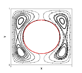
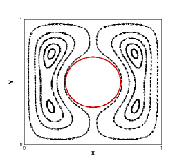
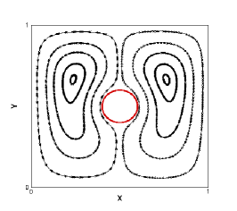
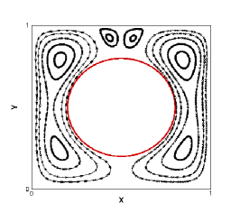
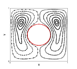
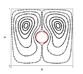
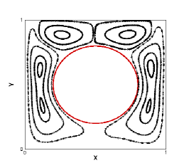
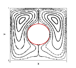
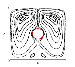
(a)                                 (b)                                 (c)

Figure 5: Isothermal contours of temperature distribution in the square cavity at different $Ra$ and $Ar$: (a)(top) $Ra=10^{4}$, $Ar=1.67$, (b)(top) $Ra=10^{4}$, $Ar=2.5$, (c)(top) $Ra=10^{4}$, $Ar=5$; (b)(middle) $Ra=10^{5}$, $Ar=1.67$, (b)(middle) $Ra=10^{5}$, $Ar=2.5$, (b)(middle) $Ra=10^{5}$, $Ar=5$; (c)(bottom) $Ra=10^{6}$, $Ar=1.67$, (c)(bottom) $Ra=10^{6}$, $Ar=2.5$, (c)(bottom) $Ra=10^{6}$, $Ar=5$.

2.3 Modeling of the particle-particle interactions

Since heat transfer between particle-particle and particle-wall is not considered, the remaining job is to monitor the trajectories of the solid particles and treat the inter-particle collisions properly. Based on the Newton’s second law of motion, the dynamic equations of the solid particle can be expressed as

$$m\frac{d^{2}r}{dt^{2}} = (1-\frac{\rho_{f}}{\rho_{p}})g+F_{fpi}$$ (26)

$$I\frac{d^{2}\theta}{dt^{2}} = \tau_{p}$$ (27)

where $m$ and $I$ are the mass and the moment of inertia of the particle, respectively. $r$ is the particle position and $\theta$ is the angular position. $\rho_{f}$ and $\rho_{p}$ are the densities of the fluid and particle, respectively. $\tau_{p}$ is the torque. Another considered force on the right hand side of Equation 26 is the fluid-particle interaction force $F_{fpi}$. When the particles collide directly with other particles or the walls, DEM is employed to calculate the collision force. In this study, the particles and walls are directly specified by material properties in the simulation such as density, Young’s modulus and friction coefficient. When the collisions take place, the theory of Hertz [32] is used for modeling the force-displacement relationship while the theory of Mindlin and Deresiewicz [33] is employed for the tangential force-displacement calculations. For particle of radius $R_{i}$ , Young’s modulus $E_{i}$ and Poisson’s ratios $\nu_{i}$, the normal force-displacement relationship between the colliding particles reads

$$F_{n}=\frac{4}{3}E^{*}R^{*1/2}\delta_{n}^{3/2}$$ (28)

where the equivalent Young’s modulus and radius can be calculated by $1/E^{*}=(1-\nu_{1}^{2})/E_{1}+(1-\nu_{2}^{2})/E_{2}$ and $1/R^{*}=1/R_{1}+1/R_{2}$, respectively.

The incremental tangential force arising from an incremental tangential displacement depends on the loading history as well as the normal force

$$\Delta T=8G^{*}r_{a}\theta_{k}\Delta\delta_{t}+(-1)^{k}\mu\Delta F_{n}(1-\theta_{k})$$ (29)

where $1/G^{*}=(1-\nu_{1}^{2})/G_{1}+(1-\nu_{2}^{2})/G_{2}$, $r_{a}=\sqrt{\delta_{n}R^{*}}$ is radius of the contact area. $\Delta\delta_{t}$ is the relative tangential incremental surface displacement, $\mu$ is the coefficient of friction, the value of $k$ and $\theta_{k}$ changes with the loading history.

3 Results and discussions

$Ra$	$Ar$	Present	Hu et al. [20]	Ren et al. [34]	Moukalled and Acharya [35]
	$5$	$2.041$	$2.038$	$2.051$	$2.071$
$10^{4}$	$2.5$	$3.179$	$3.184$	$3.161$	$3.331$
	$1.67$	$5.213$	$5.294$	$5.303$	$5.286$
	$5$	$3.760$	$3.778$	$3.704$	$3.825$
$10^{5}$	$2.5$	$4.989$	$4.917$	$4.836$	$5.080$
	$1.67$	$6.193$	$6.247$	$6.171$	$6.212$
	$5$	$6.025$	$6.095$	$5.944$	$6.107$
$10^{6}$	$2.5$	$8.831$	$8.934$	$8.546$	$9.374$
	$1.67$	$11.857$	$11.995$	$11.857$	$11.620$

Table 1: Comparison of computed average Nusselt numbers.

3.1 Natural convection in a two-dimensional square cavity with a concentric annulus

Natural convection in a two-dimensional square cavity has been a popular benchmark case for the verification of one’s numerical tools on heat transfer through fluid materials [35, 34, 20]. In this subsection, the case is employed to test the thermal LBM code coupling with the PIBM. An isothermal concentric annulus is planted in the center of the cavity as the heat source. The schematic diagram of the entire computational domain is shown in Figure 3(a). It should be stressed that the concentric annulus here is constructed by small isothermal particles with uniform size as shown in Figure 3(b). The positions of the solid particles are artificially set stagnant to prevent them following down under the action of gravity. The length and height of the cavity are $1$, respectively. We consider three sizes of concentric annulus. The ratios of the cavity length to the annulus diameter $Ar$ are $1.67$, $2.5$ and $5$. We use $250\times 250$ meshes to cover the whole computational domain. The diameter of the solid particles is $h/2$. $Ra$ of interest is ranging from $10^{4}$ to $10^{6}$ and $Pr=0.71$. The non-dimensional temperature is set $1$ and $0$ at the concentric annulus and the surrounding cold walls, respectively. The initial temperature of the stagnant fluid is $0.5$. The remainder parameters relevant to the simulations are $L_{c}=1$ and $u_{c}=0.25$.

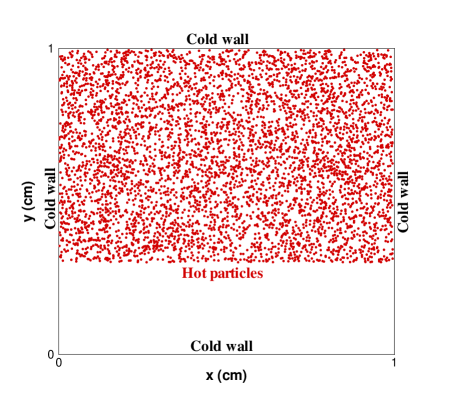
Figure 6: Schematic diagram of the PIBM.

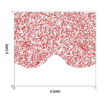
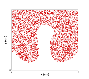
(a)                                               (b)
  
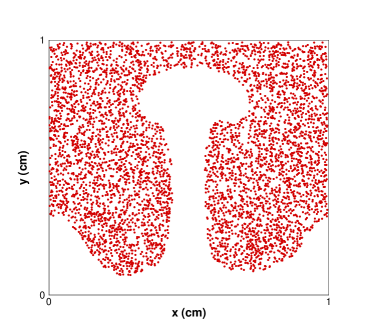
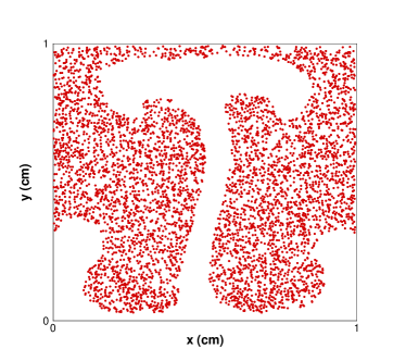
(c)                                               (d)

Figure 7: Positions of the $5000$ particles without heat transfer at time (a) $t=2.5s$, (b) $t=5.0s$, (c) $t=7.5s$, (d) $t=10.0s$.

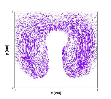
(a)                                               (b)
  
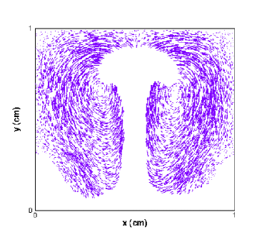
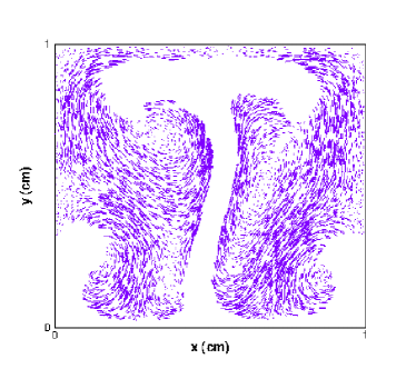
(c)                                               (d)

Figure 8: Velocity distribution of the $5000$ particles without heat transfer at time (a) $t=2.5s$, (b) $t=5.0s$, (c) $t=7.5s$, (d) $t=10.0s$.

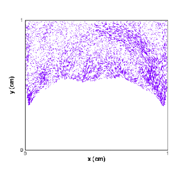
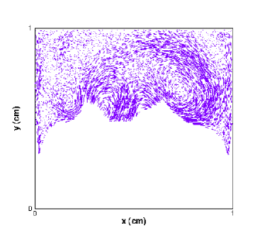
(a)                                               (b)
  
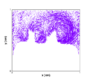
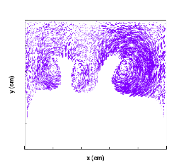
(c)                                               (d)

Figure 9: Velocity distribution of the $5000$ particles with heat transfer at time (a) $t=2.5s$, (b) $t=5.0s$, (c) $t=7.5s$, (d) $t=10.0s$.

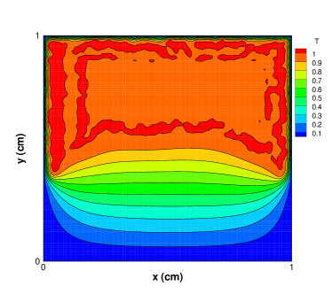
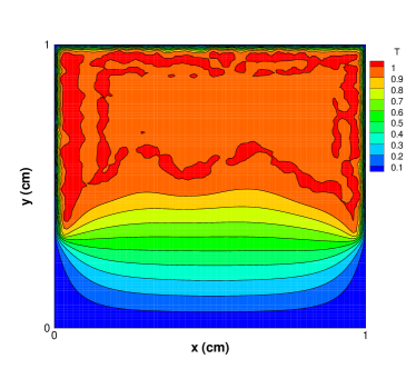
(a)                                               (b)
  
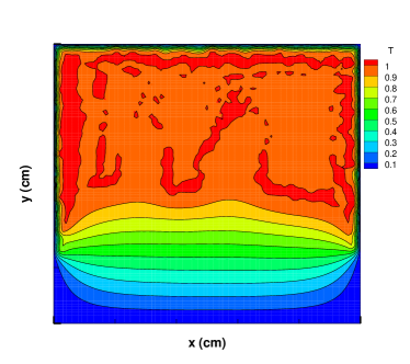
(c)                                               (d)

Figure 10: Temperature distribution in the cavity at time (a) $t=2.5s$, (b) $t=5.0s$, (c) $t=7.5s$, (d) $t=10.0s$.

The isothermal contours of temperature distribution in the cavity at different $Ra$ and $Ar$ are displayed in Figure 4. As shown, the temperature distribution is affected by both $Ra$ and $Ar$. The strength of convection is stronger as $Ra$ increases which gives rise to much more complex isothermal patterns. The thermal boundary at the lower surface of concentric annulus is thinner at the higher $Ra$ for each $Ar$. As for the region just above the concentric annulus, a gradual changing of temperature can be observed at $Ra=10^{4}$ which means that heat conduction mainly dominates at this region at low $Ra$. However, when $Ra$ increases, a crown-like region with high temperature is formed due to the high effect of convection. Namely, the temperature distribution is more affected by the fluid velocity field at higher $Ra$. The streamlines in the cavity at different $Ra$ and $Ar$ are displayed in Figure 5. Similar to the temperature fields, the streamlines are symmetrically distributed about the perpendicular bisector of the concentric annulus. The influence of $Ra$ on the flow field is obvious. As $Ra$ increases, two more counter-rotating vortexes are shown between the upper surface of the concentric annulus and the top wall of the cavity when $Ar=1.67$, the two vortexes besides the concentric annulus merge into a big one, respectively, when $Ar=2.5$ and two more counter-rotating vortexes can be observed below the the concentric annulus when $Ar=5$. All these observations have very good agreements with the previous numerical results under the same conditions [34, 20]. Quantitative comparison of computed average Nusselt numbers is shown in Table 1. In this study, we calculate the average Nusselt number following Hu et al. [20]:

$$\overline{Nu}=\dfrac{\sum\limits_{l}\Delta ThA_{p}}{\delta_{t}k(T_{hot}-T_{\infty})}$$ (30)

where $k$ is the thermal conductivity. As can be seen from Table 1, the LBM-PIBM scheme also does a good job of predicting reasonable $\overline{Nu}$ and thus is a promising method for simulating the free convection problems.

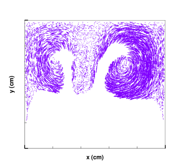
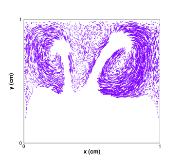
(a)                                               (b)
  
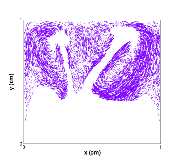
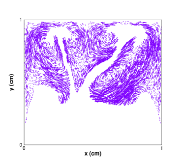
(c)                                               (d)

Figure 11: Velocity distribution of the $5000$ particles with heat transfer at time (a) $t=12.5s$, (b) $t=15.0s$, (c) $t=17.5s$, (d) $t=20.0s$.

3.2 Sedimentation of two-dimensional isothermal particles in fluid

From this subsection, fully coupled LBM-PIBM-DEM simulations are performed. The main target of this and next subsections are to investigate the temperature distribution feature in the cavity during particle sedimentation and the effect of the thermal buoyancy on particle behaviors. The current numerical results are compared with the ready-made cases in our previous study without considering heat transfer [13].

In the two-dimensional simulation, we consider a $1$ $cm$ $\times$ $1$ $cm$ cavity with $5000$ two-dimensional particles. The calculating mesh for the LBM is $100\times 100$. The diameter of the particles is $0.25\times 10^{-2}$ $cm$ or $h/d_{p}=4$. The initially spacial condition is exactly the same as the two-dimensional case in [13]. Firstly, the $5000$ particles are randomly generated in the upper three-fifths domain and then deposit under the effect of the gravitational force, $g=9.8$ $m\cdot s^{-2}$. The density ratio between solid and fluid is $1.01$, $Ra=10^{4}$, $Pr=0.71$, $L_{c}=1$ and $u_{c}=0.25$. The non-dimensional temperature is set $1$ and $0$ at the solid particles and the four surrounding cold walls, respectively. The initial temperature of the stagnant fluid is $0.5$. At last, the parameters responsible for the collision between the solid particles are $E=68.95$ $GPa$ and $\nu=0.33$. For the sake of investigating the effect of the thermal buoyancy on particle behavior, two parallel simulations are carried out with and without considering heat transfer. In other words, the heat-introduced buoyancy would be ignored in the case without considering heat transfer.

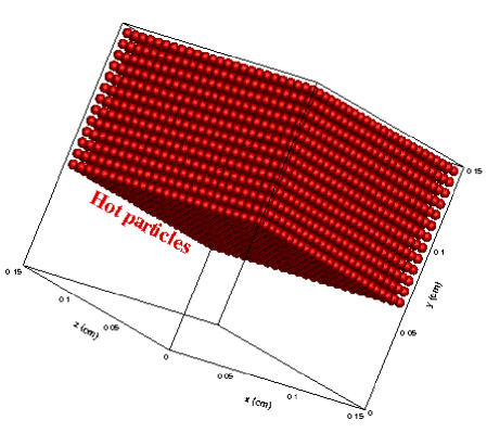
Figure 12: Positions of the 8125 isothermal particles at time $t=0.0s$.

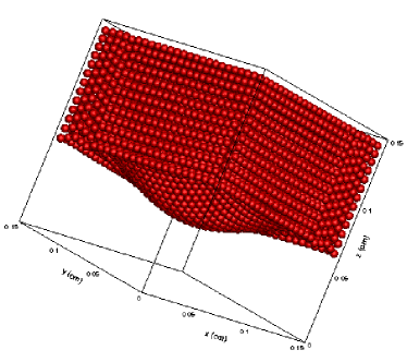
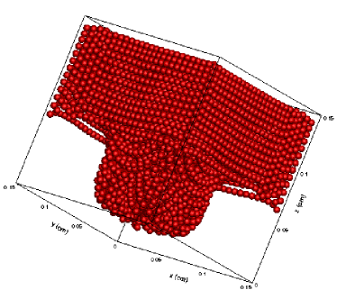
(a)                                               (b)
  
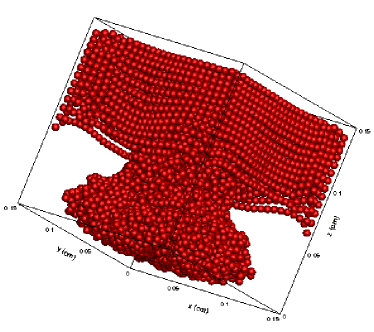
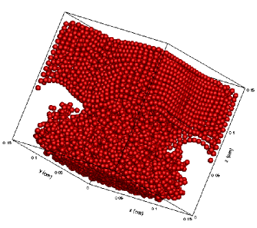
(c)                                               (d)

Figure 13: Positions of the $8125$ isothermal particles without heat transfer at time (a) $t=2.5s$, (b) $t=5.0s$, (c) $t=7.5s$, (d) $t=10.0s$.

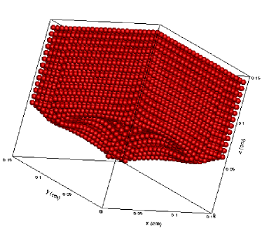
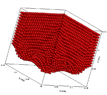
(a)                                               (b)
  
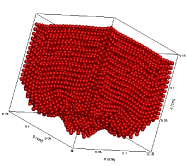
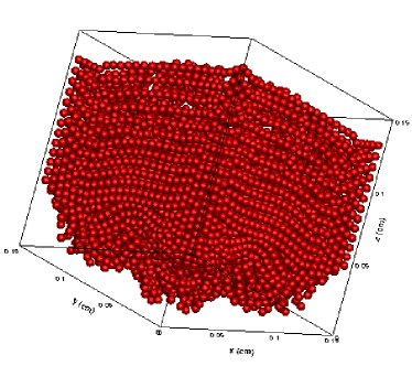
(c)                                               (d)

Figure 14: Positions of the $8125$ isothermal particles with heat transfer at time (a) $t=2.5s$, (b) $t=5.0s$, (c) $t=7.5s$, (d) $t=10.0s$.

Figure 7 displays the particle distribution during the beginning $10.0s$ when heat transfer is not considered. As shown, the flow fluid at lower position is swallowed into the particle aggregate forming a fluid pocket with a mushroom shape. This typical two-dimensional phenomenon is regarded as the so-called Rayleigh-Taylor instability which has been well investigated by several studies [36, 5, 9, 13]. The solid particles prefer to settle around the fluid column until being shot up by the upthrust flow field. This process can be clearly seen from the distribution map of particle velocities as shown in Figure 8. Firstly, two vortexes with solid particles are formed in the interior of the cavity. Then, the height of these two vortexes rises meanwhile the downthrust of the particle streams introduces two more small vortexes close to the lower corners of the cavity due to the intimate interaction between the particle and fluid as shown in Figure 8(d).

However, the sedimentation is fairly delayed when heat transfer is considered. Figure 9 shows the velocity distribution of the $5000$ particles with heat transfer at the same moments as Figure 8. Comparing with the case without heat transfer, the settling velocities of the thermal particles are significantly lower. This is due to the fact that the particle temperature is higher than the surrounding fluid. The fluid receives heat from the solid particles meanwhile the wall temperature is the lowest. Therefore, the fluid temperature increases at the location close to the solid particles whereas decreases close to the cold walls as shown in Figure 10. It can be seen that the high temperature region is in conformity with the particle position. The temperature gradients make the density differences in the fluid occur. This gives rise to that the fluid in the cavity interior becomes less dense and rises. The solid particles at this region also rise with the ascending fluid which prevents the evolution in Figure 7. Besides the overall settling velocity, there is also large discrepancy on the particle distribution patterns when heat transfer is considered. Instead of one fluid pocket with a mushroom shape in Figure 7, two branches are generated at the interface of solid and fluid as shown in Figure 9. The whole system is more unstable when heat transfer is introduced.

Figure 11 displays the further evolution of the velocity distribution of the $5000$ particles when heat transfer is considered. As shown, the above-mentioned two branches in Figure 9 grow to two fluid pockets also with mushroom shapes. The two heads do not rise vertically any longer but towards the upper corners of the cavity. This phenomenon is not observed in the simulation without heat transfer before  [36, 5, 9, 13]. It seems that the thermal buoyancy totally breaks the original rule and introduces more intensive fluid-particle interactions.

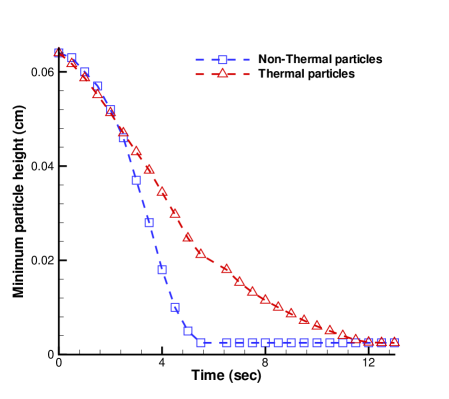
Figure 15: Minimum particle height versus time with and without heat transfer.

3.3 Sedimentation of three-dimensional isothermal particles in fluid

For the sake of conducting further investigation on the effect of thermal buoyancy on the particle behaviors, in this subsection, a three-dimensional $0.15$ $cm$ $\times$ $0.15$ $cm$ $\times$ $0.15$ $cm$ cubic cavity is considered with six cold walls. The calculating mesh for the LBM is $15\times 15\times 15$. The diameter of the solid particles is $0.5\times 10^{-2}$ $cm$ or $h/d_{p}=2$. The initial spacial set of the three-dimensional case is the same as the three-dimensional case in  [13] which also can be seen in Figure 12. $8125$ particles are regularly planted in the upper three-fifths domain of the cubic cavity with an identical separation distance, $0.001$ $cm$. This leads to the local porosity, $0.719$. The non-dimensional temperature is set $1$ and $0$ at the solid particles and the six surrounding cold walls, respectively. The initial temperature of the stagnant fluid is $0.5$. Other physical parameters of the fluid and particles are the same as the two-dimensional case in Section 3.2. Similarly, two parallel simulations are carried out with and without considering heat transfer.

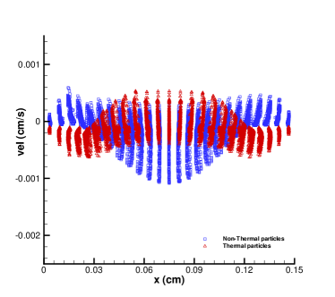
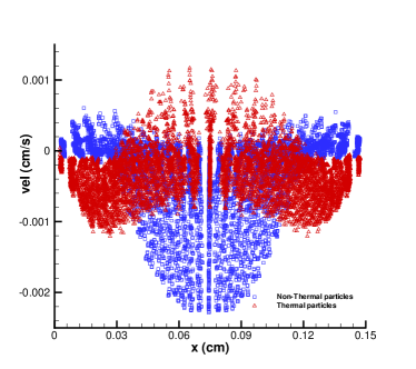
(a)                                               (b)
  
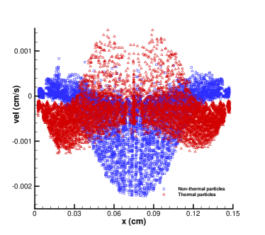
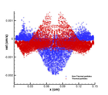
(c)                                               (d)

Figure 16: Particle deposition velocity along the x-direction with and without heat transfer at time (a) $t=2.5s$, (b) $t=5.0s$, (c) $t=7.5s$, (d) $t=10.0s$.

Figure 13 displays the three-dimensional particle distribution during the beginning $10.0s$ when heat transfer is not considered. As shown, unlike the two-dimensional case, the three-dimensional particles in the center region settle more efficiently than others. The particles close to the walls move fairly slow as a result of the no-slip boundary condition employed between the fluid and wall. The particle matrix is rapidly hollowed out forming a downstream particle-constructed pestle. The particle-constructed pestle falls down directly until impacts on the bottom and then the particles scatter in all directions. This process has been reported in [13, 37] without considering heat transfer.

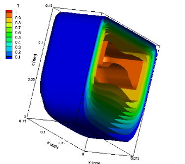
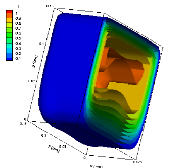
(a)                                               (b)
  
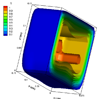
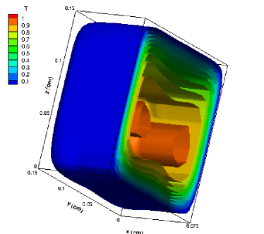
(c)                                               (d)

Figure 17: Isothermal surfaces in the cubic cavity at time (a) $t=2.5s$, (b) $t=5.0s$, (c) $t=7.5s$, (d) $t=10.0s$.

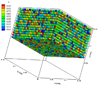
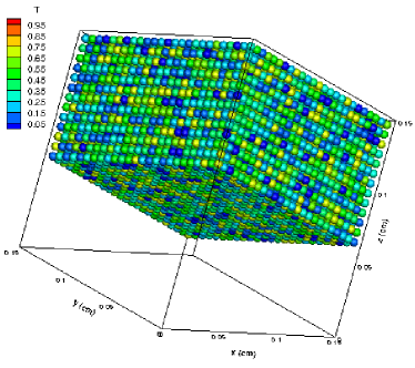
(a)                                               (b)
  
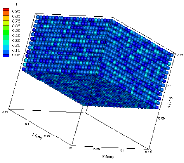
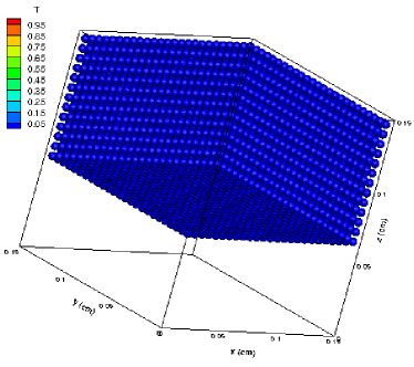
(c)                                               (d)

Figure 18: The $8125$ thermosensitive particles colored by temperature at time (a) $t=0.0s$, (b) $t=0.01s$, (c) $t=0.03s$, (d) $t=0.12s$.

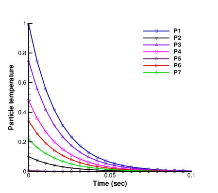
Figure 19: Temperature evolution histories of $7$ particles.

Figure 14 shows the particle distribution of the $8125$ particles with heat transfer at the same moments as Figure 13. It can be seen that the particle behaviors are obviously different to the former case when heat transfer is not considered. Instead of forming a particle-constructed pestle in the center region, the bottom surface of the isothermal particle aggregate is more fluctuant with bulges. This finding is in line with the two-dimensional one, the interface of the solid and lower fluid is more complex when heat transfer is considered. At $t=2.5s$, the particle distributions exhibit completely contrary trends with and without heat transfer. It shows a hump in Figure 13(a) whereas a hollow in Figure 14(a). The discrepancy is due to the high thermal buoyancy in the interior, the particles in the corners have the priority to settle since the temperature in these regions is low. The subsequent sedimentation feature in Figure 14 follows this trend where the bulging at the four corner region can be observed.

Figure 15 shows the changing history of the minimum particle height in the two cases. This is a good measurement of the overall sedimentation efficiency. It can be seen that the two profiles are quite comparable before $2.4s$. Then, the non-thermal particles begin to accelerate whereas the sedimentation of the thermal particles is significantly delayed by the buoyancy. Detailed comparison between the particle deposition velocity along the x-direction with and without heat transfer is given in Figure 16. The contrary distribution of the particle deposition velocity validates the afore-mentioned observations.

At last, the temperature distributions in the cubic cavity are displayed in Figure 17 in terms of isothermal surfaces. The cavity is dissected at the bisector of the x-direction which visualizes the temperature distribution feature inside. It is shown that the temperature at the interior of the particle aggregate is the highest. The thermal buoyancy at this region is also the highest and thus the solid particles possess the highest upwards velocities as shown in Figure 16. The location of the heat core moves downwards with sedimentation of the solid particles. The temperature between the particle aggregate and surrounding walls changes gradually due to the low $Ra$ adopted.

3.4 Sedimentation of three-dimensional thermosensitive particles in fluid

In this subsection, three-dimensional thermosensitive particles are considered in the same model as Section 3.3. Different to all the above cases where the temperature of the solid particles is constant. Here, the thermosensitive particles could lose or receive heat according to the surrounding temperature. The initial temperature of the $8125$ thermosensitive particles is set randomly between $0$ and $1$ as shown in Figure 18 (a). The walls are set cold with $0$ temperature. The initial temperature of the stagnant fluid is $0.5$. All the other computational parameters are the same as Section 3.3.

Since the walls are cold, it can be expected that the temperature of the whole system would reach a final steady-state which is the same as the wall temperature. This process can be clearly observed in Figure 18 which displays the particle temperature distribution at different time instants. Along with that the cold walls keep sucking heat, the temperature of the whole system drops rapidly to the steady-state value. Here, we monitor the temperature evolution histories of $7$ solid particles randomly picked from the assembly. As shown in Figure 19, the different profiles again indicate the feature of the cooling process.

4 Concluding remarks

In this paper, the LBM-PIBM-DEM scheme was employed to solve thermal interaction problems between spherical particles and fluid. The LBM was adopted to solve the fluid flow and temperature fields, the PIBM was responsible for the no-slip velocity and temperature boundary conditions at the particle surface, and the kinematics and trajectory of the particles were evaluated by the DEM.

Four case studies were implemented to certify the capability of the proposed coupling scheme. First, numerical simulation of natural convection in a two-dimensional square cavity with an isothermal concentric annulus was carried out for verification purpose. Then, sedimentation of two- and three-dimensional isothermal particles in fluid was numerically studied. The instantaneous temperature distribution in the cavity was captured. The effect of thermal buoyancy on the particle behaviors was discussed. Finally, sedimentation of three-dimensional thermosensitive particles in fluid was numerically investigated. Our results revealed that the thermal buoyancy has a great effect on the particle behaviors both in two- and three-dimensional simulations. When heat transfer is considered, the interface between the solid particle aggregate and lower fluid is more unstable. The heat buoyancy could influence on the sedimentation efficiency of the solid particles very much. All the simulations demonstrate that the LBM-PIBM-DEM coupling scheme is a promising one for the solution of complex fluid-particle interaction problems with heat transfer.

One critical assumption made in this study is that the heat conduction between solid particles or particle and wall is ignored. This assumption is reasonable when intense inter-particle collisions dominate the system, for example, the fore part of the sedimentation process where the collision process is instant. Nevertheless, this may be against those actual engineering processes where the heat conduction between solids cannot be neglected [26, 28]. As shown in Section 3.1, the LBM-PIBM scheme is competent to pure natural convection problems. Further meshing on the solid particle can be performed to calculate heat conduction through particles like Feng et al. [22, 23]. This work is interesting but will of course increase the calculation burden. An alternative approach is to consider fluid flow and heat transfer just at the particle scale as done in [26, 27, 28, 29]. Therefore, it is in the authors’ opinion that the current LBM-PIBM-DEM scheme is more suitable for dynamic processes such as gas fluidization, hydrocyclone and pneumatic conveying. It can also be used to generate sub-particle information to support particle scale modeling.

References

References

- [1] Qian, YH and d’Humières, Dominique and Lallemand, Pierre, Lattice BGK models for Navier-Stokes equation, EPL (Europhysics Letters) 17 (6) (1992) 479.
- [2] P. Cundall, A computer model for simulating progressive large scale movements in blocky system, In: Muller led, ed. Proc Symp Int Soc Rock Mechanics, Rotterdam: Balkama A A 1 (1971) 8–12.
- [3] H. H. Hu, Direct simulation of flows of solid-liquid mixtures, International Journal of Multiphase Flow 22 (2) (1996) 335–352.
- [4] C. S. Peskin, Numerical analysis of blood flow in the heart, Journal of Computational Physics 25 (3) (1977) 220 – 252.
- [5] Z.-G. Feng, E. E. Michaelides, The immersed boundary-lattice Boltzmann method for solving fluid-particles interaction problems, Journal of Computational Physics 195 (2) (2004) 602 – 628.
- [6] Z.-G. Feng, E. E. Michaelides, Proteus: a direct forcing method in the simulations of particulate flows, Journal of Computational Physics 202 (1) (2005) 20 – 51.
- [7] X. Niu, C. Shu, Y. Chew, Y. Peng, A momentum exchange-based immersed boundary-lattice Boltzmann method for simulating incompressible viscous flows, Physics Letters A 354 (3) (2006) 173 – 182.
- [8] J. Wu, C. Shu, Particulate Flow Simulation via a Boundary Condition-Enforced Immersed Boundary-Lattice Boltzmann Scheme, Communications in Computational Physics 7 (2010) 793–812.
- [9] H. Zhang, Y. Tan, S. Shu, X. Niu, F. X. Trias, D. Yang, H. Li, Y. Sheng, Numerical investigation on the role of discrete element method in combined LBM-IBM-DEM modeling, Computers & Fluids 94 (2014) 37 – 48.
- [10] A. B. Yu, B. H. Xu, Particle-scale modelling of gas–solid flow in fluidisation, Journal of Chemical Technology and Biotechnology 78 (2-3) (2003) 111–121.
- [11] Y. Tan, H. Zhang, D. Yang, S. Jiang, J. Song, Y. Sheng, Numerical simulation of concrete pumping process and investigation of wear mechanism of the piping wall, Tribology International 46 (1) (2012) 137 – 144.
- [12] H. Zhang, Y. Tan, D. Yang, F. X. Trias, S. Jiang, Y. Sheng, A. Oliva, Numerical investigation of the location of maximum erosive wear damage in elbow: Effect of slurry velocity, bend orientation and angle of elbow, Powder Technology 217 (2012) 467 – 476.
- [13] H. Zhang, F. X. Trias, A. Oliva, D. Yang, Y. Tan, Y. Sheng, Effect of collisions on the particle behavior in a turbulent square duct flow, Powder Technology 269 (2015) 320–336.
- [14] H. Zhang, F. X. Trias, A. Oliva, D. Yang, Y. Tan, S. Shu, Y. Sheng, PIBM: Particulate immersed boundary method for fluid–particle interaction problems , Powder Technology 272 (2015) 1 – 13.
- [15] K. Han, Y. Feng, D. Owen, Coupled lattice Boltzmann and discrete element modelling of fluid–particle interaction problems, Computers and Structures 85 (11-14) (2007) 1080 – 1088.
- [16] X. Cui, J. Li, A. Chan, D. Chapman, Coupled DEM-LBM simulation of internal fluidisation induced by a leaking pipe, Powder Technology 254 (2014) 299–306.
- [17] X. He, S. Chen, G. D. Doolen, A novel thermal model for the lattice boltzmann method in incompressible limit, Journal of Computational Physics 146 (1) (1998) 282–300.
- [18] C. Shu, X. Niu, Y. Chew, A lattice Boltzmann kinetic model for microflow and heat transfer, Journal of statistical physics 121 (1-2) (2005) 239–255.
- [19] K. Han, Y. Feng, D. Owen, Modelling of thermal contact resistance within the framework of the thermal lattice boltzmann method, International Journal of Thermal Sciences 47 (10) (2008) 1276–1283.
- [20] Y. Hu, X.-D. Niu, S. Shu, H. Yuan, M. Li, Natural Convection in a Concentric Annulus: A Lattice Boltzmann Method Study with Boundary Condition-Enforced Immersed Boundary Method, Advances in Applied Mathematics and Mechanics 5 (2013) 321–336.
- [21] Y. Hu, D. Li, S. Shu, X. Niu, Study of multiple steady solutions for the 2d natural convection in a concentric horizontal annulus with a constant heat flux wall using immersed boundary-lattice boltzmann method, International Journal of Heat and Mass Transfer 81 (2015) 591–601.
- [22] Y. Feng, K. Han, C. Li, D. Owen, Discrete thermal element modelling of heat conduction in particle systems: Basic formulations, Journal of Computational Physics 227 (10) (2008) 5072–5089.
- [23] Y. Feng, K. Han, D. Owen, Discrete thermal element modelling of heat conduction in particle systems: Pipe-network model and transient analysis, Powder Technology 193 (3) (2009) 248–256.
- [24] H. Gan, J. Chang, J. J. Feng, H. H. Hu, Direct numerical simulation of the sedimentation of solid particles with thermal convection, Journal of Fluid Mechanics 481 (2003) 385–411.
- [25] Z.-G. Feng, E. E. Michaelides, Heat transfer in particulate flows with direct numerical simulation (DNS), International Journal of Heat and Mass Transfer 52 (3) (2009) 777–786.
- [26] Z. Y. Zhou, A. B. Yu, P. Zulli, Particle scale study of heat transfer in packed and bubbling fluidized beds, AIChE Journal 55 (4) (2009) 868–884.
- [27] Z. Y. Zhou, A. B. Yu, P. Zulli, A new computational method for studying heat transfer in fluid bed reactors, Powder Technology 197 (1) (2010) 102–110.
- [28] Q. F. Hou, Z. Y. Zhou, A. B. Yu, Computational study of the effects of material properties on heat transfer in gas fluidization, Industrial & Engineering Chemistry Research 51 (35) (2012) 11572–11586.
- [29] Q. F. Hou, Z. Y. Zhou, A. B. Yu, Computational study of heat transfer in a bubbling fluidized bed with a horizontal tube, AIChE Journal 58 (5) (2012) 1422–1434.
- [30] Z.-G. Feng, S. G. Musong, Direct numerical simulation of heat and mass transfer of spheres in a fluidized bed , Powder Technology 262 (2014) 62 – 70.
- [31] J. Wu, C. Shu, An improved immersed boundary-lattice Boltzmann method for simulating three-dimensional incompressible flows, Journal of Computational Physics 229 (13) (2010) 5022 – 5042.
- [32] K. Johnson, Contact mechanics, Cambridge University Press, Cambridge.
- [33] R. Mindlin, H. Deresiewicz, Elastic spheres in contact under varying oblique forces, Journal of Applied Mechanics 20 (1953) 327–344.
- [34] W. Ren, C. Shu, J. Wu, W. Yang, Boundary condition-enforced immersed boundary method for thermal flow problems with dirichlet temperature condition and its applications, Computers & Fluids 57 (2012) 40–51.
- [35] F. Moukalled, S. Acharya, Natural convection in the annulus between concentric horizontal circular and square cylinders, Journal of Thermophysics and Heat Transfer 10 (3) (1996) 524–531.
- [36] R. Glowinski, T.-W. Pan, T. I. Hesla, D. D. Joseph, A distributed lagrange multiplier/fictitious domain method for particulate flows, International Journal of Multiphase Flow 25 (5) (1999) 755–794.
- [37] M. Robinson, M. Ramaioli, S. Luding, Fluid-particle flow simulations using two-way-coupled mesoscale SPH-DEM and validation, International Journal of Multiphase Flow 59 (2014) 121 – 134.