Heat asymmetries in nanoscale conductors: The role of decoherence and inelasticity

Abstract

We investigate the heat flow between different terminals in an interacting coherent conductor when inelastic scattering is present. We illustrate our theory with a two-terminal quantum dot setup. Two types of heat asymmetries are investigated: electric asymmetry $\Delta_{E}$, which describes deviations of the heat current in a given contact when voltages are exchanged, and contact asymmetry $\Delta_{C}$, which quantifies the difference between the power measured in two distinct electrodes. In the linear regime, both asymmetries agree and are proportional to the Seebeck coefficient, the latter following at low temperature a Mott-type formula with a dot transmission renormalized by inelasticity. Interestingly, in the nonlinear regime of transport we find $\Delta_{E}\neq\Delta_{C}$ and this asymmetry departure depends on the applied bias configuration. Our results may be important for the recent experiments by Lee et al. [Nature (London) 498, 209 (2013)], where these asymmetries were measured.

I Introduction

Thermoelectrical transport at the nanoscale is a phenomenon of wide interest due to its fundamental and applied perspectives Sánchez and Linke (2014). From the practical point of view, nanostructures spur a wide range of promising thermoelectric applications such as thermocouples Kim et al. (2012), local refrigerators Shakouri (2006), thermal transistors Giazotto et al. (2006), and thermal rectifiers Terraneo et al. (2002), among others. The conversion of waste heat into electricity seems to be more efficient at the nanoscale than at macroscopic scales Heremans et al. (2013). The fast pursuit toward higher efficiency values of the generated electrical power in relation to the supplied heat has reached remarkable results Snyder and Toberer (2008); Li et al. (2010). However, related fundamental issues such as the electronic heat flow traversing a nanodevice still remain poorly understood mainly because thermal current is not easily accessible in an experiment Jezouin et al. (2013). In many aspects, heat flow inherently differs from its electrical counterpart and can reveal information about the number of channels available for transport Molenkamp et al. (1992), the presence of interactions Kane et al. (1997), properties of single-particle wave functions Battista et al. (2013), or even superconducting phase differences Spilla et al. (2014).

Recent works have investigated both experimentally and theoretically the heat current in atomic-scale junctions Lee et al. (2013); Zotti et al. (2014). Importantly, power dissipation at atomic scales depends strongly on the way in which the transmission probability varies with energy. Thus, for nanostructures showing a strongly energy-dependent transmission, the measured heat flux is shared quite asymmetrically among the contacts whereas for those systems with a weakly energy-dependent transmission the heat asymmetry is strongly suppressed Lee et al. (2013). This conclusion assumes that energy exchange between carriers occurs elastically. However, in molecular or atomic junctions, inelastic processes can be of critical importance when internal degrees of freedom such as rotational or vibrational modes come into play Paulsson and Datta (2003); Frederiksen et al. (2004); Koch et al. (2004); Galperin et al. (2007); Finch et al. (2009); Entin-Wohlman and Aharony (2012); Zimbovskaya (2014). As a consequence, these can alter the physical scenario. The fundamental question addressed in this work is precisely how the heat current asymmetry is affected by inelastic processes. We are interested in the contact asymmetry $\Delta_{C}$, which measures differences between the source ($\mathcal{J}_{1}$) and the drain ($\mathcal{J}_{2}$) heat currents, and the electric asymmetry $\Delta_{E}$, which quantifies the heat-current asymmetry in a given electrode when the applied voltages $V_{1}$ and $V_{2}$ are exchanged:

$$\Delta_{C} =\mathcal{J}_{1}(V_{1},V_{2})-\mathcal{J}_{2}(V_{1},V_{2})\,,$$ (1)

$$\Delta_{E} =\mathcal{J}_{1}(V_{1},V_{2})-\mathcal{J}_{1}(V_{2},V_{1})\,.$$ (2)

Furthermore, even when only elastic processes are present, dephasing mechanisms can also take place. Therefore, it is also natural to ask how heat is partitioned among the different electronic reservoirs in the presence of dephasing.

To examine both issues, we use the voltage Büttiker (1988); D’Amato and Pastawski (1990) and dephasing de Jong and Beenakker (1996); van Langen and Büttiker (1997) probe models, recently generalized to treat heat-current flows Saito et al. (2011); Sánchez and Serra (2011); Caso et al. (2012); Bedkihal et al. (2013); Bergfield et al. (2013); Apertet et al. (2013); Brandner and Seifert (2013); Meair et al. (2014). In these formulations, inelastic and dephasing processes are incorporated by considering a fictitious terminal attached to the quantum system in such a way that the net electrical and heat currents flowing through the probe vanish. In particular, for a voltage probe a carrier that enters the probe with a given energy is reemitted into the conductor with an unrelated energy. In contrast, when only dephasing processes are present, the energy-resolved heat and charge currents are identically zero at each energy. Since the model is independent of the microscopic details of the actual scattering mechanisms, the results are simple to understand and can be applied to a large variety of systems.

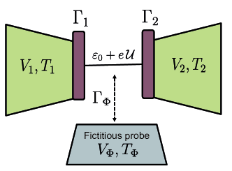
Figure 1: Schematic of a generic nanoconductor with energy level $\varepsilon_{0}$ in the presence of a voltage $V_{\Phi}$ and temperature $T_{\Phi}$ probes and coupled to left and right reservoirs by tunnel couplings $\Gamma_{1}$ and $\Gamma_{2}$. Here, $\Gamma_{\Phi}$ is the tunnel coupling with the probe. $V_{\Phi}$ and $T_{\Phi}$ adjust themselves in order to cancel the net flow of heat and charge through the probe. The internal potential in the conductor is denoted with ${\cal U}$.

Our theory is illustrated with a prototypical model for mesoscopic systems: a localized state (representing many different quantum systems, i.e., atomic or molecular junctions, quantum dots, etc.) attached to two electronic reservoirs and subject to different chemical and temperature biases, as depicted in Fig. 1.

II Theoretical model

When a mesoscopic conductor is coupled to $i=1\cdots N$ electronic reservoirs and is driven out of equilibrium by electrostatic fields $\{V_{i}\}$ or temperature gradients $\{\theta_{i}\}$, a flow of charge and energy from the reservoirs toward the conductor is established. Charge conservation dictates that all stationary charge flows add up to zero, $\sum_{i=1\cdots N}\mathcal{I}_{i}=0$, whereas the sum of thermal currents must include the Joule heating term, $\sum_{i=1\cdots N}(\mathcal{J}_{i}+\mathcal{I}_{i}V_{i})=0$. Within the scattering approach formalism, the flows read as Butcher (1990)

$$\mathcal{I}_{i}=\frac{2e}{h}\sum_{j}\int dEA_{ij}f_{j}(E)\,,$$ (3)

$$\mathcal{J}_{i}=\frac{2}{h}\sum_{j}\int dE\left(E-\mu_{i}\right)A_{ij}f_{j}(E)\,.$$ (4)

The factor $2$ originates from spin degeneracy since we do not consider external magnetic fields. The heat current $\mathcal{J}_{i}=\mathcal{J}_{i}^{E}-V_{i}\mathcal{I}_{i}$ is given by sum of the energy current $\mathcal{J}_{j}^{E}=(2/h)\sum_{j}\int dE(E-E_{F})A_{ij}f_{j}(E)$ and the associated Joule dissipating heat power $V_{j}\mathcal{I}_{j}$. The electrochemical potential in reservoir $i$ is defined as $\mu_{i}=E_{F}+eV_{i}$ with $E_{F}$ the Fermi energy, and $f_{j}(E)=\left[1+\exp{\left((E-\mu_{j})/k_{B}T_{j}\right)}\right]^{-1}$ is the Fermi-Dirac distribution function. Each terminal has temperature $T_{i}=\theta+\theta_{i}$, obtained from a temperature shift $\theta_{i}$ with respect to the background temperature $\theta$. The elements $A_{ij}=\operatorname{Tr}[\delta_{ij}-s_{ij}^{\dagger}(E,\mathcal{U}(\vec{r},\{V_{k}\},\{\theta_{k}\})s_{ij}(E,\mathcal{U}(\vec{r},\{V_{k}\},\{\theta_{k}\})]$ (with $k=1\cdots N$) are given in terms of the scattering matrix $s$, where $\operatorname{Tr}s^{\dagger}_{ij}s_{ij}=T_{ij}$ is the transmission probability from terminal $j$ to contact $i$ and the trace is performed over the contact channels. Importantly, due to electronic repulsion the potential profile inside the conductor is altered when charge is injected by means of electrical or thermal biases. As a result, the scattering properties of the conductor expressed by $s_{ij}(E,e\mathcal{U}(\vec{r},\{V_{k}\},\{\theta_{k}\})$ depend not only on the carrier energy $E$ but also on the internal potential landscape $\mathcal{U}$, which depends in turn on the set of voltage and temperature shifts. The electrostatic response can be determined from the Poisson equation $\varepsilon_{v}\nabla^{2}\mathcal{U}(\vec{r})=-q$ with $\varepsilon_{v}$ the vacuum permittivity and $q$ the total charge inside the conductor built up from (bare) charges injected by electrical and thermal gradients and screened charges created in response to the external perturbations Christen and Büttiker (1996); Sánchez and López (2013); Meair and Jacquod (2013).

At sufficiently low biases in the applied voltages and temperatures, Eq. (3) is expanded up to first order in the shifts $V_{i}$ and $\theta_{i}$ and the result can be expressed in matrix form:

$$\left(\begin{array}[]{c}\bm{\mathcal{I}}\\ \bm{\mathcal{J}}\end{array}\right)=\left(\begin{array}[]{cc}\mathbf{G}&\mathbf{L}\\ \mathbf{M}&\mathbf{K}\end{array}\right)\left(\begin{array}[]{c}\mathbf{V}\\ \bm{\theta}\end{array}\right)\,,$$ (5)

where we have defined the vectors $\bm{\mathcal{I}}=\left[\mathcal{I}_{1},\cdots,\mathcal{I}_{N}\right]^{T}$, $\bm{\mathcal{J}}=\left[\mathcal{J}_{1},\cdots,\mathcal{J}_{N}\right]^{T}$, $\mathbf{V}=\left[V_{1},\cdots,V_{N}\right]^{T}$ and $\bm{\theta}=\left[\theta_{1},\cdots,\theta_{N}\right]^{T}$. The elements of the submatrices $\mathbf{G}$, $\mathbf{L}$, $\mathbf{M}$ and $\mathbf{K}$ are the transport coefficients

$$G_{ij} =\frac{2e^{2}}{h}\int\!dE\,(\mathcal{N}_{i}\,\delta_{ij}-T_{ij})(-f_{\rm eq}^{\prime})\,,$$ (6)

$$L_{ij} =\frac{2e}{h\theta}\int\!dE\,(E-E_{F})(\mathcal{N}_{i}\,\delta_{ij}-T_{ij})(-f_{\rm eq}^{\prime})\,,$$ (7)

$$M_{ij} =\theta L_{ij}\,,$$ (8)

$$K_{ij} =\frac{2}{h\theta}\int\!dE\,(E-E_{F})^{2}(\mathcal{N}_{i}\,\delta_{ij}-T_{ij})(-f_{\rm eq}^{\prime})\,,$$ (9)

where $\mathcal{N}_{i}$ represents the channel number in the $i$-th contact and $f_{\rm eq}^{\prime}$ denotes the energy derivative of the Fermi distribution function evaluated at $V_{i}=\theta_{i}=0$. Equation (8) is a consequence of reciprocity. Additionally, the transmission in the linear-response regime is evaluated at the equilibrium potential and is thus independent of the nonequilibrium screening $\mathcal{U}$. We will later consider the nonlinear regime, in which currents do depend on $\mathcal{U}$.

III Elastic and inelastic probes

To include inelastic processes in the thermoelectric transport we consider an additional fictitious probe, denoted by $\Phi$, that plays simultaneously the role of an ideal voltmeter and thermometer. Then, both charge $\mathcal{I}_{\Phi}$ and heat $\mathcal{J}_{\Phi}$ currents through the probe are identically zero. Each current carrier absorbed into the probe is reemitted with unrelated phase and energy. We hence use the conditions $\mathcal{I}_{\Phi}=\mathcal{J}_{\Phi}=0$ to eliminate the probe voltage $V_{\Phi}$ and temperature $T_{\Phi}$ and rewrite Eq. (5) with modified transport coefficients:

$$\tilde{G}_{ij} =G_{ij}+D[G_{i\Phi}(L_{\Phi\Phi}M_{\Phi j}-K_{\Phi\Phi}G_{\Phi j})$$

$$+L_{i\Phi}(M_{\Phi\Phi}G_{\Phi j}-G_{\Phi\Phi}M_{\Phi j})]\,,$$ (10)

$$\tilde{L}_{ij} =L_{ij}+D[G_{i\Phi}(L_{\Phi\Phi}K_{\Phi j}-K_{\Phi\Phi}L_{\Phi j})$$

$$+L_{i\Phi}(M_{\Phi\Phi}L_{\Phi j}-G_{\Phi\Phi}K_{\Phi j})]\,,$$ (11)

$$\tilde{K}_{ij} =K_{ij}+D[K_{i\Phi}(M_{\Phi\Phi}L_{\Phi j}-G_{\Phi\Phi}K_{\Phi j})$$

$$+M_{i\Phi}(L_{\Phi\Phi}K_{\Phi j}-K_{\Phi\Phi}L_{\Phi j})]\,,$$ (12)

and $\tilde{M}_{ij}=\theta\tilde{L}_{ij}$ insofar as the Kelvin-Onsager symmetry condition is preserved even in the presence of the probe. Here, $D=(G_{\Phi\Phi}K_{\Phi\Phi}-L_{\Phi\Phi}M_{\Phi\Phi})^{-1}$.

When the source of scattering is elastic, one employs a dephasing probe. The charge- (heat-) current density $i(E)$ [$j(E)$] is determined from the equation $\mathcal{I}(E)=\int dE\,i(E)$ [$\mathcal{J}(E)=\int dE\,j(E)$]. We impose the condition that for each energy $E$ the probe draws no net current, $i_{\Phi}(E)=j_{\Phi}(E)=0$, resulting in the unique probe distribution function $f_{\Phi}=-\sum_{i}A_{\Phi i}f_{i}/A_{\Phi\Phi}$. Substituting $f_{\Phi}$ back into the charge and heat flows, one arrives at

$$\mathcal{I}_{i} = \frac{2e}{h}\sum_{j}\int dE\left(A_{ij}-\frac{A_{i\Phi}A_{\Phi j}}{A_{\Phi\Phi}}\right)f_{j}\,,$$ (13)

$$\mathcal{J}_{i} = \frac{2}{h}\sum_{j}\int dE\left(E-\mu_{i}\right)\left(A_{ij}-\frac{A_{i\Phi}A_{\Phi j}}{A_{\Phi\Phi}}\right)f_{j}\,.$$ (14)

Here, $A_{ij}-A_{i\Phi}A_{\Phi j}/A_{\Phi\Phi}$ includes a transmission function renormalized by decoherence effects due to the probe coupling.

IV Source-drain conductors

In the following, we focus on a simple geometry: a two-terminal conducting device as illustrated in Fig. 1. Let $V_{1}$ ($V_{2}$) be the bias drop and temperature applied to terminal $1$ ($2$) in the isothermal case ($\theta_{1}=\theta_{2}=\theta$). The power measured at each contact is shown to exhibit different values depending on the configuration measurement Lee et al. (2013). We commence our analysis with the linear regime in which voltage shifts are very small. Due to energy current conservation, the condition $\mathcal{J}_{1}(V_{1},V_{2})=-\mathcal{J}_{2}(V_{1},V_{2})$ holds. Hence, the measured heat contact asymmetry [Eq. (1)] in the absence of incoherent scattering becomes

$$\Delta_{C}=2M_{11}V=-2SG_{11}V\theta,$$ (15)

to leading order in $V=V_{1}-V_{2}$. Corrections would be of the order of $V^{2}$. In Eq. (15), $S=-L_{11}/G_{11}$ represents the Seebeck coefficient. The asymmetry is proportional to the thermopower Lee et al. (2013) since $S$ indeed measures the asymmetry between electron-like and hole-like transport. Importantly, the contact asymmetry [Eq. (1)] amounts to the electrical asymmetry [Eq. (2)] due precisely to the energy conservation condition. Now, in the presence of inelasticity (voltage probe) we find that both heat asymmetries still coincide ($\Delta\equiv\Delta_{C}=\Delta_{E}$) and are given by

$$\Delta =2L_{11}V\theta+2DV\theta[G_{\Phi 1}L_{\Phi\Phi}K_{1\Phi}-G_{\Phi 1}K_{\Phi\Phi}L_{1\Phi}$$

$$-L_{\Phi 1}G_{\Phi\Phi}K_{1\Phi}+\theta L_{1\Phi}L_{\Phi\Phi}L_{\Phi 1}]\,,$$ (16)

which is valid up to linear order in $V$. Clearly, when the probe is decoupled we recover Eq. (15).

At low temperature, a Sommerfeld expansion of Eq. (16) yields

$$\Delta=\frac{4\pi^{2}ek_{B}^{2}V\theta^{2}}{3h}\left(T_{12}+\frac{T_{1\Phi}T_{\Phi 2}}{T_{1\Phi}+T_{2\Phi}}\right)^{\prime}+\mathcal{O}(\theta^{4})\,,$$ (17)

where the prime indicates that the energy derivative is evaluated at $E=E_{F}$. Equation (17) has a surprisingly simple form. We recall that in the presence of a voltage probe the transmission is split into the coherent term $T_{12}$ associated with those carriers that flow between source and drain without interacting with the probe and the incoherent transmission $T_{1\Phi}T_{\Phi 2}/(T_{1\Phi}+T_{2\Phi})$, which accounts for the fraction of carriers that are incoherently scattered through the probe $\Phi$ Büttiker (1988). Here, we find that the heat asymmetry is nicely given by the energy derivative of both terms summed. In fact, Eq. (17) can be interpreted as a Mott-type formula in which $S$, which is proportional to $T_{12}^{\prime}$ in Eq. (15) due to the Mott relation Cutler and Mott (1969); *jon80, becomes modified by the incoherent part but keeping the same structural form.

For the dephasing probe, we first perform a linear expansion for $V_{ij}$ in Eq. (14). Then, the heat asymmetry reads as

$$\Delta=\frac{4eV}{h}\int dE\,(E-E_{F})\left(T_{12}+\frac{T_{1\Phi}T_{\Phi 2}}{T_{1\Phi}+T_{2\Phi}}\right)(-f_{\rm eq}^{\prime})\,.$$ (18)

An important remark here is in order. The heat asymmetry for the inelastic probe and the dephasing case differ at temperatures higher than the energy scale at which the renormalized transmission varies appreciably. However, to lowest order in the background temperature, Eq. (18) identically gives Eq. (17). This implies that at low temperature, the heat asymmetry is largest when the renormalized transmission (i.e., the coherent plus the incoherent terms) varies rapidly with energy around $E_{F}$ and that both dephasing and inelastic mechanisms contribute equally. Deviations appear to higher order in $\theta$. Importantly, when all transmissions are functions of the local density of states Meir and Wingreen (1992), the asymmetry $\Delta$ cancels out in the electron-hole symmetry case.

V Nonlinear heat asymmetries: A quantum dot example

The nonlinear regime of thermoelectric transport shows unique effects Sánchez and López (2013); Meair and Jacquod (2013); Staring et al. (1993); Svensson et al. (2013); Sierra and Sánchez (2014). For the heat transport, rectifications have attracted a good deal of attention Kulik (1994); Bogachek et al. (1999); Li et al. (2004); Segal (2006); Ruokola et al. (2009); Kuo and Chang (2010); Whitney (2013); López and Sánchez (2013); Hwang et al. (2013); Whitney (2014); Utsumi et al. (2014); Werlang et al. (2014); Eich et al. (2014); Gergs et al. (2014); Biele et al. (2014). Crucially, electron-electron interactions must now be taken into account. It is worthy to mention that a description of the contact heat asymmetry in terms of a probe-renormalized transmission is then no longer possible. Instead, we need to self-consistently find the internal potential of the conductor. For this purpose, we illustrate the heat asymmetries for the relevant case of a quantum dot coupled to two reservoirs. A quantum dot model is the basic description of atomic and molecular junctions in terms of localized atomic or molecular orbitals Cuevas and Scheer (2010). The scattering matrix is modeled as a Breit-Wigner resonance,

$$s_{ij}(E)=\delta_{ij}-\frac{i\sqrt{\Gamma_{i}\Gamma_{j}}}{E-\varepsilon_{0}+i\Gamma/2}\,,$$ (19)

centered at the atomic/molecular orbital level position $\varepsilon_{0}$. Here, $\Gamma_{i}$ denotes the tunneling rates when the localized level is coupled to the left and right reservoirs ($\Gamma_{i}=\Gamma_{1},\Gamma_{2}$) and $\Gamma_{0}=\Gamma_{1}+\Gamma_{2}$. The total broadening is thus $\Gamma=\Gamma_{0}+\Gamma_{\Phi}$, where the dot coupling to the fictitious probe $\Gamma_{\Phi}$ quantifies the degree of inelastic/dephasing processes in our transport description. Due to the simplicity of the Breit-Wigner model, the results for the dephasing and voltage/temperature coincide. We leave open the question of having different heat asymmetry responses for more intricate setups.

The internal potential $\mathcal{U}$ is assumed to be spatially homogeneous. We thus make the substitution $\varepsilon_{0}\to\varepsilon_{0}+e\mathcal{U}$ in Eq. (19). $\mathcal{U}$ is determined from a discretized version of the Poisson equation in terms of a capacitance $C$: $C\mathcal{U}=q_{d}-q_{\rm eq}$, where $q_{d}$ is the nonequilibrium dot charge

$$q_{d}=\frac{2e}{\pi}\int dE\frac{\Gamma_{1}f_{1}+\Gamma_{2}f_{2}+\Gamma_{\Phi}f_{\Phi}}{(E-\varepsilon_{0}-e{\cal U})^{2}+\Gamma^{2}/4}\,\,,$$ (20)

and $q_{\rm eq}$ follows from Eq. (20) by setting all voltages and temperature shifts to zero ($f_{1}=f_{2}=f_{\rm eq}$ and thereby $f_{\Phi}=f_{\rm eq}$). Note that $q_{d}$ is a nonlinear function of the thermoelectric configuration and that $U$ depends implicitly on voltage and thermal biases.

To compute the heat flow in the presence of interactions and inelastic processes, a system of three nonlinear equations are to be solved simultaneously: the capacitance equation to obtain $\mathcal{U}(\{V_{k}\},\{\theta_{k}\}))$ and the two conditions for the fictitious probe, $\mathcal{I}_{\Phi}=0$ and $\mathcal{J}_{\Phi}=0$, that determine $V_{\Phi}$ and $T_{\Phi}$. Then, $V_{\Phi}(\{{V}_{i},{\theta}_{i}\})$ and $T_{\Phi}(\{{V}_{i},{\theta}_{i}\})$ are nonlinear functions of the shifts applied to the electrodes. Once these parameters are self-consistently obtained, heat-flow asymmetries can be investigated. Remarkably and in contrast to the linear regime, the contact $\Delta_{C}$ and electrical $\Delta_{E}$ asymmetries do not generally coincide,

$$\Delta_{C} =2\mathcal{J}^{E}(V_{1},V_{2})-(V_{1}+V_{2})\mathcal{I}(V_{1},V_{2})\,,$$ (21)

$$\Delta_{E} =\mathcal{J}^{E}(V_{1},V_{2})-\mathcal{J}^{E}(V_{2},V_{1})$$

$$-V_{1}\mathcal{I}(V_{1},V_{2})+V_{2}\mathcal{I}(V_{2},V_{1})\,.$$ (22)

Here, we define $\mathcal{J}^{E}(V_{1},V_{2})=\mathcal{J}_{1}^{E}(V_{1},V_{2})=-\mathcal{J}_{2}^{E}(V_{1},V_{2})$, and $\mathcal{I}=\mathcal{I}_{1}=-\mathcal{I}_{2}$. Note that $\Delta_{C}$ depends on the particular way in which electrical biases are applied. For a symmetric electrical bias configuration, $\Delta_{C}$ is indeed a measure of the energy current. Both asymmetries agree as long as the transmission is symmetric under the transformation $V_{1}\leftrightarrows V_{2}$, which leads to odd charge currents under reversing the bias polarity. However, this condition is not generally met when interactions are present and rectification effects then arise. Importantly, the Joule heating term affects differently the two asymmetries and is, in many cases, the dominant contribution, as we demonstrate in the following.

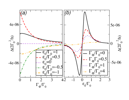
Figure 2: Heat-current asymmetry in the linear regime (a) as a function of the coupling of the probe $\Gamma_{\Phi}/\Gamma_{0}$, and (b) versus the localized level $\varepsilon_{0}/\Gamma_{0}$. Parameters: $E_{F}=0$, $\Gamma_{1}=\Gamma_{2}=\Gamma_{0}/2$, $eV=0.01\Gamma_{0}$, $k_{B}\theta=0.01\Gamma_{0}$.

VI Numerical results

In this section, we present numerical calculations for the heat asymmetries of our two-terminal quantum dot in both linear and nonlinear regimes. In either case, the integrals following from substitution of Eq. (19) in Eqs. (3) and (4) require a careful analysis (see Appendix). We begin with the linear regime. In Fig. 2, we show the heat asymmetry $\Delta=\Delta_{C}=\Delta_{E}$ as a function of the probe coupling $\Gamma_{\Phi}/\Gamma_{0}$ [Fig. 2(a)] and the dot level $\varepsilon_{0}/\Gamma_{0}$, which can be tuned with an external gate voltage [Fig. 2(b)]. We observe in Fig. 2(a) that inelastic processes reduce the heat asymmetry $\Delta$ and that the asymmetry is not a monotonic function of the gate. Due to the probe coupling, the dot transmission acquires an additional level broadening (we recall that $\Gamma=\Gamma_{1}+\Gamma_{2}+\Gamma_{\Phi}$). When $\Gamma_{\Phi}$ increases the dot transmission becomes broader and shows a weaker energy dependence. As a result, the energy current is reduced overall. We notice that $\Delta$ shows electron-hole symmetry, i.e., $\Delta(\varepsilon_{0})=-\Delta(-\varepsilon_{0})$. This fact is more explicit in Fig. 2(b) and is due to the absence of screening effects in the linear regime. Here, the curves $\Delta$ versus the dot level show a resonant-like behavior in which $\Delta$ becomes an extremum for $2|\varepsilon_{0}|/\Gamma\simeq 1$. Additionally, this $\Delta$ extremal point depends quite strongly on $k_{B}\theta$ (not shown here). Indeed, at very low temperatures the value for which $\Delta$ is maximum or minimum indicates the energy scale for which the transmission changes more abruptly around the Fermi energy.

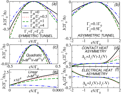
Figure 3: Heat-current characteristic ($\mathcal{J}-V$) for various values of the probe strength $\Gamma_{\Phi}/\Gamma_{0}$ (a) for a symmetric tunnel configuration $\Gamma_{1}=\Gamma_{2}=\Gamma_{0}/2$, and (b) for an asymmetric tunnel configuration $\Gamma_{1}=0.1\Gamma_{0}$, and $\Gamma_{2}=0.9\Gamma_{0}$. (c), and (e) show enlarged parts of $\mathcal{J}-V$ corresponding to the quadratic and linear behavior of the heat current versus voltage, respectively. (d), and (f) illustrate the contact ($\Delta_{C}$), and electrical ($\Delta_{E}$) heat asymmetries. Parameters: $E_{F}=0$, $k_{B}\theta=0.01\Gamma_{0}$, $\varepsilon_{0}/\Gamma_{0}=1$, $C=0$.

In the nonlinear regime, rectification effects arise, as illustrated in Fig. 3. For definiteness, we consider a symmetrically electrical biased quantum dot, i.e., $V_{1}=-V_{2}=V/2$ with a common background temperature $\theta$ for both contacts. This electrical and thermal configuration mimics the experimental conditions reported by Lee et al. in Ref. Lee et al. (2013). We show the heat flow $\mathcal{J}=\mathcal{J}_{1}(V)$ through contact $1$ for a symmetrically coupled quantum dot ($\Gamma_{1}=\Gamma_{2}$) in Fig. 3(a), and for an asymmetric tunnel configuration in Fig. 3(b) ($\Gamma_{1}\neq\Gamma_{2}$). In both cases, we observe rectification effects, $\mathcal{J}(V)\neq-\mathcal{J}(-V)$ even for moderate voltages. These are mainly caused by the Joule heating term, which can be further strengthened by an asymmetric potential response in the case $\Gamma_{1}\neq\Gamma_{2}$ (López and Sánchez, 2013). In fact, as shown in Fig. 3(c), the heat flow becomes a quadratic function of voltage, $\mathcal{J}(V)=M^{(0)}V+M^{(1)}V^{2}$ ($M^{(0)}=M_{11}$ represents the leading-order electrothermal coefficient López and Sánchez (2013)). Thus, $J$ is quickly dominated by the Joule power at low bias $\mathcal{P}_{\rm Joule}=\mathcal{I}V\propto M^{(1)}V^{2}$. For a small-bias range, Fig. 3(e) displays the linear transport regime in which $\mathcal{J}=M^{(0)}V\propto V$ (Peltier effect). We observe that in the strongly nonlinear regime, the effect of increasing $\Gamma_{\Phi}/\Gamma_{0}$ [Figs. 3(a) and 3(b)] causes a decrease of the Peltier and the heat current thus becomes more symmetric under reversal of the bias polarity. The contact and electric heat asymmetries, $\Delta_{C}$ and $\Delta_{E}$, are shown in Figs. 3(d) and (f). We observe that inelastic processes (increasing $\Gamma_{\Phi}/\Gamma_{0}$) reduce the value of $\Delta_{C}$ [Fig. 3(d)] since the contact heat asymmetry $\Delta_{C}$ coincides with the energy current $\mathcal{J}^{E}$ for symmetric biases, as shown in Eq. (21). Hence, by increasing $\Gamma_{\Phi}/\Gamma_{0}$ the transmission acquires a weaker energy dependence, leading to a suppression of the energy current for our device and therefore a decrease of $\Delta_{C}$. The electrical heat asymmetry is, by construction, insensitive to rectification effects, as depicted in Fig. 3(f). Moreover, we also observe a decrease of $\Delta_{E}$ as the amount of incoherent scattering, $\Gamma_{\Phi}/\Gamma_{0}$, increases.

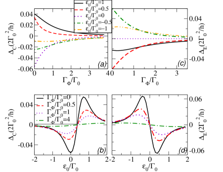
Figure 4: Heat-current asymmetry in the nonlinear regime for an asymmetric tunnel configuration $\Gamma_{1}=0.1\Gamma_{0}$, and $\Gamma_{2}=0.9\Gamma_{0}$. Contact heat asymmetry $\Delta_{C}=J_{1}(V)-J_{2}(V)$: (a) as a function of the coupling of the probe $\Gamma_{\Phi}/\Gamma_{0}$, and (b) versus the localized level $\varepsilon_{0}/\Gamma_{0}$. Electrical heat asymmetry $\Delta_{E}=J_{1}(V)-J_{1}(-V)$: (c) as a function of the probe coupling $\Gamma_{\Phi}/\Gamma_{0}$, and (d) versus the dot level $\varepsilon_{0}/\Gamma_{0}$. Parameters: $E_{F}=0$, $\Gamma_{1}=0.1\Gamma_{0}$, $\Gamma_{2}=0.9\Gamma_{0}$, $eV=\Gamma_{0}$, $k_{B}\theta=0.01\Gamma_{0}$, $C=0$.

Finally, we discuss the behavior of the heat asymmetries with the probe coupling strength $\Gamma_{\Phi}$ and dot level $\varepsilon_{0}$ in Fig. 4 for the nonlinear regime (we set $eV/\Gamma_{0}=1$). The heat-contact asymmetry dependence with $\Gamma_{\Phi}/\Gamma_{0}$ is presented in Fig. 4(a) for different $\varepsilon_{0}/\Gamma_{0}$ values. We observe departures from the electron-hole symmetry, $\Delta_{C}(\varepsilon_{0})\neq-\Delta_{C}(-\varepsilon_{0})$, when the strength of the probe is relatively small, whereas if $\Gamma_{\Phi}/\Gamma_{0}$ becomes larger such effects are removed due to an overall reduction of this heat asymmetry. Figure 4(c) shows the electrical asymmetry, which is electron-hole symmetric by construction. As previously, $\Delta_{E}$ is broadly reduced when $\Gamma_{\Phi}/\Gamma_{0}$ grows. The dot gate dependence of the heat asymmetries, for specific values of $\Gamma_{\Phi}/\Gamma_{0}$, is shown in Figs. 4(b) and (d). In both cases, the heat asymmetries show a peak structure, which is reduced with increasing probe strengths. However, Fig. 4(b) clearly shows the absence of electron-hole symmetry for $\Delta_{C}$.

VII Conclusions

In closing, we have formulated a generic framework for the assessment of inelastic and dephasing processes in the power asymmetry of nanoscale junctions. We have found that in linear response, the heat-current asymmetries (both measured in a given contact or in different electrodes) agree and are given at low temperatures by the energy derivative of a modified transmission function. In the nonlinear regime of transport, both asymmetries differ and present an interesting behavior in terms of the coupling to the dephasing probe and the gate-tunable energy level. Quite generally, the heat asymmetries vanish with an increasing amount of inelasticity or dephasing.

Our results are independent of the microscopic origin of incoherent scattering. Qualitatively, we believe that our main conclusions will be robust and applicable to a large variety of systems. Yet, it would be highly desirable to investigate in future works specific models taking into account, e.g., electron-phonon interactions.

Further extensions of the model should consider cooling effects Galperin et al. (2009), whose efficiency in the nonlinear regime and in the presence of incoherent scattering remains an open issue. Another interesting question, perhaps more fundamental, is the development of magnetic-field asymmetries in multiterminal setups Matthews et al. (2014). It is well known that in the nonlinear regime departures of the Onsager reciprocity are quite general Hwang et al. (2013). The role of inelasticity and decoherence is less clear. Finally, we would like to mention the exciting possibility of implementing rectifying nanojunctions for energy harvesting Sothmann et al. (2015). A deep study of the combined effect of nonlinearities and incoherent scattering would bring the goal of waste-heat–to–electricity nanoconverters closer to reality.

Appendix A Charge and heat current integrals

In our numerical analysis, it is worth to calculate the integral for the charge current through the source electrode,

$$\mathcal{I}_{1}=\frac{2e}{h}\int_{\mathbb{R}}dE\frac{\Gamma_{1}\Gamma_{2}}{\left(E-\epsilon\right)^{2}+\Gamma^{2}/4}[f_{1}(E)-f_{2}(E)]\,,$$ (23)

and the corresponding heat flux,

$$\mathcal{J}_{1} =\frac{2}{h}\int_{\mathbb{R}}dE\left(E-\mu_{1}\right)\frac{\Gamma_{1}\Gamma_{2}}{\left(E-\epsilon\right)^{2}+\Gamma^{2}/4}$$

$$\times[f_{1}(E)-f_{2}(E)]\,.$$ (24)

Here, $\epsilon$ can be $\varepsilon_{0}$ for the linear response or $\varepsilon_{0}+e\mathcal{U}(V,\theta)$ in the nonlinear regime of transport, with $\mathcal{U}$ evaluated self-consistently in terms of the applied voltage $V$ and temperature difference $\theta$.

An analytical solution of Eqs. (23) and (24) can be obtained by noticing that the Fermi functions can be expressed in terms of the digamma function $\Psi(z)=\Gamma^{\prime}(z)/\Gamma\left(z\right)$:

$$f_{j}(E) =\frac{1}{2}\left[1-\tanh{\left(\frac{E-\mu_{j}}{2k_{B}T_{j}}\right)}\right]$$

$$=\frac{1}{2}\left[1+\frac{i}{\pi}\left[\Psi\left(\frac{1}{2}+i\frac{w_{j}(E)}{\pi}\right)-\Psi\left(\frac{1}{2}-i\frac{w_{j}(E)}{\pi}\right)\right]\right]\,,$$ (25)

where $w_{j}(E)=(E-\mu_{j})/(2k_{B}T_{j})$. The first (second) $\Psi$ has singularities at $w_{j}=i\pi\left(n+\frac{1}{2}\right)$ [$w_{j}=-i\pi\left(n+\frac{1}{2}\right)$] with $n\in\mathds{N}$.

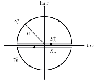
Figure 5: Integration contour in the complex plane.

Consider now the integral

$$I=\int_{\mathbb{R}}dE\,\tau(E)f_{j}(E)=I_{A}+I_{B}+I_{C}\,,$$ (26)

where $\tau(E)=\left[\left(E-\epsilon\right)^{2}+\left(\Gamma/2\right)^{2}\right]^{-1}$ and

$$I_{A} =\frac{1}{2}\int_{\mathbb{R}}dE\,\tau(E)\,,$$ (27)

$$I_{B} =\frac{i}{2\pi}\int_{\mathbb{R}}dE\,\tau(E)\Psi\left(\frac{1}{2}+i\frac{E-\mu_{j}}{2\pi k_{B}T_{j}}\right)\,,$$ (28)

$$I_{C} =-\frac{i}{2\pi}\int_{\mathbb{R}}dE\,\tau(E)\Psi\left(\frac{1}{2}-i\frac{E-\mu_{j}}{2\pi k_{B}T_{j}}\right)\,.$$ (29)

We compute these integrals using the residue theorem. For $I_{A}$ and $I_{C}$ we choose the upper semidisk $S_{R}^{+}$ of radius $R$ while for $I_{B}$ it is convenient to integrate over the lower semidisk $S_{R}^{-}$ (see Fig. 5). In the limit of infinite radius ($R\to\infty$), the integrals along the external paths $\gamma_{R}^{\pm}$ vanish and we find

$$I_{A} =\frac{\pi}{\Gamma}\,,$$ (30)

$$I_{B} =\frac{i}{\Gamma}\Psi\left(\frac{1}{2}+i\frac{\epsilon-\mu_{j}-i\Gamma/2}{2\pi k_{B}T_{j}}\right)\,,$$ (31)

$$I_{C} =-\frac{i}{\Gamma}\Psi\left(\frac{1}{2}-i\frac{\epsilon-\mu_{j}+i\Gamma/2}{2\pi k_{B}T_{j}}\right)\,.$$ (32)

Substituting in Eq. (26) and defining $z_{j}^{\pm}=\left(\frac{1}{2}+\frac{\Gamma}{4\pi k_{B}T_{j}}\pm i\frac{\epsilon-\mu_{j}}{2\pi k_{B}T_{j}}\right)$, Eq. (23) becomes

$$\mathcal{I}_{1}=-\frac{4e}{h}\frac{\Gamma_{1}\Gamma_{2}}{\Gamma}\operatorname{Im}\left[\Psi\left(z_{1}^{+}\right)-\Psi\left(z_{2}^{+}\right)\right]\,,$$ (33)

where we have used the property $\Psi\left(z^{*}\right)=\Psi^{*}\left(z\right)$.

The expression for the heat current [Eq. (24)] is to be treated with caution because in this case there arises a nonzero contribution from the integration along $\gamma_{R}^{\pm}$. Consider

$$J =\int_{\mathbb{R}}dz\left(z-\mu_{1}\right)\tau(z)\left[f_{1}(z)-f_{2}(z)\right]$$

$$=\lim_{R\to\infty}\frac{i}{2\pi}({J_{\gamma_{R}}}-{J_{S}})\,,$$ (34)

with

$$J_{S} =\int_{S_{R}^{-}}dz\left(z-\mu_{1}\right)\tau(z)\left[\Psi_{1}^{+}\left(z\right)-\Psi_{2}^{+}\left(z\right)\right]$$

$$+\int_{S_{R}^{+}}dz\left(z-\mu_{1}\right)\tau(z)\left[\Psi_{1}^{-}\left(z\right)-\Psi_{2}^{-}\left(z\right)\right]\,,$$ (35)

$${J_{\gamma_{R}}} =\int_{\gamma_{R}^{-}}dz\left(z-\mu_{1}\right)\tau(z)\left[\Psi_{1}^{+}\left(z\right)-\Psi_{2}^{+}\left(z\right)\right]$$

$$+\int_{\gamma_{R}^{+}}dz\left(z-\mu_{1}\right)\tau(z)\left[\Psi_{1}^{-}\left(z\right)-\Psi_{2}^{-}\left(z\right)\right]\,.$$ (36)

Here, $\Psi_{j}^{\pm}\left(z\right)=\Psi\left(\frac{1}{2}\pm i\frac{z-\mu_{j}}{2\pi k_{B}T_{j}}\right)$ and the paths $S_{R}^{\pm}$, $\gamma_{R}^{\pm}$ are crossed anticlockwise. $J_{S}$ can be obtained analogously to the charge current case:

$$J_{S} =\frac{4\pi i}{\Gamma}\left(\epsilon-\mu_{1}\right)\operatorname{Im}\left[\Psi_{1}^{+}\left(z\right)-\Psi_{2}^{+}\left(z\right)\right]$$

$$-2\pi i\operatorname{Re}\left[\Psi_{1}^{+}\left(z\right)-\Psi_{2}^{+}\left(z\right)\right]\,.$$ (37)

To compute ${J_{\gamma_{R}}}=J_{\gamma_{R}^{-}}+J_{\gamma_{R}^{+}}$, we use the polar representation $z=Re^{i\theta}$,

$$J_{{\gamma}_{R}^{\pm}} =\int_{0}^{\pi}d\theta\frac{iRe^{i\theta}\left(Re^{i\theta}\mp\mu_{1}\right)}{\left(Re^{i\theta}\mp\epsilon\right)^{2}+\Gamma^{2}/4}$$

$$\times\left[\Psi\left(\frac{1}{2}+i\frac{-Re^{i\theta}\pm\mu_{1}}{2\pi k_{B}T_{1}}\right)-\Psi\left(\frac{1}{2}+i\frac{-Re^{i\theta}\pm\mu_{2}}{2\pi k_{B}T_{2}}\right)\right]\,.$$ (38)

Let $g_{\pm}\left(R,\theta\right)$ be the function under the integral of Eq. (A). For $\left|z\right|\to\infty$ we use the asymptotic value $\Psi\left(z\right)\to\ln\left(z\right)$. As a consequence, for every $\theta\in\left(0,\pi\right)$ one has $g_{\pm}\left(R,\theta\right)\underset{R\to\infty}{\longrightarrow}i\ln{(T_{2}/T_{1})}$. Thus,

$$\lim_{R\to\infty}J_{{\gamma}_{R}^{\pm}}=\pi i\ln\frac{T_{2}}{T_{1}}.$$ (39)

Collecting Eqs. (37) and (39) in Eq. (24), we finally obtain the analytical expression for the heat current:

$$\mathcal{J}_{1} =-\frac{4\Gamma_{1}\Gamma_{2}}{h\Gamma}\left(\epsilon-\mu_{1}\right)\operatorname{Im}\left[\Psi\left(z_{1}^{+}\right)-\Psi\left(z_{2}^{+}\right)\right]$$

$$+\frac{2\Gamma_{1}\Gamma_{2}}{h}\operatorname{Re}\left[\Psi\left(z_{1}^{+}\right)-\Psi\left(z_{2}^{+}\right)\right]-\frac{2\Gamma_{1}\Gamma_{2}}{h}\ln\frac{T_{2}}{T_{1}}.$$ (40)

References

- Sánchez and Linke (2014) D. Sánchez and H. Linke, Focus on thermoelectric effects in nanostructures, New. J. Phys. 16, 110201 (2014), and references cited therein.
- Kim et al. (2012) K. Kim, W. Jeong, W. Lee, and P. Reddy, Ultra-high vacuum scanning thermal microscopy for nanometer resolution quantitative thermometry, ACS Nano 6, 4248 (2012).
- Shakouri (2006) A. Shakouri, Nanoscale thermal transport and microrefrigerators on a chip, IEEE 94, 1613 (2006).
- Giazotto et al. (2006) F. Giazotto, T. T. Heikkilä, A. Luukanen, A. M. Savin, and J. P. Pekola, Opportunities for mesoscopics in thermometry and refrigeration: Physics and applications, Rev. Mod. Phys. 78, 217 (2006).
- Terraneo et al. (2002) M. Terraneo, M. Peyrard, and G. Casati, Controlling the energy flow in nonlinear lattices: a model for a thermal rectifier, Phys. Rev. Lett. 88, 094302 (2002).
- Heremans et al. (2013) J. P. Heremans, M. S. Dresselhaus, L. E. Bell, and D. T. Morelli, When thermoelectrics reached the nanoscale, Nature Nanotech. 8, 471 (2013).
- Snyder and Toberer (2008) G. J. Snyder and E. S. Toberer, Complex thermoelectric materials, Nature Mater. 7, 105 (2008).
- Li et al. (2010) J.-F. Li, W.-S. Liu, L.-D. Zhao, and M. Zhou, High-performance nanostructured thermoelectric materials, NPG Asia Materials 2, 152 (2010).
- Jezouin et al. (2013) S. Jezouin, F. D. Parmentier, A. Anthore, U. Gennser, A. Cavanna, Y. Jin, and F. Pierre, Quantum limit of heat flow across a single electronic channel, Science 342, 601 (2013).
- Molenkamp et al. (1992) L. W. Molenkamp, T. Gravier, H. van Houten, O. J. A. Buijk, M. A. A. Mabesoone, and C. T. Foxon, Peltier coefficient and thermal conductance of a quantum point contact, Phys. Rev. Lett. 68, 3765 (1992).
- Kane et al. (1997) C. Kane, L. Balents, and M. P. A. Fisher, Coulomb interactions and mesoscopic effects in carbon nanotubes, Phys. Rev. Lett. 79, 5086 (1997).
- Battista et al. (2013) F. Battista, M. Moskalets, M. Albert, and P. Samuelsson, Quantum heat fluctuations of single-particle sources, Phys. Rev. Lett. 110, 126602 (2013).
- Spilla et al. (2014) S. Spilla, F. Hassler, and J. Splettstoesser, Measurement and dephasing of a flux qubit due to heat currents, New. J. Phys. 16, 045020 (2014).
- Lee et al. (2013) W. Lee, K. Kim, W. Jeong, L. A. Zotti, F. Pauly, J. C. Cuevas, and P. Reddy, Heat dissipation in atomic-scale junctions, Nature (London) 498, 209 (2013).
- Zotti et al. (2014) L. A. Zotti, M. Bürkle, F. Pauly, W. Lee, K. Kim, W. Jeong, Y. Asai, P. Reddy, and J. C. Cuevas, Heat dissipation and its relation to thermopower in single-molecule junctions, New. J. Phys. 16, 015004 (2014).
- Paulsson and Datta (2003) M. Paulsson and S. Datta, Thermoelectric effect in molecular electronics, Phys. Rev. B 67, 241403 (2003).
- Frederiksen et al. (2004) T. Frederiksen, M. Brandbyge, N. Lorente, and A.-P. Jauho, Inelastic scattering and local heating in atomic gold wires, Phys. Rev. Lett. 93, 256601 (2004).
- Koch et al. (2004) J. Koch, F. von Oppen, Y. Oreg, and E. Sela, Thermopower of single-molecule devices, Phys. Rev. B 70, 195107 (2004).
- Galperin et al. (2007) M. Galperin, A. Nitzan, and M. A. Ratner, Heat conduction in molecular transport junctions, Phys. Rev. B 75, 155312 (2007).
- Finch et al. (2009) C. M. Finch, V. M. García-Suárez, and C. J. Lambert, Giant thermopower and figure of merit in single-molecule devices, Phys. Rev. B 79, 033405 (2009).
- Entin-Wohlman and Aharony (2012) O. Entin-Wohlman and A. Aharony, Three-terminal thermoelectric transport under broken time-reversal symmetry, Phys. Rev. B 85, 085401 (2012).
- Zimbovskaya (2014) N. A. Zimbovskaya, The effect of dephasing on the thermoelectric efficiency of molecular junctions, J. Phys.: Condens. Matter 26, 275303 (2014).
- Büttiker (1988) M. Büttiker, Coherent and sequential tunneling in series barriers, IBM J. Res. Dev. 32, 63 (1988).
- D’Amato and Pastawski (1990) J. L. D’Amato and H. M. Pastawski, Conductance of a disordered linear chain including inelastic scattering events, Phys. Rev. B 41, 7411 (1990).
- de Jong and Beenakker (1996) M. J. M. de Jong and C. W. J. Beenakker, Semiclassical theory of shot noise in mesoscopic conductors, Physica A 230, 219 (1996).
- van Langen and Büttiker (1997) S. A. van Langen and M. Büttiker, Quantum-statistical current correlations in multilead chaotic cavities, Phys. Rev. B 56, R1680 (1997).
- Saito et al. (2011) K. Saito, G. Benenti, G. Casati, and T. Prosen, Thermopower with broken time-reversal symmetry, Phys. Rev. B 84, 201306 (2011).
- Sánchez and Serra (2011) D. Sánchez and L. Serra, Thermoelectric transport of mesoscopic conductors coupled to voltage and thermal probes, Phys. Rev. B 84, 201307 (2011).
- Caso et al. (2012) A. Caso, L. Arrachea, and G. S. Lozano, Defining the effective temperature of a quantum driven system from current-current correlation functions, Eur. Phys. J. B 85, 1 (2012).
- Bedkihal et al. (2013) S. Bedkihal, M. Bandyopadhyay, and D. Segal, The probe technique far from equilibrium: Magnetic field symmetries of nonlinear transport, Eur. Phys. J. B 86, 1 (2013).
- Bergfield et al. (2013) J. P. Bergfield, S. M. Story, R. C. Stafford, and C. A. Stafford, Probing Maxwell’s demon with a nanoscale thermometer, ACS Nano 7, 4429 (2013).
- Apertet et al. (2013) Y. Apertet, H. Ouerdane, C. Goupil, and P. Lecoeur, From local force-flux relationships to internal dissipations and their impact on heat engine performance: The illustrative case of a thermoelectric generator, Phys. Rev. E 88, 022137 (2013).
- Brandner and Seifert (2013) K. Brandner and U. Seifert, Multi-terminal thermoelectric transport in a magnetic field: bounds on Onsager coefficients and efficiency, New. J. Phys. 15, 105003 (2013).
- Meair et al. (2014) J. Meair, J. P. Bergfield, C. A. Stafford, and P. Jacquod, Local temperature of out-of-equilibrium quantum electron systems, Phys. Rev. B 90, 035407 (2014).
- Butcher (1990) P. N. Butcher, Thermal and electrical transport formalism for electronic microstructures with many terminals, J. Phys.: Condens. Matter 2, 4869 (1990).
- Christen and Büttiker (1996) T. Christen and M. Büttiker, Gauge-invariant nonlinear electric transport in mesoscopic conductors, EPL 35, 523 (1996).
- Sánchez and López (2013) D. Sánchez and R. López, Scattering theory of nonlinear thermoelectric transport, Phys. Rev. Lett. 110, 026804 (2013).
- Meair and Jacquod (2013) J. Meair and P. Jacquod, Scattering theory of nonlinear thermoelectricity in quantum coherent conductors, J. Phys.: Condens. Matter 25, 082201 (2013).
- Cutler and Mott (1969) M. Cutler and N. F. Mott, Observation of Anderson localization in an electron gas, Phys. Rev. 181, 1336 (1969).
- Jonson and Mahan (1980) M. Jonson and G. D. Mahan, Mott’s formula for the thermopower and the Wiedemann-Franz law, Phys. Rev. B 21, 4223 (1980).
- Meir and Wingreen (1992) Y. Meir and N. S. Wingreen, Landauer formula for the current through an interacting electron region, Phys. Rev. Lett. 68, 2512 (1992).
- Staring et al. (1993) A. A. M. Staring, L. W. Molenkamp, B. W. Alphenaar, H. van Houten, O. J. A. Buyk, M. A. A. Mabesoone, C. W. J. Beenakker, and C. T. Foxon, Coulomb-blockade oscillations in the thermopower of a quantum dot, EPL 22, 57 (1993).
- Svensson et al. (2013) S. F. Svensson, E. A. Hoffmann, N. Nakpathomkun, P. M. Wu, H. Q. Xu, H. A. Nilsson, D. Sánchez, V. Kashcheyevs, and H. Linke, Nonlinear thermovoltage and thermocurrent in quantum dots, New. J. Phys. 15, 105011 (2013).
- Sierra and Sánchez (2014) M. A. Sierra and D. Sánchez, Strongly nonlinear thermovoltage and heat dissipation in interacting quantum dots, Phys. Rev. B 90, 115313 (2014).
- Kulik (1994) I. O. Kulik, Non-linear thermoelectricity and cooling effects in metallic constrictions, J. Phys.: Condens. Matter 6, 9737 (1994).
- Bogachek et al. (1999) E. N. Bogachek, A. G. Scherbakov, and U. Landman, Nonlinear Peltier effect and thermoconductance in nanowires, Phys. Rev. B 60, 11678 (1999).
- Li et al. (2004) B. Li, L. Wang, and G. Casati, Thermal diode: rectification of heat flux, Phys. Rev. Lett. 93, 184301 (2004).
- Segal (2006) D. Segal, Heat flow in nonlinear molecular junctions: Master equation analysis, Phys. Rev. B 73, 205415 (2006).
- Ruokola et al. (2009) T. Ruokola, T. Ojanen, and A.-P. Jauho, Thermal rectification in nonlinear quantum circuits, Phys. Rev. B 79, 144306 (2009).
- Kuo and Chang (2010) D. M.-T. Kuo and Y.-C. Chang, Thermoelectric and thermal rectification properties of quantum dot junctions, Phys. Rev. B 81, 205321 (2010).
- Whitney (2013) R. S. Whitney, Nonlinear thermoelectricity in point contacts at pinch off: A catastrophe aids cooling, Phys. Rev. B 88, 064302 (2013).
- López and Sánchez (2013) R. López and D. Sánchez, Nonlinear heat transport in mesoscopic conductors: Rectification, Peltier effect, and Wiedemann-Franz law, Phys. Rev. B 88, 045129 (2013).
- Hwang et al. (2013) S.-Y. Hwang, D. Sánchez, M. Lee, and R. López, Magnetic-field asymmetry of nonlinear thermoelectric and heat transport, New. J. Phys. 15, 105012 (2013).
- Whitney (2014) R. S. Whitney, Most efficient quantum thermoelectric at finite power output, Phys. Rev. Lett. 112, 130601 (2014).
- Utsumi et al. (2014) Y. Utsumi, O. Entin-Wohlman, A. Aharony, T. Kubo, and Y. Tokura, Fluctuation theorem for heat transport probed by a thermal probe electrode, Phys. Rev. B 89, 205314 (2014).
- Werlang et al. (2014) T. Werlang, M. A. Marchiori, M. F. Cornelio, and D. Valente, Optimal rectification in the ultrastrong coupling regime, Phys. Rev. E 89, 062109 (2014).
- Eich et al. (2014) F. G. Eich, A. Principi, M. Di Ventra, and G. Vignale, Luttinger-field approach to thermoelectric transport in nanoscale conductors, Phys. Rev. B 90, 115116 (2014).
- Gergs et al. (2014) N. M. Gergs, C. B. M. H rig, M. R. Wegewijs, and D. Schuricht, Charge fluctuations in nonlinear heat transport, arXiv:1407.8284 (preprint) (2014).
- Biele et al. (2014) R. Biele, R. D’Agosta, and A. Rubio, Time-dependent thermal transport theory, arXiv:1412.5765 (preprint) (2014).
- Cuevas and Scheer (2010) J. C. Cuevas and E. Scheer, Molecular electronics: an introduction to theory and experiment (World Scientific, 2010).
- Galperin et al. (2009) M. Galperin, K. Saito, A. V. Balatsky, and A. Nitzan, Cooling mechanisms in molecular conduction junctions, Phys. Rev. B 80, 115427 (2009).
- Matthews et al. (2014) J. Matthews, F. Battista, D. Sánchez, P. Samuelsson, and H. Linke, Experimental verification of reciprocity relations in quantum thermoelectric transport, Phys. Rev. B 90, 165428 (2014).
- Sothmann et al. (2015) B. Sothmann, R. Sánchez, and A. N. Jordan, Thermoelectric energy harvesting with quantum dots, Nanotechnology 26, 032001 (2015).