Robust estimation of mixtures of regressions with random covariates, via trimming and constraints

Abstract

A robust estimator for a wide family of mixtures of linear regression is presented. Robustness is based on the joint adoption of the Cluster Weighted Model and of an estimator based on trimming and restrictions. The selected model provides the conditional distribution of the response for each group, as in mixtures of regression, and further supplies local distributions for the explanatory variables. A novel version of the restrictions has been devised, under this model, for separately controlling the two sources of variability identified in it. This proposal avoids singularities in the log-likelihood, caused by approximate local collinearity in the explanatory variables or local exact fits in regressions, and reduces the occurrence of spurious local maximizers. In a natural way, due to the interaction between the model and the estimator, the procedure is able to resist the harmful influence of bad leverage points along the estimation of the mixture of regressions, which is still an open issue in the literature. The given methodology defines a well-posed statistical problem, whose estimator exists and is consistent to the corresponding solution of the population optimum, under widely general conditions. A feasible EM algorithm has also been provided to obtain the corresponding estimation. Many simulated examples and two real datasets have been chosen to show the ability of the procedure, on the one hand, to detect anomalous data, and, on the other hand, to identify the real cluster regressions without the influence of contamination.

1 Introduction

Mixture models provide a quite flexible approach to statistical modeling of a wide variety of random phenomena, whenever we can reasonably suppose that the observations arise from unobserved groups in the population. Under this general framework, the present paper provides a new proposal in the family of finite mixtures of robust regressions (DeSarbo and Cron, 1988; de Veaux, 1989).

Assume we are provided with two quantitative random variables $\mathbf{X}$ and $Y$: $\mathbf{X}$ is a vector of explanatory variables, $Y$ is a response or outcome variable, and the dependence between $Y$ and $\mathbf{X}$ may vary among the different underlying groups. By adopting the cluster-weighted approach, we allow different scatter structures in each group, both in the marginal distribution of $\mathbf{X}$ and in the conditional distribution of $Y|\mathbf{X}=\mathbf{x}$, as it is required by many observed dataset. The Cluster Weighted Model (CWM), introduced in Gershenfeld (1997), decomposes the joint p.d.f. of $(\mathbf{X},Y)$ in each component of the mixture as the product of the marginal and the conditional distributions.

Due to its very definition, the CWM estimator is able to take into account different distributions for the explanatory variables across groups, so overcoming an intrinsic limitation of mixtures of regression, where they are implicitly assumed equally distributed. However, due to the possible presence of contaminating data (background noise, pointwise contamination, unexpected minority patterns, etc.) a small fraction of outliers could severely affect the model fitting. Among the available standard techniques in robust estimation, those based on removing part of the data - and called impartial trimming procedures - present a good performance, often being an obligatory benchmark to compare new estimators. Successful robust procedures of this kind are, for instance, the LTS for regression models (Rousseeuw and Leroy, 1987), the trimmed k-means (Cuesta-Albertos et al., 1997), the TCLUST for clustering (García-Escudero et al., 2008), and the robust clusterwise linear regression models (García-Escudero et al., 2010). Here, in the framework of mixtures of regressions, denoting by $\mathbf{x}$ and $y$ the realizations of $\mathbf{X}$ and $Y$, standard diagnostic tools can easily identify outliers on $y$ that fall in the range of values of $\mathbf{x}$, while the detection of outliers on both $\mathbf{x}$ and $y$, that may act as bad leverage points, is much more problematic. Many trimming approaches are effective for the first type of outliers, but they fail when dealing with bad leverage points. In this paper, we exploit the CWM nice feature of modeling the $\mathbf{X}$ marginal distribution, to detect dangerous outliers on $\mathbf{x}$. At the same time, we also use the regression structure among $\mathbf{X}$ and $Y$ to deal with outliers on $y$. In this way, by robustifying the CWM estimation, we can simultaneously handle both type of outliers with the same formal approach. As usual when using trimming, only the total fraction of discarded observations must be fixed in advance.

A further issue with ML estimation for CWMs is the unboundedness of the log-likelihood function, a well-known aspect pointed out in Day (1969) for Gaussian mixtures. To overcome this drawback, Hathaway (1985) introduced the use of constrained variance estimation in univariate mixture modeling. These restrictions have been extended to the multivariate case in different ways by McLachlan and Peel (2004), Ingrassia and Rocci (2007) and García-Escudero et al. (2008). By adopting restrictions also for CWM, we arrive at setting a well-posed optimization problem. Additionally, a restricted approach not only avoids singularities, it also discards non-interesting local maximizers of the objective function (García-Escudero et al., 2014b). We will discuss in detail how approximate local collinearity in the explanatory variables, and approximate local exact fits in the regressions may cause, indeed, serious troubles in CWMs.

The above considerations give rise to the robust estimation of the trimmed Cluster Weighted Restricted Model (trimmed CWRM) presented hereafter. It includes an original application of the constraints, which takes into account the specific features of CWM and controls the relative variability between components for the sources of variability in the model corresponding to: i) the explanatory variables, and ii) the regression errors. The CWM, endowed with restrictions and trimming, becomes a very competitive robust estimator for mixtures of multiple regression, with optimal statistical properties.

We have organized the paper as follows. In Section 2 we recall the main ideas about the CWM. In Section 3 we present the trimmed CWRM, and introduce a feasible algorithm for its practical implementation. Then, we state the central findings of the paper, i.e. the existence and the strong consistency of the new estimator. Section 4 provides a discussion on the effects of constraints and trimming, along with some illustrative examples. The application of the proposed methodology to two real data sets is shown in Section 5. Finally, Section 6 contains some concluding remarks and sketches future research. Proofs and technical lemmas needed for our main results are relegated in the Appendix.

2 Cluster Weighted Modeling

The Cluster Weighted Model (CWM) has been proposed in the context of media technology, to build a digital violin with traditional inputs and realistic sounds (Gershenfeld, 1997; Gershenfeld et al., 1999); in Wedel (2000). CWMs are referred to as the family of saturated mixture regression models. In Ingrassia et al. (2012), CWMs have been reformulated in a statistical setting showing that they are a general and flexible family of mixture models. In fact, Ingrassia et al. (2012) show that Gaussian CWM includes, as special cases, finite mixtures of distributions and finite Mixtures of Regression models.

Let $(\mathbf{X},Y)$ be a pair of random variables, namely a vector of covariates $\mathbf{X}$ and a response variable $Y$ defined on $\Omega$ with values in $\mathcal{X}\times\mathcal{Y}\subseteq\mathbb{R}^{d}\times\mathbb{R}$ and $\{(\mathbf{x}_{i},y_{i})\}_{i=1}^{n}$ represents a i.i.d. random sample of size $n$, drawn from $(\mathbf{X},Y)$. Let $p(\mathbf{x},y)$ denote the joint density of $\left(\mathbf{X},Y\right)$, and suppose that $\Omega$ can be partitioned into $G$ groups, say $\Omega_{1},\ldots,\Omega_{G}$. CWMs are mixture models having density of the form

$$p(\mathbf{x},y;\mbox{\boldmath$\theta$})=\sum^{G}_{g=1}p(y|\mathbf{x};\mbox{\boldmath$\xi$}_{g})p(\mathbf{x};\mbox{\boldmath$\psi$}_{g})\pi_{g},$$ (1)

where $p(y|\mathbf{x};\mbox{\boldmath$\xi$}_{g})$ is the conditional density of $Y$ given $\mathbf{x}$ in $\Omega_{g}$ (depending on some parameter $\mbox{\boldmath$\xi$}_{g}$), $p(\mathbf{x};\mbox{\boldmath$\psi$}_{g})$ is the marginal density of $\mathbf{X}$ in $\Omega_{g}$ (depending on some parameter $\mbox{\boldmath$\psi$}_{g}$) and $\pi_{g}$ is the weight of $\Omega_{g}$ in the mixture (with $\pi_{g}>0$ and $\sum_{g=1}^{G}\pi_{g}=1$). Furthermore, we assume that in each group $\Omega_{g}$, the conditional expectation of $Y$ given $\mathbf{X}=\mathbf{x}$, is a function $m(\cdot)$ of $\mathbf{x}$ depending on some parameters $\mbox{\boldmath$\beta$}_{g}$, that is $E(Y|\mathbf{x},\Omega_{g})=m(\mathbf{x};\mbox{\boldmath$\beta$}_{g})$.

In this work, we have focused on models of type (1) with Gaussian components. Thus $p(\mathbf{x};\mbox{\boldmath$\psi$}_{g})=\phi_{d}(\mathbf{x};\mbox{\boldmath$\mu$}_{g},\mbox{\boldmath$\Sigma$}_{g})$, where $\phi_{d}(\cdot;\mbox{\boldmath$\mu$}_{g},\mbox{\boldmath$\Sigma$}_{g})$ denotes the density of the $d$-variate Gaussian distribution with mean vector $\mbox{\boldmath$\mu$}_{g}$ and covariance matrix $\mbox{\boldmath$\Sigma$}_{g}$. Moreover, we have assumed that the conditional relationship between $Y$ and $\mathbf{x}$ in the $g$-th group can be written as $Y=\mathbf{b}_{g}^{\prime}\mathbf{x}+b_{g}^{0}+\varepsilon_{g}$ where $\varepsilon_{g}\sim N(0,\sigma_{g}^{2})$. Hence, $\mathbf{X}|\Omega_{g}\sim N_{d}(\mbox{\boldmath$\mu$}_{g},\mbox{\boldmath$\Sigma$}_{g})$ and $Y|\mathbf{x},\Omega_{g}\sim N(\mathbf{b}^{\prime}_{g}\mathbf{x}+b_{g}^{0},\sigma_{g}^{2})$, so that model (1) specializes to:

$$p(\mathbf{x},y;\mbox{\boldmath$\theta$})=\sum_{g=1}^{G}\phi(y;\mathbf{b}^{\prime}_{g}\mathbf{x}+b_{g}^{0},\sigma_{g})\phi_{d}(\mathbf{x};\mbox{\boldmath$\mu$}_{g},\mbox{\boldmath$\Sigma$}_{g})\pi_{g},$$ (2)

which defines the linear Gaussian CWM. We notice here that definition (2) corresponds to a mixture of regressions, with weights $\phi_{d}(\mathbf{x};\mbox{\boldmath$\mu$}_{g},\mbox{\boldmath$\Sigma$}_{g})\pi_{g}$ depending also on the covariate distributions in each component $g$ for $g=1,\ldots,G$. Finally, in the framework of model-based clustering, each unit is assigned to one group, based on the maximum a posteriori probability. The consideration of (2) yields to the use of (log-)likelihood target function to be maximized as

$$\sum_{i=1}^{n}\log\left[\sum_{g=1}^{G}\phi(y_{i};\mathbf{b}^{\prime}_{g}\mathbf{x}_{i}+b_{g}^{0},\sigma_{g}^{2})\phi_{d}(\mathbf{x}_{i};\mbox{\boldmath$\mu$}_{g},\mbox{\boldmath$\Sigma$}_{g})\pi_{g}\right].$$ (3)

For sake of simplicity, we will later use the notation

$$D_{g}(\mathbf{x},y;\mbox{\boldmath$\theta$})=\phi(y;\mathbf{b}^{\prime}_{g}\mathbf{x}+b_{g}^{0},\sigma_{g}^{2})\phi_{d}(\mathbf{x};\mbox{\boldmath$\mu$}_{g},\mbox{\boldmath$\Sigma$}_{g})\pi_{g}$$

and $D(\mathbf{x},y;\mbox{\boldmath$\theta$})\allowbreak=\sum_{g=1}^{G}D_{g}(\mathbf{x},y;\mbox{\boldmath$\theta$})$, where the set of all parameters of the model is denoted by $\theta$, and, such that (3) is simply rewritten as $\sum_{i=1}^{n}\log[D(\mathbf{x}_{i},y_{i};\mbox{\boldmath$\theta$})]$. Additionally, the linear Gaussian CWM will be many times simply referred to as CWM.

2.1 Two problems about CWM

The estimation of the (linear Gaussian) CWM suffers from a serious lack of robustness, like it happens when using many other models based on normal assumptions and fitted through ML estimators (see, e.g., Huber, 1981). It is very important to be aware of this issue, due to the common presence of noise sources in data. To illustrate this problem, a simulated data set of $n=180$ units (referred to as Simdata1 hereafter), has been generated from the CWM with $G=2$ and 90 observations from each component. Then we added 20 contaminating observations as either background noise, see Figure 1(a), or pointwise contamination around the point $(15,20)$, see Figure 1(b). The true underlying regression lines (prior to contamination) are represented with dotted lines, and we can see the dangerous effects of outliers on model fitting for the standard CWM.

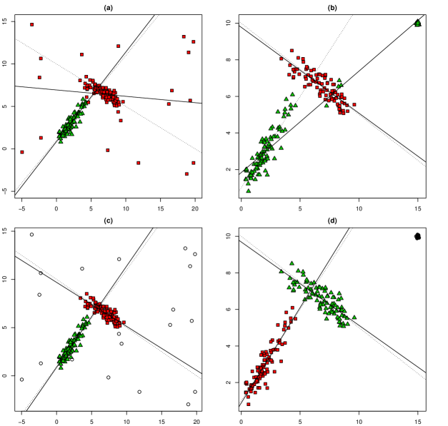
Figure 1: Simdata1: (a) original data plus background noise and CWM fitted; (b) original data plus pointwise contamination and CWM fitted; (c) and (d) show the fitted trimmed CWRMs with $\alpha=0.1$, $c_{X}=c_{\varepsilon}=20$ to these two data sets. The dotted lines represent the true regression lines to be estimated and black circles are the trimmed observations (here and in all the figures).

Another important issue concerns the unboundedness of the target function in (3) when no constraints are imposed on the scatter parameters. In this case, the defining problem is ill-posed because the loglikelihood in (3) tends to $\infty$ when either $\mbox{\boldmath$\mu$}_{g}=\mathbf{x}_{i}$ and $|\mbox{\boldmath$\Sigma$}_{g}|\rightarrow 0$ or $y_{i}=\mathbf{b}^{\prime}_{g}\mathbf{x}_{i}+b_{g}^{0}$ and $\sigma_{g}^{2}\rightarrow 0$. Moreover, as a trivial consequence, the EM algorithms often applied to fit a CWM can be trapped into non-interesting local maximizers, called “spurious” solutions, and the result of the EM algorithm strongly depends on its initialization.

Spurious solutions may be due to very localized patterns in the explanatory variables, as shown in Figure 2(a), by considering a second simulated data set (Simdata2). Here, data concern $n=200$ observations and $d=2$ explanatory variables. The dataset has been built as follows: two sets of 90 observations for the explanatory variable $\mathbf{X}$ has been drawn from two bivariate normal distributions, centered at $(2,2)$ and $(4,4)$, respectively. Then, 20 almost collinear observations have been added to the sample, close to the second component. The values for the response variable $Y$ have been generated by using the same linear function (for both components) with equally distributed error terms. We can see in Figure 2(a) that the standard fit of the CWM yields to the determination of a first spurious component with the 20 almost collinear observations and a second component joining together the two groups, with $90\%$ of the observations.

Sometimes spurious solutions may be also due to localized patterns of observations, where an approximate “exact fit” for a small number of observations can be obtained. Figure 3 shows a third simulated data set (Simdata3) with $n=200$ observations, where 196 of them have been generated from a CWM with $G=2$ components (98 observations from each component). A very small fraction of almost collinear units (only 4 observations) on the $(\mathbf{X},Y)$ variables have been added, with a roughly equal value (around $0$) for the response variable. These values, for instance, could be due to a bad performance of the tool used to measure the response variable. It may be seen that a fitted component including only these almost collinear observations could arise, along the EM estimation, because a small value of one of the $\sigma_{g}^{2}$ parameters yields to higher values of the log-likelihood. Then, the two main linear structures accounting for $98\%$ of the data points would be artificially joined together.

To overcome the previous issues, in the next section we propose a robust methodology by incorporating trimming and constraints to the CWM.

3 Trimmed Cluster Weighted Restricted Modeling

3.1 Problem statement

For a given sample of $n$ observations, the trimmed CWRM methodology is based on the maximization of the following log-likelihood function

$$\sum_{i=1}^{n}z(\mathbf{x}_{i},y_{i})\log\left[\sum_{g=1}^{G}\phi(y_{i};\mathbf{b}^{\prime}_{g}\mathbf{x}_{i}+b_{g}^{0},\sigma_{g}^{2})\phi_{d}(\mathbf{x}_{i};\mbox{\boldmath$\mu$}_{g},\mbox{\boldmath$\Sigma$}_{g})\pi_{g}\right],$$ (4)

where $z(\cdot,\cdot)$ is a 0-1 trimming indicator function that tell us whether observation $(\mathbf{x}_{i},y_{i})$ is trimmed off ($z(\mathbf{x}_{i},y_{i})$=0), or not ($z(\mathbf{x}_{i},y_{i})$=1). A fixed fraction $\alpha$ of observations can be unassigned by setting $\sum_{i=1}^{n}z(\mathbf{x}_{i},y_{i})=[n(1-\alpha)]$. Hence the parameter $\alpha$ denotes the trimming level. Analogous approaches based on trimmed mixture likelihoods can be found in Neykov et al. (2007), Gallegos and Ritter (2009) and García-Escudero et al. (2014b).

Moreover, we introduce two further constraints on the maximization in (4). The first one concerns the set of eigenvalues $\{\lambda_{l}(\mbox{\boldmath$\Sigma$}_{g})\}_{l=1,...,d}$ of the scatter matrices $\mbox{\boldmath$\Sigma$}_{g}$ by imposing

$$\lambda_{l_{1}}(\mbox{\boldmath$\Sigma$}_{g_{1}})\leq c_{X}\lambda_{l_{2}}(\mbox{\boldmath$\Sigma$}_{g_{2}})\quad\quad\text{ for every }1\leq l_{1}\neq l_{2}\leq d\text{ and }1\leq g_{1}\neq g_{2}\leq G.$$ (5)

The second constraint refers to the variances $\sigma_{g}^{2}$ of the regression error terms, by requiring

$$\sigma_{g_{1}}^{2}\leq c_{\varepsilon}\sigma_{g_{2}}^{2}\quad\quad\text{ for every }1\leq g_{1}\neq g_{2}\leq G.$$ (6)

The constants $c_{X}$ and $c_{\varepsilon}$, in (5) and (6) respectively, are finite (not necessarily equal) real numbers, such that $c_{X}\geq 1,c_{\varepsilon}\geq 1$. They automatically guarantee that we are avoiding the $|\mbox{\boldmath$\Sigma$}_{g}|\rightarrow 0$ and $\sigma_{g}^{2}\rightarrow 0$ cases. These constraints are an extension to CWMs of those introduced in Ingrassia and Rocci (2007), García-Escudero et al. (2008) and Greselin and Ingrassia (2010) and go back to Hathaway (1985). The main difference is the asymmetric and different treatment given by the constraints, when modeling the marginal distribution $\mathbf{X}$ or when modeling the regression error terms, providing high flexibility to the model.

Let us consider now the effects of trimming in the two data sets derived from Simdata1. In Figure 1(c) and (d) we can see that setting $\alpha=0.1$ allows to restore the true structure of the data, by discarding the outlying observations, both in the case of background noise and pointwise contamination. Hence, trimming modifies the ML estimation in such a way that it is no more influenced by potential outliers and drives it far from the previous bad results.

Commenting the use of constraints, we can see how a moderate choice of $c_{X}$ for Simdata2 in Figure 2(b) allows to correctly detect the $G=2$ main groups and to avoid the disturbing effect of the spurious patterns in the explanatory variables.

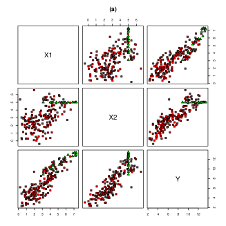
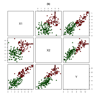
Figure 2: Simdata2: Scatter plot matrix. (a) Almost collinear observations in the explanatory variables which are found as a cluster by CWM when $G=2$; (b) Results of fitting the trimmed CWRM with $\alpha=0$, $c_{X}=c_{\varepsilon}=20$.

Additionally, we can see that a moderate choice of $c_{\varepsilon}$ for Simdata3 would also allow to correctly detect the $G=2$ main groups. Moreover, we can see in Figure 3(a) how only considering $\alpha=0.02$ trimming level (trying to discard the 4 outlying observations in Simdata3) does not solve the problem at all without the consideration of a moderate value of $c_{\varepsilon}$.

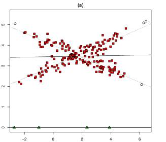
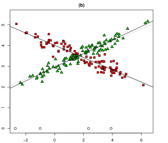
Figure 3: Simdata3: (a) Results of the trimmed CWRM fit with $G=2$, $\alpha=0.02$ and $c_{\varepsilon}=10^{10}$ (almost unrestricted) showing the detection of a spurious component due to an approximate “local exact fit” in one of the fitted regressions; (b) results with $\alpha=0.02$, $c_{X}=c_{\varepsilon}=20$.

A detailed discussion about the role played by $\alpha$, $c_{X}$ and $c_{\varepsilon}$ is given in Section 4.

3.2 Theoretical results

The problem stated in Section 3.1 admits a population counterpart. Let $P=P_{(\mathbf{X},Y)}$ be the probability measure in $\mathbb{R}^{d+1}$ induced by the joint distribution of the random variables $\mathbf{X}$ and $Y$ and let $E_{P}(\cdot)$ denote the expectation with respect to $P$. Let $\Theta_{c_{X},c_{\varepsilon}}$ denote hereafter the set of all possible $\theta$ which do satisfy constraints (5) and (6) for given constants $c_{X}$ and $c_{\varepsilon}$. With this notation, the population problem is defined through the double maximization of $E_{P}\big{[}\log D(\mathbf{X},Y;\mbox{\boldmath$\theta$})I_{A}(\mathbf{X},Y)\big{]}$ over all possible $\mbox{\boldmath$\theta$}\in\Theta_{c_{X},c_{\varepsilon}}$, and over all possible subsets $A\subset\mathbb{R}^{d+1}$, with $P[A]\geq 1-\alpha$. As usual, $I_{A}(\cdot)$ denotes the indicator function of set $A$. We will see that the optimal set $A$ can be determined directly from $\theta$. In more detail, fixed $\theta$, and denoting by

$$R(\mbox{\boldmath$\theta$},P)=\sup_{u}\big{\{}u:P[(\mathbf{X},Y):D(\mathbf{X},Y;\mbox{\boldmath$\theta$})\geq u]\geq 1-\alpha\big{\}},$$

then $A$ is given by $A(\mbox{\boldmath$\theta$})=A(\mbox{\boldmath$\theta$},P)=\{(\mathbf{x},y):D(\mathbf{x},y;\mbox{\boldmath$\theta$})\geq R(\mbox{\boldmath$\theta$},P)\}.$ Therefore, we reduce the population problem to that of maximizing

$$L(\mbox{\boldmath$\theta$},P)=E_{P}\big{[}\log D(\mathbf{X},Y;\mbox{\boldmath$\theta$})I_{A(\mbox{\boldmath$\theta$})}(\mathbf{X},Y)\big{]},\text{ on }\mbox{\boldmath$\theta$}\in\Theta_{c_{X},c_{\varepsilon}}$$ (7)

Note that we recover the original sample problem introduced in Section 3.1, just by taking $P$ equal to the empirical measure $P_{n}=\sum_{i=1}^{n}\delta_{\{(\mathbf{x}_{i},y_{i})\}}$ and setting $z(\mathbf{x}_{i},y_{i})=I_{A}(\mathbf{x}_{i},y_{i})$ for the optimal set $A$. The way that the optimal set $A$ is obtained from $\theta$ will be also used in the C-steps of the algorithm to be presented in Section 3.3.

In this section, we present results guaranteeing the existence of the solutions for both the sample and the population problem. Moreover, we state the consistency of the sample solution to the population one. These results are derived under very mild assumptions on the underlying distribution $P$. In fact, no moment conditions are needed on $P$ and, thus, the proposed methodology can be applied even to heavy-tailed distributions. We will only exclude for $P$ some “pathological” cases that are clearly non appropriate, namely:

(PR) The support of $P$ is not concentrated on $G$ regression hyperplanes and the support of $\mathbf{X}$ is not concentrated in $G$ points in $\mathbb{R}^{d}$, after removing a probability mass equal to $\alpha$,

where we say that $S\subset\mathbb{R}^{d+1}$ is concentrated in a “regression hyperplane” if an “exact fit” property holds for some $b^{0}$ and $\mathbf{b}$ in such a way that $y=\mathbf{b}^{\prime}\mathbf{x}+b^{0}$ for all $(\mathbf{x},y)\in S$. The previous condition holds for absolutely continuous distribution $P$ as well as empirical measures $P_{n}$ obtained from absolutely continuous distributions when $n$ is large enough.

Proposition 3.2.1

If (PR) holds for $P$, then there exists $\mbox{\boldmath$\theta$}\in\Theta_{c_{X},c_{\varepsilon}}$ maximizing $L(\mbox{\boldmath$\theta$},P)$.

The underlying distribution $P$ is typically unknown and we often only rely on the result of a random sample from $P$. Let $\widehat{\mbox{\boldmath$\theta$}}_{n}$ denote the solution of the sample problem for a random sample of size $n$. If the population problem has a unique solution $\mbox{\boldmath$\theta$}_{0}$, then the following property states that $\widehat{\mbox{\boldmath$\theta$}}_{n}$ should be close to $\mbox{\boldmath$\theta$}_{0}$ when $n$ is large.

Proposition 3.2.2

Assume that $P$ be an absolutely continuous distribution with strictly positive density function satisfying (PR) and that $\mbox{\boldmath$\theta$}_{0}$ is the unique maximizer of $L(\mbox{\boldmath$\theta$},P)$ for $\mbox{\boldmath$\theta$}\in\Theta_{c_{X},c_{\varepsilon}}$. If $\{\widehat{\mbox{\boldmath$\theta$}}_{n}\}_{n=1}^{\infty}\subset\Theta_{c_{X},c_{\varepsilon}}$ is a sequence of maximizers of (7) when $P$ is replaced by the sequence of empirical measures $\{P_{n}\}_{n=1}^{\infty}$, referred to a sequence of i.i.d. samples from $P$, then $\widehat{\mbox{\boldmath$\theta$}}_{n}\rightarrow\mbox{\boldmath$\theta$}_{0}$ almost surely.

Note that, apart from the (PR) condition, a uniqueness condition is also needed to get consistency. It is also important to note that the parameters obtained by solving the maximization (7) do not necessarily coincide with the parameters of the mixture components appearing in the definition of the (uncontaminated) CWM. However, we conjecture that these two different types of parameters are “close” each other whenever the contamination is not very overlapped with the most interior regions of the mixture components and when $\alpha$, $c_{X}$ and $c_{\varepsilon}$ are “properly” chosen. However, establishing results formalizing this idea is not an easy task (as happens even in simpler clustering approaches).

Although the proofs of these theoretical results, given in the Appendix, are related to previous works in García-Escudero et al. (2008) and García-Escudero et al. (2014a), several specific technicalities must be sorted out for the present case. In fact, these technicalities are far from being straightforward and mainly have to do with how to deal with the effect of “local collinearities” in the regression coefficients.

3.3 Algorithm

The constrained maximization of the trimmed log-likelihood in (4) on its parameters is not an easy task. In this section, we present a feasible algorithm obtained by combining the EM algorithm for CWM with that (with trimming and constraints) introduced in García-Escudero et al. (2014b) (see, also, Fritz et al., 2013):

1. Initialization: The algorithm is initialized several times by selecting different initial $\mbox{\boldmath$\theta$}^{(0)}=(\pi_{1}^{(0)},...,\pi_{G}^{(0)},\mbox{\boldmath$\mu$}_{1}^{(0)},...,\mbox{\boldmath$\mu$}_{G}^{(0)},\mbox{\boldmath$\Sigma$}_{1}^{(0)},...,\mbox{\boldmath$\Sigma$}_{G}^{(0)},b_{1}^{0(0)},...,b_{G}^{0(0)},\mathbf{b}_{1}^{(0)},...,\allowbreak\mathbf{b}_{G}^{(0)},\sigma_{1}^{2(0)},...,\sigma_{G}^{2(0)})$. After drawing $d+2$ distinct observations for each group, we compute their sample means and sample covariance matrices as initial values for $\mbox{\boldmath$\mu$}_{g}^{(0)}$ and $\mbox{\boldmath$\Sigma$}_{g}^{(0)}$. Additionally, $G$ ordinary least square regressions are carried out to obtain initial $b_{g}^{0(0)}$ and $\mathbf{b}_{g}^{(0)}$ regression parameters (G-inverse matrices are used if needed). The mean square errors of the $G$ regressions are used to determine the initial $\sigma_{g}^{2(0)}$ values. If $\mbox{\boldmath$\Sigma$}_{g}^{(0)}$ and/or $\sigma_{g}^{2(0)}$ do not satisfy the required constraints (5) and (6) then the procedure that will be described in Step 2.2 is applied to enforce them. Finally, weights $\pi_{1}^{(0)},...,\pi_{G}^{(0)}$ in the interval $(0,1)$ and summing up to 1 are randomly chosen.

2. Trimmed EM steps: Starting from each random initialization $\mbox{\boldmath$\theta$}^{(0)}$, the following steps are alternatively executed until convergence or until a maximum number of iterations is reached. The implementation of trimming is clearly related to how “concentration” steps (C-steps) are carried out to implement high-breakdown robust methods (see, e.g., Rousseeuw and Van Driessen, 1999).

   1. E- and C-steps: Let $\mbox{\boldmath$\theta$}^{(l)}$ be the parameters at iteration $l$, we compute $D_{i}=D(\mathbf{x}_{i},y_{i};\mbox{\boldmath$\theta$}^{(l)})$ for $i=1,...,n$. After sorting these values, the notation $D_{(1)}\leq....\leq D_{(n)}$ is adopted. Let us consider the subset of indices $I\subset\{1,2,...,n\}$ defined as $I=\big{\{}i:D_{(i)}\geq D_{([n\alpha])}\big{\}}.$ To update the parameters, we will take into account only the observations with indices in $I$, by setting $\tau_{ig}^{(l)}=D_{g}(\mathbf{x}_{i},y_{i};\mbox{\boldmath$\theta$}^{(l)})/D(\mathbf{x}_{i},y_{i};\mbox{\boldmath$\theta$}^{(l)})$ for $i\in I$ and $\tau_{ig}^{(l)}=0$ for $i\notin I$. Note that $\tau_{ig}^{(l)}$, for the observations with indices in $I$, are the usual “posterior probabilities” in the standard EM algorithm.

   2. M-step: From these $\tau_{ig}$ values, we update the weight and mean parameters as

      $$\pi_{g}^{(l+1)}=\sum_{i=1}^{n}\tau_{ig}^{(l)}/[n(1-\alpha)]\quad\text{ and }\quad\mbox{\boldmath$\mu$}_{g}^{(l+1)}=\sum_{i=1}^{n}\tau_{ig}^{(l)}\mathbf{x}_{i}\bigg{/}\sum_{i=1}^{n}\tau_{ig}^{(l)}.$$

      The other parameters (regression and scatter ones) are initially updated by

      $$T_{g} =\sum_{i=1}^{n}\tau_{ig}^{(l)}(\mathbf{x}_{i}-\mbox{\boldmath$\mu$}_{g}^{(l+1)})(\mathbf{x}_{i}-\mbox{\boldmath$\mu$}_{g}^{(l+1)})^{\prime}\bigg{/}\sum_{i=1}^{n}\tau_{ig}^{(l)},$$

      $$\mathbf{b}_{g}^{(l+1)} =\left(\sum_{i=1}^{n}\tau_{ig}^{(l)}\mathbf{x}_{i}\mathbf{x}_{i}^{\prime}\bigg{/}\sum_{i=1}^{n}\tau_{ig}^{(l)}-\left(\sum_{i=1}^{n}\tau_{ig}^{(l)}\mathbf{x}_{i}^{\prime}\bigg{/}\sum_{i=1}^{n}\tau_{ig}^{(l)}\right)^{2}\right)^{-1}\times$$

      $$\left(\sum_{i=1}^{n}\tau_{ig}^{(l)}y_{i}\mathbf{x}_{i}^{\prime}\bigg{/}\sum_{i=1}^{n}\tau_{ig}^{(l)}-\sum_{i=1}^{n}\tau_{ig}^{(l)}y_{i}\bigg{/}\sum_{i=1}^{n}\tau_{ig}^{(l)}\cdot\sum_{i=1}^{n}\tau_{ig}^{(l)}\mathbf{x}_{i}^{\prime}\bigg{/}\sum_{i=1}^{n}\tau_{ig}^{(l)}\right),$$

      $$b_{g}^{0(l+1)} =\sum_{i=1}^{n}\tau_{ig}^{(l)}y_{i}\bigg{/}\sum_{i=1}^{n}\tau_{ig}^{(l)}-(\mathbf{b}_{g}^{(l+1)})^{\prime}\sum_{i=1}^{n}\tau_{ig}^{(l)}\mathbf{x}_{i}^{\prime}\bigg{/}\sum_{i=1}^{n}\tau_{ig}^{(l)}$$

      $$s_{g}^{2} =\sum_{i=1}^{n}\tau_{ig}^{(l)}\bigg{(}y_{i}-(\mathbf{b}_{g}^{(l+1)})^{\prime}\mathbf{x}_{i}-b_{g}^{0(l+1)}\bigg{)}^{2}\bigg{/}\sum_{i=1}^{n}\tau_{ig}^{(l)}.$$

      Along the iterations, due to the updates, it may happen that the $T_{g}$ matrices and the $s_{g}^{2}$ values do not satisfy the required constraints for the scatter parameters.

      To perform a constrained maximization of the sample covariance matrices, the singular-value decomposition of $T_{g}=U_{g}^{\prime}E_{g}U_{g}$ is considered, with $U_{g}$ being an orthogonal matrix and $E_{g}=\text{diag}(e_{g1},e_{g2},\allowbreak...,e_{gd})$ a diagonal matrix. After defining the truncated eigenvalues as $[e_{gl}]_{m}^{X}=\min\big{(}c_{X}\cdot m,\max(e_{gl},m)\big{)},$ with $m$ being some threshold value, then the scatter matrices are finally updated as $\mbox{\boldmath$\Sigma$}_{g}^{(l+1)}=U_{g}^{\prime}E_{g}^{*}U_{g},$ with $E_{g}^{*}=\text{diag}\left([e_{g1}]_{m_{\text{opt}}^{X}}^{X},[e_{g2}]_{m_{\text{opt}}^{X}}^{X},...,[e_{gp}]_{m_{\text{opt}}^{X}}^{X}\right)$ and $m_{\text{opt}}^{X}$ minimizing the real valued function

      $$m\mapsto\sum\limits_{g=1}^{G}\pi_{g}^{(l+1)}\sum\limits_{l=1}^{d}\left(\log\left([e_{gl}]_{m}^{X}\right)+\frac{e_{gl}}{[e_{gl}]_{m}^{X}}\right).$$ (8)

      Analogously, in case that the $s_{j}^{2}$ parameters do not satisfy the constraint (6), we consider the truncated variances$[s_{g}^{2}]_{m}^{\varepsilon}=\min\big{(}c_{\varepsilon}\cdot m,\max(s_{g}^{2},m)\big{)}.$ The variances of the error terms are finally updated as $\sigma_{g}^{2(l+1)}=[s_{g}^{2}]_{m_{\text{opt}}^{\varepsilon}}^{\varepsilon},$ with $m_{\text{opt}}^{\varepsilon}$ minimizing the real valued function

      $$m\mapsto\sum\limits_{g=1}^{G}\pi_{g}^{(l+1)}\left(\log\left([s_{g}^{2}]_{m}^{\varepsilon}\right)+\frac{s_{g}^{2}}{[s_{g}^{2}]_{m}^{\varepsilon}}\right).$$ (9)

      Proposition 3.2 in Fritz et al. (2013) shows that $m_{\text{opt}}^{X}$ and $m_{\text{opt}}^{\varepsilon}$ can be obtained, respectively, by evaluating $2dG+1$ times the real valued function in (8) and $2G+1$ times the real valued function in (9).

3. Choosing the best obtained solution: When the stopping criterium has been met, the value of the target function (4) is computed. The parameters yielding the highest value of the target function are returned as the final output of the algorithm.

4 Constraints and trimming

4.1 Effect of constraints

The parameter $c_{X}$ controls the differences among scatters for the normal distributions used as mixture components when modeling the vector of covariates $\mathbf{X}$. It also controls the deviations from sphericity in the multivariate case ($d>1$). As $c_{X}<\infty$, we are avoiding that $|\mbox{\boldmath$\Sigma$}_{g}|$ becomes arbitrarily small, assuring a bounded contribution of $\phi_{d}(\mathbf{x}_{i};\mbox{\boldmath$\mu$}_{g},\mbox{\boldmath$\Sigma$}_{g})$ to the log-likelihood function in (4). Moreover, a moderate value of $c_{X}$ avoids the detection of spurious solutions, like in the case exemplified in Figure 2. If we set $c_{X}=1$, then we force the covariance matrices to satisfy the relation $\mbox{\boldmath$\Sigma$}_{1}=...=\mbox{\boldmath$\Sigma$}_{G}=aI_{d}$ with $a>0$ and $I_{d}$ being the identity matrix in $\mathbb{R}^{d}$. On the other hand, the larger the value of $c_{X}$, the larger the differences among covariance matrices modeling the mixture components of $\mathbf{X}$ could be.

For instance, consider the simulated data Simdata4 in Figure 4, which is modeled according to either $c_{X}=1$ or $c_{X}=20$, see Figure 4,(a) and (b) respectively. Note that the component variances ($\mbox{\boldmath$\Sigma$}_{1}$ and $\mbox{\boldmath$\Sigma$}_{2}$ are positive real values because $d=1$) are forced to be equal, i.e.: $\mbox{\boldmath$\Sigma$}_{1}=\mbox{\boldmath$\Sigma$}_{2}$ in (a), while $\max\{\mbox{\boldmath$\Sigma$}_{1}/\mbox{\boldmath$\Sigma$}_{2},\mbox{\boldmath$\Sigma$}_{2}/\mbox{\boldmath$\Sigma$}_{1}\}\leq 20$ holds in (b). The densities of the normal distributions considered in the fitted mixture to model the $\mathbf{X}$ distribution are also represented below, to illustrate their variances.

Our recommendation is to take $c_{X}>1$ without selecting huge values for it. A sensible choice, for instance, is $c_{X}=20$, as it worked fairly well in most of the cases we observed in practice, if the explanatory variables are in similar scales.

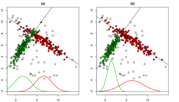
Figure 4: Simdata4: (a) Results for $c_{X}=1$, that forces equal scatters in the marginal distribution (the plotted densities, in the lower part of the figure, represent the normal fitted components); (b) Results for $c_{X}=20$, that allows different scatters. In both cases, $\alpha=0.1$ and $c_{\varepsilon}=20$ have been chosen.

On the other hand, the constant $c_{\varepsilon}$ represents the maximum ratio among the variances of the regression error terms. Even if the ML estimation would be attracted by solutions in which some $\sigma_{g}^{2}\rightarrow 0$, due to their high contribution by means of $\phi(y_{i};\mathbf{b}^{\prime}_{g}\mathbf{x}_{i}+b_{g}^{0},\sigma_{g}^{2})$ to the maximization of the log-likelihood in (4), a choice of $c_{\varepsilon}<\infty$ avoids that the algorithm fall into singularities. Enforcing a value $c_{\varepsilon}=1$ imposes the strongest constraint $\sigma_{1}^{2}=...=\sigma_{G}^{2}$. For instance, let us consider Simdata5 in Figure 5, which has been generated from a CWM with $\sigma_{1}^{2}=0.5^{2}$ and $\sigma_{2}^{2}=0.1^{2}$ ($\sigma_{1}^{2}/\sigma_{2}^{2}=25$). The results of fitting the trimmed CWRM for this data set are also shown with bands. Indeed, in specific applications, it is useful to take into account such bands, centered at the fitted regression lines and with amplitudes given by $\pm 2\sigma_{g}$, i.e. twice the estimated standard deviations of the regression error terms. A first solution corresponding to $c_{\varepsilon}=1<25$ is given in Figure 5 (a), while a second one corresponding to $c_{\varepsilon}=50>25$ is given in panel 5(b). Notice the different amplitude of these bands. However, although different scatters can be effective in many cases, a huge difference between them is not recommended, as it can lead to fit a few almost collinear observations.

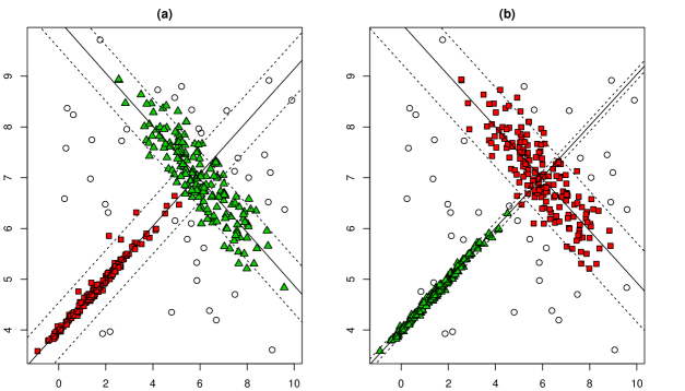
Figure 5: Simdata5: (a) Results for $c_{\varepsilon}=1$, forcing equal variances in the error terms. (b) Results for a larger $c_{\varepsilon}=20$ value. In both cases, $\alpha=0.1$ and $c_{X}=20$ have been chosen and bands of amplitude $\pm 2\sigma_{g}$ are shown.

An important feature of the proposed methodology is to provide a different constraint for the eigenvalues of the matrices $\mbox{\boldmath$\Sigma$}_{g}$ and for the variances of the error terms $\sigma_{g}^{2}$. This allows to deal with different scales in the explanatory and response variables, which is common in many applications. On the other hand, the procedure is not fully affine equivariant in the explanatory variables, due to the considered constraints. However, if needed, it is close to affine equivariance for large values of $c_{X}$.

It is well known, see e.g. Ingrassia et al. (2012), that the linear Gaussian CWM may be seen as included in the finite mixture of Gaussian distributions when embedding it into a $d+1$ dimensional space. Also in the latter case, constraints are needed to avoid singularities and to reduce the detection of spurious solutions. However, constraints giving a completely symmetric handling of the variability for the explanatory variables and for the error terms are not always the best idea. For instance, as a way to provide robustness, we could have considered the TCLUST methodology (García-Escudero et al., 2008) in the $d+1$ dimensional space which needs the specification of a constant $c\geq 1$ to constraint the maximal ratio among the $G\times(d+1)$ eigenvalues. Unfortunately, Mixture of Regressions problems often require very high values for the constant $c$ which do not always guarantee TCLUST to be correctly protected against spurious solutions.

To illustrate the previous claims, let us consider Simdata6, of size $n=200$, where 180 observations have been generated from a CWM with two groups, and 20 observation have been included as concentrated noise. The data set is plotted in Figure 6, where panel (a) shows the results of applying the TCLUST methodology with $c=1.5$ in dimension $d+1=2$. We can see that the results are not satisfactory (the analogous of the regression lines are the axes corresponding to the largest eigenvalue of the $\mbox{\boldmath$\Sigma$}_{g}$ matrices) and, therefore, higher $c$ values seem to be needed. But, higher $c$ values often yield the detection of undesired spurious solutions. For instance, panel (b) shows the results of applying TCLUST with $c=500$ with the detection of a cluster only containing all noisy observations. On the other hand, we can see that a proper fit is obtained in panel (c), when applying the trimmed CWRM with $c_{X}=c_{\varepsilon}=1.5$.

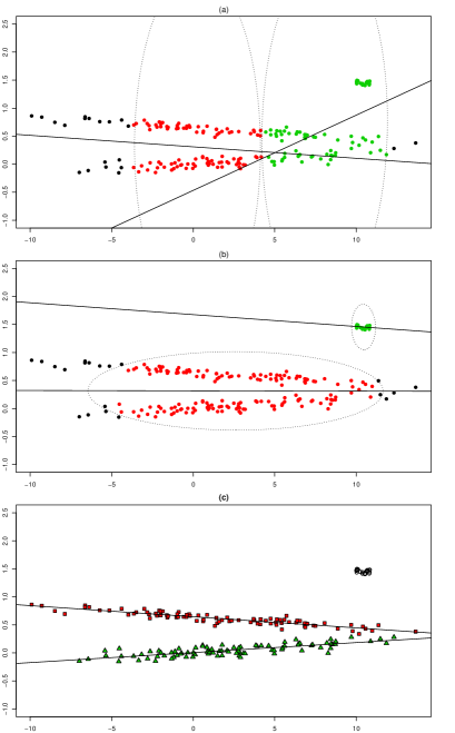
Figure 6: Simdata6: (a) TCLUST results with $c=1.5$ and $\alpha=0.1$; (b) TCLUST results with $c=500$ and $\alpha=0.1$; (c) Trimmed CWRM fitting results with $c_{X}=c_{\varepsilon}=1.5$ and $\alpha=0.1$.

It is worthy to note that asymmetric constraints also underlies some parameterizations already proposed in closely related problems as, for instance, in Dasgupta and Raftery (1998) where the eigenvalues of the scatter matrices corresponding to the $(d+1)$-dimensional fitted mixture components are requested to be $\lambda_{g}\times\{1,\alpha,...,\alpha\}$ with $\alpha<<1$.

4.2 Effect of trimming

We start from the well-known Mixture of Regressions model and first consider an easier trimming approach based on the maximization of

$$\sum_{i=1}^{n}z(\mathbf{x}_{i},y_{i})\log\left[\sum_{g=1}^{G}\phi(y_{i};\mathbf{b}^{\prime}_{g}\mathbf{x}_{i}+b_{g}^{0},\sigma_{g}^{2})\pi_{g}\right],$$ (10)

with $\sum_{i=1}^{n}z(\mathbf{x}_{i},y_{i})=[n(1-\alpha)]$ and imposing a constraint on the variances of the error terms $\sigma_{g_{1}}^{2}/\sigma_{g_{2}}^{2}\leq c_{\varepsilon}$ for $1\leq g_{1},g_{2}\leq G$. Notice that, in this case, the distribution of $\mathbf{X}$ is not taken into account, hence no trimming related to the $\mathbf{X}$ model is considered. This straightforward robust extension will be referred to as trimmed Mixture of Regressions (Neykov et al., 2007; García-Escudero et al., 2010). Apart from the constraints, this approach reduces to the traditional Mixture of Regressions when $\alpha=0$, and leads back to the widely-applied Least Trimmed Squares (LTS) method (see, e.g., Rousseeuw and Leroy, 1987) when $G=1$ and $\alpha>0$. It protects against large values of $(y_{i}-\mathbf{b}^{\prime}_{g}\mathbf{x}_{i}-b_{g}^{0})^{2}$, hence it is useful to cope with many cases of data contamination which cause the parameters $\mathbf{b}_{g}$ “breakdown”, in absence of trimming. However, it does not prevent the model estimation from the effects of “bad” leverage points, due to outliers in $\mathbf{x}$. As it happens in ordinary least squares regression, a few bad leverage points could provoke very disappointing results.

For instance, consider the simulated datasets Simdata7 and Simdata8 in Figure 7. Both datasets are made of 180 observations drawn from a CWM with two groups and with 20 noisy observations generated by two different contamination mechanisms. The leftmost panels in Figure 7,(a) and (d) show the results of fitting the standard CWM; the central panels (b) and (e) concern trimmed Mixture of Regressions ($\alpha=0.1$) and, finally, the rightmost panels (c) and (f) illustrate the proposed trimmed CWRM ($\alpha=0.1$). We can see that the fit of the standard (untrimmed) CWM is strongly affected by the contamination. Trimmed Mixtures of Regression are able to resist the type of contamination in (b) but cannot afford outliers acting as bad leverage points, as in (e). On the other hand, the use of trimmed CWRM, as shown in (c) and (f), resists both types of contamination. To avoid an unfair comparison, we have not included remarkable differences in the $\mathbf{X}$ distributions for the two main groups (i.e., prior to contamination), but we can see in Figure 1 how the trimmed CWRM is able to deal with components having different marginal distributions.

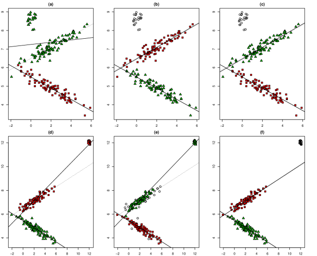
Figure 7: Simdata7 in the upper panels (a)-(c) and Simdata8 in the lower panels (d)-(f). (a) and (d) fitting the (untrimmed) CWM; (b) and (e) fitting trimmed Mixture of Regressions; (c) and (f) applying trimmed CWRM including a $10\%$ of contamination. In particular, $\alpha=0.1$ and $c_{\varepsilon}=20$ are used in (b), (c), (e) and (f), while $c_{X}=20$ is used in (c) and (f).

The problem of leverage points has been addressed in Robust Regression by down-weighting influential observations as, for instance, GM-estimators do (Krasker and Welsch, 1992). In the context of clusterwise regression, García-Escudero et al. (2010) proposed a “second trimming”, by fixing two trimming parameters $\alpha_{1}$ and $\alpha_{2}$. Parameter $\alpha_{1}$ controls the effect of outliers corresponding to large values of $(y_{i}-\mathbf{b}^{\prime}_{g}\mathbf{x}_{i}-b_{g}^{0})^{2}$ while $\alpha_{2}$ aims at controlling leverage points corresponding to outlying values on $\mathbf{x}$. However, the distinction between these two types of outliers is not always so clear. On the other hand, the unified handling of outliers provided by the trimmed CWRM simultaneously deals with both types of outliers. As the probability to belong to a cluster is not a fixed value, $\pi_{g}$, but depends also on the CWM weight $\phi_{d}(x_{i},\mbox{\boldmath$\mu$}_{g},\mbox{\boldmath$\Sigma$}_{g})\pi_{g}$, trimming acts before on points that lay on the farer contours of equiprobability (i.e. sets of points where the p.d.f. of the mixture takes a constant value) from the cluster means. We are assuming that outliers are the points $(\mathbf{x}_{i},y_{i})$ with lower values of $D(\mathbf{x}_{i},y_{i};\mbox{\boldmath$\theta$})$, rather than points with greater vertical distances $(y_{i}-\mathbf{b}^{\prime}_{g}\mathbf{x}_{i}-b_{g}^{0})^{2}$.

Other alternatives to guard CWM against contamination are based on the consideration of $t$-distributions, instead of normal ones, see Ingrassia et al. (2012). They provide a clear robustness gain with respect to the Gaussian CWM. However, without trimming, one single observation placed in a very remote position can still be very harmful. In fact, we can make some components of $\mathbf{b}_{g}$ to be arbitrarily large or small, just by moving one single observation. A small positive fraction of pointwise contamination can be very dangerous too, even when it is not distant from the data. On the other hand, the trimmed CWRM is more resistant to extreme contaminations, because it does not make any assumption about how outliers have been generated. Therefore, rather structured sources of outliers (and clearly not generated from a $t$-distribution) can be handled, too.

Several methods can be also found in the literature aimed at robustifying the Mixtures of Regressions model. Apart from those based on trimming that have been previously cited, methods based on M-estimation have been proposed in Bai et al. (2012) and extending S-estimation in Bashir and Carter (2012). Song et al. (2014) propose to model the error terms by a Laplace distribution, while Yao et al. (2014) suggest to employ the $t$ distribution. Although all these methods improve the robustness of the model, they do not model the marginal $\mathbf{X}$ distribution. Therefore, they do not take advantage of this information to detect the different mixture components and hence are not able to cope with outliers both on $\mathbf{x}$ and on $y$, acting as bad leverage points. To overcome this issue, Yao et al. (2014) have recently proposed applying their robust Mixture of Regression after using a trimming procedure (with high breakdown point) which removes clear outliers on $\mathbf{x}$. This initial trimming is unfortunately done without considering the $Y$ variable, nor the joint distribution in $(\mathbf{X},Y)$, corresponding to the different mixture components. The MCD estimator, considered for this initial trimming, is aimed at working on a single contaminated population and can be troublesome for detecting outliers when the data set includes different subpopulations.

In most of the applications, the true contamination level is unknown. Therefore, it makes sense to consider a preventive (higher than needed) trimming level $\alpha$. This could lead to wrongly trimmed observations, but the “cores” of the clusters and sensible approximations of the regression lines are most of the times correctly found. Starting from them, it is not difficult to recover wrongly trimmed observations, by resorting to Mahalanobis distances and diagnostic regression tools (see Section 7 in García-Escudero et al., 2010).

5 Real data examples

5.1 Tone data

This data set comes from an experiment in music perception introduced in Cohen (1984) which has been analyzed in many papers concerning Mixtures of Regression, (see, e.g. de Veaux, 1989) and their robust versions (Schlittgen, 2011; Hennig, 2002; Bai et al., 2012; Bashir and Carter, 2012; Song et al., 2014; Yao et al., 2014). This data set is shown in Figure 8(a) and the result of applying the trimmed CWRM in (b). We can see that the two main groups (interval memory judgement and partial matching) can be detected by applying the trimmed CWRM. Furthermore, $\alpha=0.05$ allows to detect a fraction of outlying observations, within the partial matching group, exhibiting a clear different behavior.

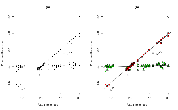
Figure 8: Tone data: (a) Data set; (b) Trimmed CWRM fitting with $\alpha=0.05$ and $c_{X}=c_{\varepsilon}=20$.

The type of outliers included in this data set are not very harmful and, thus, no dramatic differences can be expected in terms of the estimated parameters, when using any (robust) Mixture of Regressions approach. So, we will proceed to artificially contaminate the data and use it as a benchmark for the effects of leverage points added through pointwise contamination. This has been already done by Bai et al. (2012), who introduced a $6\%$ of contamination at $(0,4)$, when applying an M-estimation approach. In our case, we will use a more complete contamination scheme by adding $9\%$ of point contamination, placed around points $(2.5,5)$, $(6,4)$, $(0,0.5)$ and $(5,2.5)$, successively. The first location, $(2.5,5)$ is a regression outlier, while the remaining three are leverage points.

Contamination		Trimmed CWRM	Discarded		Trimmed MR	Discarded
location		constants	outliers		constants	outliers
$(2.5,5)$		$c_{X}=c_{\varepsilon}=1$	Yes		$c_{\varepsilon}=1$	Yes
		$c_{X}=c_{\varepsilon}=10^{3}$	No		$c_{\varepsilon}=10^{3}$	Yes
		$c_{X}=c_{\varepsilon}=10^{10}$	No		$c_{\varepsilon}=10^{10}$	No
$(6,4)$		$c_{X}=c_{\varepsilon}=1$	Yes		$c_{\varepsilon}=1$	No
		$c_{X}=c_{\varepsilon}=10^{3}$	No		$c_{\varepsilon}=10^{3}$	No
		$c_{X}=c_{\varepsilon}=10^{10}$	No		$c_{\varepsilon}=10^{10}$	No
$(0,0.5)$		$c_{X}=c_{\varepsilon}=1$	Yes		$c_{\varepsilon}=1$	No
		$c_{X}=c_{\varepsilon}=10^{3}$	Yes		$c_{\varepsilon}=10^{3}$	No
		$c_{X}=c_{\varepsilon}=10^{10}$	No		$c_{\varepsilon}=10^{10}$	No
$(5,2.5)$		$c_{X}=c_{\varepsilon}=1$	Yes		$c_{\varepsilon}=1$	No
		$c_{X}=c_{\varepsilon}=10^{3}$	No		$c_{\varepsilon}=10^{3}$	No
		$c_{X}=c_{\varepsilon}=10^{10}$	No		$c_{\varepsilon}=10^{10}$	No

Table 1: Tone data: Performance comparison between the trimmed CWRM methodology and trimmed Mixture of Regressions (trimmed MR) with an $\alpha=0.1$ trimming level.

Table 1 summarizes the performance of the proposed trimmed CWRM and the trimmed Mixture of Regressions (trimmed MR) presented in Section 4.2, both with an $\alpha=0.1$ trimming level, for different values of the constraints factors $c_{X}$ and $c_{\varepsilon}$, and labeling by “Yes”/“No” the cases in which the trimming level allows/does not allow to discard all the noisy observations. We can see that only the use of the trimmed CWRM with $\alpha=0.1$ and with both constants fixed at their most restrictive values is able to cope with the contamination in all the considered scenarios.

5.2 Students’ heights and weights

The data set in this example is based on students answers to a questionnaire including simple questions about anthropometric measurements. Due to the way in which the dataset has been collected, it contains outliers, as some students did not seriously answer the questions, or gave bad interpretations of the measurement units, etc. Here, we focus on the relationship between two variables in the data set, namely “Height” ($X$) in cm and “Weight” ($Y$) in Kg. Although gender was also considered in the study, we will ignore it, to test the ability of our methodology to classify the individuals and to estimate the two underlying regression models, one for each gender, in presence of an important amount of severe outliers.

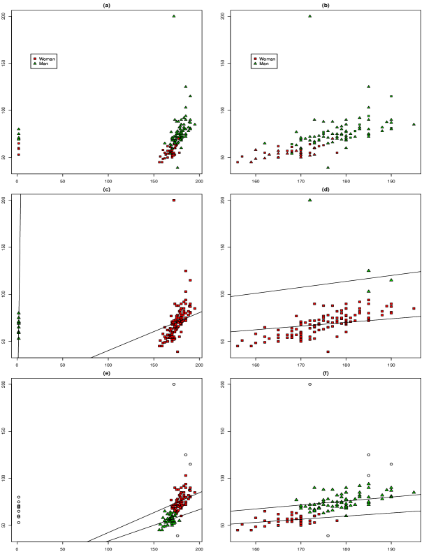
Figure 9: Student data: (a) “Students’ heights and weights” data. (b) Cleaned data set obtained by deleting the outliers due to wrong measurement scale for “height”. Effects of trimming and restrictions on CRWM results: (c) untrimmed and almost unrestricted: $\alpha=0$ and $c_{X}=c_{\varepsilon}=10^{10}$; (d) untrimmed and almost unrestricted: $\alpha=0$ and $c_{X}=c_{\varepsilon}=10^{10}$ for the cleaned data set; (e) trimmed and constrained: $\alpha=0.1$ and $c_{X}=c_{\varepsilon}=20$; (f) trimmed and constrained: $\alpha=0.04$ and $c_{X}=c_{\varepsilon}=20$ for the cleaned data set

Figure 9(a) shows the original data set (which will be referred to as Student data) with the true gender assignments, while in (b) we have eliminated the points corresponding to a wrong scale in height (students reporting height in meters instead of centimeters), to emphasize the different linear patterns. Several implausible weight values can be also seen. Figure 9(c) shows the results corresponding to the fit of the CWM (when $\alpha=0$ and $c_{x}=c_{\epsilon}=10^{10}$, i.e., no trimming and almost unrestricted). We can see that one of the regression lines is capturing the artificial group, almost collinear, having anomalous height values. Consequently, the main groups are joined together and the classification error rate is very high. On the other hand, Figure 9(e) shows the result of applying the trimmed CWRM with $\alpha=0.1$ and moderate values of the constraints. Restrictions now avoid that the method falls into the previously obtained spurious solution, generated by the almost collinear outliers (wrong measurement units) and these points are trimmed off, together with other data points exhibiting atypical weight values. The classification error rate for untrimmed observations is just $12\%$. Figures 9(d) and (f) show the data set after eliminating the points with wrong units for the height. In Figure 9(d), we can see that using the CWM, even in this cleaned data set, again fails to detect the true groups. On the contrary, we can see in (f) that the trimmed CWRM with $\alpha=0.04$ and moderate values of $c_{X}$ and $c_{\epsilon}$ provides sensible results. It is true that simple visual inspection could have served to “clean” this data set but this is surely not the case when dealing with more complex/high dimensional data sets on when carrying out fully unsupervised data analyses.

6 Concluding remarks

The present work is centered on the wide family of Gaussian CWMs, that received a growing attention in the recent literature. However, like it happens for many other models which depend on normal assumptions, the ML estimation for CWM suffers from a lack of robustness. Moreover, the problem statement in terms of the likelihood maximization is not well-posed, without constraints. Hence, here we have presented a new estimation framework for the linear Gaussian CWM based on trimming and constraints, to achieve robustness, identify and discard outliers, circumvent the likelihood singularities and reduce the detection of spurious solutions.

Numerical studies, based on both simulated and real data, show that the new proposal drives the estimation procedure to discard even strongly concentrated contaminating observations, acting as bad leverage points, which are so harmful in the framework of Mixtures of Regressions. Apart from the effectiveness of the proposed methodology to resist to any kind of outliers, we have also shown that a theoretically well defined mathematical and statistical problem underlies it. The existence of optima for both the population and the sample problem have been established, and the consistency of the sample solution to the population one has been provided.

Further research could be focused on tuning the choice of the involved parameters. This is a complex task, as these parameters are clearly interrelated. For instance, a high trimming level $\alpha$ could lead to smaller $G$ values, since components with fewer observations may be trimmed off. Moreover, larger values of $c_{X}$ and $c_{\varepsilon}$ could lead to higher values of $G$, since more components with few observations, but close to collinearity, may be detected. Our suggestion is that the researcher must provide in advance part of these parameters (as a way of specifying the type of clusters expected from the data) and, then, some data-dependent diagnostic can be used to make appropriate choices for the rest of parameters. The use of trimmed BIC notions (Neykov et al., 2007) or the adaptation of some graphical tools, as in García-Escudero et al. (2011), can be useful for this purpose.

Appendix

The following section is organized into four parts: part A contains technical lemmas useful for the proof of the existence of the maximizer $\theta$ for $L(\mbox{\boldmath$\theta$},P)$ (Proposition 3.2.1) which is established in part B; part C shows preliminary results needed to show the consistency of $\hat{\mbox{\boldmath$\theta$}}$ as an estimator for $\theta$ (Proposition 3.2.2), which is then proved in part D.

Part A: Preliminary results in view of Proposition 3.2.1

Four technical lemmas will be needed before attacking the proof of Proposition 3.2.1.

First of all, let us remark that, given the definition of $L(\mbox{\boldmath$\theta$},P)$, there exist sequences $\{\mbox{\boldmath$\theta$}_{n}\}_{n=1}^{\infty}$ with

$$\mbox{\boldmath$\theta$}_{n}=(\pi_{1}^{n},...,\pi_{G}^{n},\allowbreak\mbox{\boldmath$\mu$}_{1}^{n},...,\mbox{\boldmath$\mu$}_{G}^{n},\mbox{\boldmath$\Sigma$}_{1}^{n},...,\mbox{\boldmath$\Sigma$}_{G}^{n},b_{1}^{0,n},...,b_{G}^{0,n},\mathbf{b}_{1}^{n},...,\mathbf{b}_{G}^{n},\allowbreak\sigma_{1}^{2,n},...,\sigma_{G}^{2,n}),$$ (11)

and $\mbox{\boldmath$\theta$}_{n}\in\Theta_{c_{X},c_{\varepsilon}}$ and such that

$$\lim_{n\rightarrow\infty}L(\mbox{\boldmath$\theta$}_{n},P)=\sup_{\mbox{\boldmath$\theta$}\in\Theta_{c_{X},c_{\varepsilon}}}L(\mbox{\boldmath$\theta$},P)>-\infty$$ (12)

(the boundedness from below is obtained just by considering the set $A$ as being a ball centered at $(\mathbf{0},0)$ with $P[A]\geq 1-\alpha$, $\pi_{1}=1$, $\mbox{\boldmath$\mu$}_{1}=\mathbf{0}$, $\mbox{\boldmath$\Sigma$}_{1}=I_{d}$, $b_{1}^{0}=0$ and $\mathbf{b}_{1}=\mathbf{0}$).

The proof of the existence will be done by proving that we can obtain a convergent subsequence extracted from $\{\mbox{\boldmath$\theta$}_{n}\}_{n=1}^{\infty}$ satisfying (12), and whose limit $\mbox{\boldmath$\theta$}_{0}$ is optimal for $P$.

Let us begin with Lemma 1, which provides a uniformly bounded representation of the regression coefficients, even in case of local collinearity, without loosing their properties in the evaluation of the target function.

Lemma 1

Let $\{b_{n}^{0}\}_{n=1}^{\infty}$ be a sequence in $\mathbb{R}$, $\{\mathbf{b}_{n}\}_{n=1}^{\infty}$ be a sequence in $\mathbb{R}^{d}$ and $\{A_{n}\}_{n=1}^{\infty}$ be a sequence of sets in $\mathbb{R}^{d+1}$ verifying

$$\lim\sup_{n}P[A_{n}]>0$$ (13)

and such that

$$\lim\sup_{n}E_{P}\big{[}|b_{n}^{0}+\mathbf{b}_{n}^{\prime}\mathbf{X}-Y|^{2}I_{A_{n}}(\mathbf{X},Y)\big{]}<\infty.$$ (14)

Then, we can extract subsequences $\{b_{n_{k}}^{0}\}_{k=1}^{\infty}$, $\{\mathbf{b}_{n_{k}}\}_{k=1}^{\infty}$ and $\{A_{n_{k}}\}_{k=1}^{\infty}$ from them and define new sequences $\{d_{k}^{0}\}_{k=1}^{\infty}$, $\{\mathbf{d}_{k}\}_{k=1}^{\infty}$ and $\{D_{k}\}_{k=1}^{\infty}$ which satisfy $D_{k}\subseteq A_{n_{k}}$, $P[A_{n_{k}}\setminus D_{k}]\rightarrow 0$, $d_{n_{k}}^{0}\rightarrow d^{0}\in\mathbb{R}$, $\mathbf{d}_{n_{k}}\rightarrow\mathbf{d}\in\mathbb{R}^{d}$ and such that

$$(b_{n_{k}}^{0}+\mathbf{b}_{n_{k}}^{\prime}\mathbf{X}-Y)I_{D_{k}}(\mathbf{X},Y)=(d_{k}^{0}+\mathbf{d}_{k}^{\prime}\mathbf{X}-Y)I_{D_{k}}(\mathbf{X},Y),\text{ }P\text{-a.s.},$$ (15)

for every $k\geq 1$.

Proof: To simplify the proof, w.l.o.g., we will use the same notation for the subsequences as that used for the original sequences. If the sequences $\{b_{n}^{0}\}_{n=1}^{\infty}$ and $\{\mathbf{b}_{n}\}_{n=1}^{\infty}$ are bounded, then we just need to extract convergent subsequences and set $D_{n}=A_{n}$. So, let us assume that either one or both sequences are unbounded, and consider a sequence of compact sets $\{K_{n}\}_{n=1}^{\infty}$ such that $K_{n}\uparrow\mathbb{R}^{d+1}$. Let $\{\mathbf{v}_{n_{l}}\}_{l=1}^{d}$ be the normalized eigenvectors obtained from the spectral decomposition of the matrices $\{\text{Var}_{P}[\mathbf{X}/A_{n}\cap K_{n}]\}_{n=1}^{\infty}$ (we use $E_{P}[\cdot/A]$ and $\text{Var}_{P}[\cdot/A]$ for denoting $E_{P}[\cdot/(\mathbf{X},Y)\in A]$ and $\text{Var}_{P}[\cdot/(\mathbf{X},Y)\in A]$).

Now, let us suppose that there exists a direction $\mathbf{v}_{n_{l}}$ such that $\text{Var}_{P}[\mathbf{v}_{n_{l}}^{\prime}\mathbf{X}/A_{n}\cap K_{n}]\rightarrow 0$ then take $H$ with $0\leq H<d$ and such that $\text{Var}_{P}[\mathbf{v}_{n_{l}}^{\prime}\mathbf{X}/A_{n}\cap K_{n}]\rightarrow 0$ for every $l\geq H+1$, after a possible reordering of the coordinates. In this case, there also exist points $\{\mathbf{u}_{n_{l}}\}_{l=H+1}^{d}$ in $\mathbb{R}^{d}$ and a sequence $\varepsilon_{n}\downarrow 0$ which must satisfy $E_{P}[|\mathbf{v}_{n_{l}}^{\prime}(\mathbf{X}-\mathbf{u}_{n_{l}})|>\varepsilon_{n}/A_{n}\cap K_{n}]\rightarrow 0$ for every $l\geq H+1$. The $\mathbf{v}_{n_{l}}$ are bounded (unitary vectors) and the $\mathbf{u}_{n_{l}}$ must be bounded too (because, otherwise, $\mathbf{X}$ would not be tight). Therefore, there exist subsequences, that will be denoted as the original ones, such that $\mathbf{v}_{n_{l}}\rightarrow\mathbf{v}_{l}\in\mathbb{R}^{d}$, $\mathbf{u}_{n_{l}}\rightarrow\mathbf{u}_{l}\in\mathbb{R}^{d}$ and $P[|\mathbf{v}_{l}^{\prime}(\mathbf{X}-\mathbf{u}_{l})|>0/A_{n}\cap K_{n}]\rightarrow 0$ for every $l\geq H+1$.

Let us now define $D_{n}=A_{n}\cap K_{n}\cap_{l=H+1}^{d}\{\mathbf{v}_{l}^{\prime}(\mathbf{X}-\mathbf{u}_{l})=0\}$ which trivially verifies $D_{n}\subset A_{n}$ and that $P[A_{n}\setminus D_{n}]\rightarrow 0$. We can rewrite

$$b_{n}^{0}+\mathbf{b}_{n}^{\prime}\mathbf{x}=b_{n}^{0}+\sum_{l=1}^{H}\mathbf{b}_{n}^{\prime}\mathbf{v}_{l}\mathbf{v}_{l}^{\prime}\mathbf{x}+\sum_{l=H+1}^{d}\mathbf{b}_{n}^{\prime}\mathbf{v}_{l}\mathbf{v}_{l}^{\prime}\mathbf{x}.$$

and set $d_{n}^{0}=b_{n}^{0}+\sum_{l=H+1}^{d}\mathbf{b}_{n}^{\prime}\mathbf{u}_{l}$ and $\mathbf{d}_{n}=\sum_{l=1}^{H}\mathbf{b}_{n}^{\prime}\mathbf{v}_{l}\mathbf{v}_{l}^{\prime}$ for $H>0$ (while we set $\mathbf{d}_{n}=\mathbf{0}$ when $H=0$). Then (15) trivially holds and it can be shown that $\{d_{n}^{0}\}_{n=1}^{\infty}$ and $\{\mathbf{d}_{n}\}_{n=1}^{\infty}$ are bounded sequences. This follows from the fact that (14) guarantees that $\{(b_{n}^{0}+\mathbf{b}_{n}^{\prime}\mathbf{X}-Y)I_{D_{n}}(\mathbf{X},Y)\}_{n=1}^{\infty}$ is a tight sequence. Notice that we could see that the previous tightness property would be contradicted if any of the $\{d_{n}^{0}\}_{n=1}^{\infty}$ and $\{\mathbf{d}_{n}\}_{n=1}^{\infty}$ were unbounded by seeing that $\mathbf{Z}=(Z_{1},...,Z_{H})$ with $Z_{l}=\mathbf{v}_{l}^{\prime}\mathbf{x}$ satisfies $\det(\text{Var}_{P}[\mathbf{Z}/A_{n}\cap K_{n}])>0$ and $\mathbf{d}_{n}^{\prime}\mathbf{x}=\sum_{l=1}^{H}\mathbf{b}_{n}^{\prime}\mathbf{v}_{l}Z_{l}$.

Finally, whenever none of the sequences $\text{Var}_{P}[\mathbf{v}_{n_{l}}^{\prime}\mathbf{X}/A_{n}\cap K_{n}]$ converges to 0, we can consider the representation $b_{n}^{0}+\mathbf{b}_{n}^{\prime}\mathbf{x}=b_{n}^{0}+\sum_{l=1}^{H}\mathbf{b}_{n}^{\prime}\mathbf{v}_{l}\mathbf{v}_{l}^{\prime}\mathbf{x}$ and the result would be proven in this case, too, following similar arguments as before. $\Box$

The following Lemma 2 assures that, under the usual assumption on $P$, the associated fitted trimmed CWMs could not be arbitrarily close to a degenerated model concentrated on $G$ points, nor on $G$ regression hyperplanes.

Lemma 2

Let $P$ be a distribution in $\mathbb{R}^{d+1}$ satisfiying (PR):

1. For every $b_{g}^{0}\in\mathbb{R}$, $\mathbf{b}_{g}\in\mathbb{R}^{d}$ and $A\subseteq\mathbb{R}^{d+1}$ with $P[A]=1-\alpha$, there exists $\delta>0$ such that

   $$E_{P}\bigg{[}\min_{g=1,...,G}|b_{g}^{0}+\mathbf{b}_{g}^{\prime}\mathbf{X}-Y|^{2}I_{A}(\mathbf{X},Y)\bigg{]}\geq\delta.$$

2. For every set of $G$ points $\{\mathbf{\mbox{\boldmath$\mu$}}_{1},...,\mathbf{\mbox{\boldmath$\mu$}}_{G}\}\subset\mathbb{R}^{d}$ and $A\subseteq\mathbb{R}^{d+1}$ with $P[A]=1-\alpha$, there exists $\delta>0$ such that

   $$E_{P}\bigg{[}\min_{g=1,...,G}\|\mathbf{X}-\mathbf{\mbox{\boldmath$\mu$}}_{g}\|^{2}I_{A}(\mathbf{X},Y)\bigg{]}\geq\delta.$$

Proof of (a): Let us suppose that $\delta$ does not exist. Then, we can choose sequences $\{A_{n}\}_{n=1}^{\infty}$, $\{b_{g}^{0,n}\}_{n=1}^{\infty}$ and $\{\mathbf{b}_{g}^{n}\}_{n=1}^{\infty}$ such that

$$E_{P}\bigg{[}\min_{g=1,...,G}|b_{g}^{0,n}+(\mathbf{b}_{g}^{n})^{\prime}\mathbf{x}-y|^{2}I_{A_{n}}(\mathbf{x},y)\bigg{]}\rightarrow 0\text{ with }P[A_{n}]\rightarrow 1-\alpha.$$ (16)

Moreover, we can replace the sets $A_{n}$ in (16), by the data sets

$$A_{n}^{*}=\big{\{}(\mathbf{x},y):\min_{g=1,...,G}|b_{g}^{0,n}+(\mathbf{b}_{g}^{n})^{\prime}\mathbf{x}-y|^{2}\leq\min\{r_{\alpha}^{n},\varepsilon\}\big{\}},$$

where $r_{\alpha}^{n}=\inf_{u}\{P[(\mathbf{x},y):\min_{g=1,...,G}\allowbreak|b_{g}^{0,n}+(\mathbf{b}_{g}^{n})^{\prime}\mathbf{x}-y|^{2}\leq u]\geq 1-\alpha\}$ and we also have the same convergence as in (16), with $P[A_{n}^{*}]\rightarrow 1-\alpha$ for any fixed choice of $\varepsilon>0$. Then, take

$$A_{g}^{n}=\bigg{\{}(\mathbf{x},y)\in A_{n}^{*}:|b_{g}^{0,n}+(\mathbf{b}_{g}^{n})^{\prime}\mathbf{x}-y|=\min_{j=1,...,G}|b_{j}^{0,n}+(\mathbf{b}_{j}^{n})^{\prime}\mathbf{x}-y|\bigg{\}},$$

and, we can see that there exists at least one $g$ such that $P[A_{g}^{n}]\rightarrow p_{g}>0$ through a subsequence (because $P[A_{n}^{*}]=\sum_{g=1,...,G}P[A_{g}^{n}]\rightarrow 1-\alpha$). Thus, consider a reordering of $\{1,...,G\}$ such that $P[A_{g}^{n}]\rightarrow p_{g}>0$ for every $g\in\{1,...,H\}$ (for an appropriate subsequence, if needed). If $A_{n}^{**}=\cup_{g=1}^{H}A_{g}^{n}$, then

$$E_{P}\bigg{[}\min_{g=1,...,G}|b_{g}^{0,n}+(\mathbf{b}_{g}^{n})^{\prime}\mathbf{X}-Y|^{2}I_{A_{n}^{**}}(\mathbf{X},Y)\bigg{]}$$

$$\quad\quad\quad\quad\quad\quad=\sum_{g=1}^{H}E_{P}\bigg{[}|b_{g}^{0,n}+(\mathbf{b}_{g}^{n})^{\prime}\mathbf{X}-Y|^{2}I_{A^{n}_{g}}(\mathbf{X},Y)\bigg{]}$$

and $P[A_{n}^{**}]\rightarrow 1-\alpha$. For every $g\in\{1,...,H\}$, the $A_{g}^{n}$, $b_{g}^{0,n}$ and $\mathbf{b}_{g}^{n}$ satisfy the conditions needed to apply Lemma 1 and, therefore, we can replace them by $D_{g}^{n}$, $d_{g}^{0,n}$ and $\mathbf{d}_{g}^{n}$ satisfying $D_{g}^{n}\subset A_{g}^{n}$, $P[A_{g}^{n}\setminus D_{g}^{n}]\rightarrow 0$, $d_{g}^{0,n}\rightarrow d_{g}^{0}\in\mathbb{R}$ and $\mathbf{d}_{g}^{n}\rightarrow\mathbf{d}_{g}^{0}\in\mathbb{R}^{d}$ and (15).

Now, take $B_{n}=\cup_{g=1,...,H}D_{g}^{n}\cap\{(\mathbf{x},y):\min_{g=1,...,G}|d_{g}^{0,n}+(\mathbf{d}_{g}^{n})^{\prime}\mathbf{x}-y|^{2}\leq\varepsilon\}$ for a fixed $\varepsilon$, with $P[B_{n}]\rightarrow 1-\alpha$. We thus have the pointwise convergence

$$\min_{g=1,...,H}|d_{g}^{0,n}+(\mathbf{d}_{g}^{n})^{\prime}\mathbf{x}-y|^{2}I_{B_{n}}(\mathbf{x},y)\rightarrow\min_{g=1,...,H}|d_{g}^{0}+(\mathbf{d}_{g}^{0})^{\prime}\mathbf{x}-y|^{2}I_{B_{0}}(\mathbf{x},y),$$

for any $B_{0}\subset\mathbb{R}^{d+1}$ with $P[B_{0}]=1-\alpha$, and the uniform bound $\min_{g=1,...,H}|d_{g}^{0,n}+(\mathbf{d}_{g}^{n})^{\prime}\mathbf{X}-Y|^{2}I_{B_{n}}(\mathbf{x},y)\leq\varepsilon.$ Then, the dominated convergence theorem implies

$$E_{p}\bigg{[}\min_{g=1,...,H}|d_{g}^{0,n}+(\mathbf{d}_{g}^{n})^{\prime}\mathbf{X}-Y|^{2}I_{B_{n}}(\mathbf{X},Y)\bigg{]}$$

$$\quad\quad\quad\quad\quad\quad\rightarrow E_{p}\bigg{[}\min_{g=1,...,H}|d_{g}^{0}+(\mathbf{d}_{g}^{0})^{\prime}\mathbf{X}-Y|^{2}I_{B_{0}}(\mathbf{X},Y)\bigg{]}.$$

The latter convergence and (16) would prove that

$$E_{p}\bigg{[}\min_{g=1,...,H}|d_{g}^{0}+(\mathbf{d}_{g}^{0})^{\prime}\mathbf{X}-Y|^{2}I_{B_{0}}(\mathbf{X},Y)\bigg{]}=0,$$

implying that the distribution $P$ is concentrated on $G$ regression hyperplanes after removing a proportion $\alpha$ of the probability mass and this would contradict (PR).

Proof of (b): The proof of this results mimics the steps followed in the proof of (a). We start by assuming the existence of subsequences $\{A_{n}\}_{n=1}^{\infty}$ and $\{\mbox{\boldmath$\mu$}_{g}^{n}\}_{n=1}^{\infty}$ such that

$$E_{P}\bigg{[}\min_{g=1,...,G}\|\mathbf{x}-\mbox{\boldmath$\mu$}_{g}^{n}\|^{2}I_{A_{n}}(\mathbf{x},y)\bigg{]}\rightarrow 0\text{ with }P[A_{n}]\rightarrow 1-\alpha.$$

and we would end up by seeing that the support $\mathbf{X}$ is concentrated in $G$ points in $\mathbb{R}^{d}$. In fact, the proof is easier because only the tightness of $P$ is needed (Lemma 1 is no longer required, here). $\Box$

Now, since $[0,1]^{G}$ is a compact set, we can trivially choose a subsequence of $\{\mbox{\boldmath$\theta$}_{n}\}_{n=1}^{\infty}$ such that $\pi_{g}^{n}\rightarrow\pi_{g}\in[0,1]\text{ for }1\leq g\leq G.$ With respect to the scatter matrices and the variances of the error terms, we have the following possibilities:

$$\text{(S1) }\mbox{\boldmath$\Sigma$}_{g}^{n}\rightarrow\mbox{\boldmath$\Sigma$}_{g}\text{ for }1\leq g\leq G\text{ with }\mbox{\boldmath$\Sigma$}_{g}\text{ being p.s.d. matrices}$$

$$\text{(S2) }\min_{g=1,...,G}\min_{l=1,...,d}\lambda_{l}(\mbox{\boldmath$\Sigma$}_{g}^{n})\rightarrow\infty$$

$$\text{(S3) }\max_{g=1,...,G}\max_{l=1,...,d}\lambda_{l}(\mbox{\boldmath$\Sigma$}_{g}^{n})\rightarrow 0$$

$$\text{(V1) }\sigma_{g}^{2,n}\rightarrow\sigma_{g}^{2}\text{ for }1\leq g\leq G\text{ with }\sigma_{g}>0$$

$$\text{(V2) }\min_{g=1,...,G}\sigma_{g}^{2,n}\rightarrow\infty$$

$$\text{(V3) }\max_{g=1,...,G}\sigma_{g}^{2,n}\rightarrow 0$$

Given that $\mbox{\boldmath$\theta$}_{n}\in\Theta_{c_{X},c_{\varepsilon}}$, only one of the convergences in S1-S3 and only one in V1-V3 are possible, and the following Lemma 3 will further delimitate to the bounded results, based on constraints (5) and (6).

Lemma 3

If $\{\mbox{\boldmath$\theta$}_{n}\}_{n=1}^{\infty}\subset\Theta_{c_{X},c_{\varepsilon}}$ converges toward the supremum of $L(\mbox{\boldmath$\theta$},P)$, and (PR) holds for $P$, then only convergences (S1) and (V1) are possible.

Proof: We have that $L(\mbox{\boldmath$\theta$}_{n};P)$ can be bounded from above by

$$-\frac{1}{2}\left[\log\bigg{(}\min_{g}\sigma_{g}^{2,n}\bigg{)}P[A(\mbox{\boldmath$\theta$}_{n})]+\frac{E_{P}\big{[}\min_{g}|b_{g}^{0,n}+(\mathbf{b}_{g}^{n})^{\prime}\mathbf{X}-Y|^{2}I_{A(\mbox{\boldmath$\theta$}_{n})}(\mathbf{X},Y)\big{]}}{\max_{g}\sigma_{g}^{2,n}}\right]\\$$

$$\hskip 4.26773pt-\frac{1}{2}\left[\log\bigg{(}\min_{g}\min_{l}\lambda_{l}(\mbox{\boldmath$\Sigma$}_{g}^{n})\bigg{)}P[A(\mbox{\boldmath$\theta$}_{n})]d+\frac{E_{P}\big{[}\min_{g}\|\mathbf{X}-\mbox{\boldmath$\mu$}_{g}^{n}\|^{2}I_{A(\mbox{\boldmath$\theta$}_{n})}(\mathbf{X},Y)\big{]}}{\max_{g}\max_{l}\lambda_{l}(\mbox{\boldmath$\Sigma$}_{g}^{n})}\right]+C,$$

where $C$ is a constant value, not depending on $\mbox{\boldmath$\theta$}_{n}$.

Therefore, given that $\mbox{\boldmath$\theta$}_{n}\in\Theta_{c_{X},c_{\varepsilon}}$, we see that the possible convergence of $L(\mbox{\boldmath$\theta$}_{n};P)$ would clearly depend on those for the sequences

$$\log\bigg{(}\frac{\sigma_{n}^{2}}{c_{\varepsilon}}\bigg{)}P[A(\mbox{\boldmath$\theta$}_{n})]+E_{P}\bigg{[}\min_{g}\big{|}b_{g}^{0,n}+(\mathbf{b}_{g}^{n})^{\prime}\mathbf{X}-Y\big{|}^{2}I_{A(\mbox{\boldmath$\theta$}_{n})}(\mathbf{X},Y)\bigg{]}\frac{1}{\sigma_{n}^{2}}$$ (17)

and

$$\log\bigg{(}\frac{\lambda_{n}}{c_{X}}\bigg{)}P[A(\mbox{\boldmath$\theta$}_{n})]d+E_{P}\bigg{[}\min_{g}\|\mathbf{X}-\mbox{\boldmath$\mu$}_{g}^{n}\|^{2}I_{A(\mbox{\boldmath$\theta$}_{n})}(\mathbf{X},Y)\bigg{]}\frac{1}{\lambda_{n}},$$ (18)

where $\lambda_{n}=\max_{g=1,...,G}\max_{l=1,...,d}\lambda_{l}(\mbox{\boldmath$\Sigma$}_{g}^{n})$ and $\sigma_{n}^{2}=\max_{g=1,...,G}\sigma_{g}^{2,n}$.

On the other hand, Lemma 2 implies that a constant $\delta>0$ can be chosen such that $E_{P}\big{[}\min_{g}|b_{g}^{0,n}+(\mathbf{b}_{g}^{n})^{\prime}\mathbf{X}-Y|^{2}I_{A_{n}}(\mathbf{X},Y)\big{]}$ and $E_{P}\big{[}\min_{g}\|\mathbf{X}-\mbox{\boldmath$\mu$}_{g}\|^{2}I_{A_{n}}(\mathbf{X},Y)\big{]}$ in (17) and (18) are uniformly bounded from below by $\delta$. Therefore, other convergences different from (S1) or (V1) would imply that $\lim_{n\rightarrow\infty}L(\mbox{\boldmath$\theta$}_{n},P)=-\infty$ and this would contradict (12). $\Box$

Lemma 4, stated below, shows that we can always find a subsequence $\{\mbox{\boldmath$\theta$}_{n}\}_{n=1}^{\infty}$ with converging parameters for at least one mixture component, with weight $\pi_{g}^{n}$ converging toward a strictly positive value.

Lemma 4

There exists a sequence $\{\mbox{\boldmath$\theta$}_{n}\}_{n=1}^{\infty}$ converging toward the supremum of $L(\mbox{\boldmath$\theta$},P)$ and there exists $H$ with $1\leq H\leq G$ such that

$$\mbox{\boldmath$\mu$}_{g}^{n}\rightarrow\mbox{\boldmath$\mu$}_{g},\quad b_{g}^{0,n}\rightarrow b_{g}^{0},\quad\mathbf{b}_{g}^{n}\rightarrow\mathbf{b}_{g}\quad\textrm{and}\quad\pi_{g}^{n}\rightarrow\pi_{g}>0\quad\textrm{for every}\quad g\leq H$$

and such that the corresponding $\{A(\mbox{\boldmath$\theta$}_{n})\}_{n=1}^{\infty}$ sets are uniformly bounded.

Proof: Let us start from any $\{\mbox{\boldmath$\theta$}_{n}\}_{n=1}^{\infty}$ converging toward the supremum of $L(\mbox{\boldmath$\theta$},P)$, and take $A_{n}=A(\mbox{\boldmath$\theta$}_{n})$ and

$$A_{g}^{n}=\big{\{}(\mathbf{x},y)\in A_{n}:D_{g}(\mathbf{x},y;\mbox{\boldmath$\theta$})=\max_{j=1,...,G}D_{j}(\mathbf{x},y;\mbox{\boldmath$\theta$})\big{\}}$$

for $1\leq g\leq G$. Since $P[A_{g}^{n}]\in[0,1]$, there exists a subsequence, denoted as the original one, such that each $P[A_{g}^{n}]$ converges for $1\leq g\leq G$. Moreover, after a proper reordering in the components of $\mbox{\boldmath$\theta$}_{n}$, there exists $H^{*}\geq 1$ such that $P[A_{g}^{n}]\rightarrow p_{g}>0$ for $1\leq g\leq H^{*}$. Note that this $H^{*}$ does exist because otherwise we would have $P[A_{n}]=\sum_{g=1}^{G}P[A_{g}^{n}]\rightarrow 0$.

We can also find a convergent subsequence of $\mbox{\boldmath$\mu$}_{g}^{n}$ for every $g\leq H^{*}$. Otherwise, for every $\eta$ with $0<\eta<p_{g}$, we could take a ball $B_{g}$ centered at $(\mathbf{0},0)$ with $P[B_{g}]>1-p_{g}+\eta$ and such that there exists $n_{0}$ with $P[B_{g}\cap A_{g}^{n}]>\eta/2$ when $n\geq n_{0}$. Consequently, we would have $E_{P}\big{[}\|\mathbf{X}-\mbox{\boldmath$\mu$}_{g}^{n}\|^{2}I_{A_{g}^{n}}\big{]}\geq E_{P}\big{[}\|\mathbf{X}-\mbox{\boldmath$\mu$}_{g}^{n}\|^{2}I_{B_{g}\cap A_{g}^{n}}\big{]}\rightarrow\infty$ which contradicts (12). Note that the contributions of the other terms to $L(\mbox{\boldmath$\theta$}_{n},P)$ are controlled, because of Lemma 3.

From (12), we have $\lim\sup_{n}E_{P}\big{[}|b_{g}^{0,n}+(\mathbf{b}_{g}^{n})^{\prime}\mathbf{X}-Y|^{2}I_{A_{g}^{n}}(\mathbf{X},Y)\big{]}<\infty$. This, together with the fact that $\lim\sup_{n}P[A_{g}^{n}]=p_{g}>0$ for $g\leq H^{*}$, allows us to apply again Lemma 1 to replace the $\{b_{g}^{0,n}\}$, $\{\mathbf{b}_{g}^{n}\}$ and $\{A_{g}^{n}\}$ sequences by appropriated convergent sequences $\{d_{g}^{0,n}\}$, $\{\mathbf{d}_{g}^{n}\}$ and $\{D_{g}^{n}\}$. These convergences also trivially imply that $\pi_{g}^{n}\rightarrow\pi_{g}>0$ for $g\leq H^{*}$.

Other $g$ values could also satisfy these convergences (through subsequences and possible alternative representations). In this case, we consider $H\geq H^{*}$ such that all the convergences in the statement of this Lemma hold for $g\leq H.$

To see that the $\{A(\mbox{\boldmath$\theta$}_{n})\}_{n=1}^{\infty}$ are uniformly bounded, recall that $A(\mbox{\boldmath$\theta$}_{n})=\{(\mathbf{x},y):D(\mathbf{x},y;\mbox{\boldmath$\theta$}_{n})\geq R(\mbox{\boldmath$\theta$}_{n},P)\}$ and let us introduce

$$\widetilde{R}(\mbox{\boldmath$\theta$}_{n},P)=\sup_{u}\bigg{\{}P\bigg{[}\max_{1\leq g\leq H}D_{g}(\mathbf{X},Y;\mbox{\boldmath$\theta$}_{n})\geq u\bigg{]}\geq 1-\alpha\bigg{\}}.$$

Given that $D(\mathbf{x},y;\mbox{\boldmath$\theta$}_{n})\geq\max_{g}D_{g}(\mathbf{x},y;\mbox{\boldmath$\theta$}_{n})$, we trivially have the bound $\widetilde{R}(\mbox{\boldmath$\theta$}_{n},P)\leq R(\mbox{\boldmath$\theta$}_{n},P)$. Moreover, $\pi_{g}^{n},\mbox{\boldmath$\mu$}_{g}^{n},\mbox{\boldmath$\Sigma$}_{g}^{n},b_{g}^{0,n},\allowbreak\mathbf{b}_{g}^{n},\sigma_{g}^{2,n}$ are convergent sequences when $g\leq H$ and, then, we can also find a strictly positive constant $R_{H}$ satisfying $0<R_{H}\leq\widetilde{R}(\mbox{\boldmath$\theta$}_{n},P)\leq R(\mbox{\boldmath$\theta$}_{n},P).$ The sets $B_{n}=\{(\mathbf{x},y):\max_{g\leq H}D_{g}(\mathbf{x},y;\mbox{\boldmath$\theta$}_{n})\geq R_{H}\}$ satisfy that $A_{n}\subseteq B_{n}$ and all these $B_{n}$ sets are uniformly bounded just by taking into account the uniform continuity of the set functions $\{(\mathbf{x},y)\mapsto\max_{g\leq H}D_{g}(\mathbf{x},y;\mbox{\boldmath$\theta$}_{n})\}_{n=1}^{\infty}$ and that the parameters corresponding to the first $H$ groups in $\{\mbox{\boldmath$\theta$}_{n}\}_{n=1}^{\infty}$ are uniformly bounded. $\Box$

Having established these crucial findings, we are ready to prove the existence result.

Part B: Proof of Proposition 3.2.1

Let us start from a sequence $\{\mbox{\boldmath$\theta$}_{n}\}_{n=1}^{\infty}$ converging toward the supremum of $L(\mbox{\boldmath$\theta$},P)$. Thanks to Lemma 2, we know that there exists a subsequence of $\{\mbox{\boldmath$\theta$}_{n}\}_{n=1}^{\infty}$ with $\mbox{\boldmath$\Sigma$}_{g}^{n}\rightarrow\mbox{\boldmath$\Sigma$}_{g}$ and $\sigma_{g}^{2,n}\rightarrow\sigma_{g}^{2}$ for $1\leq g\leq G$. Moreover, by applying Lemma 4, a further subsequence (with a proper modification, if needed) can be obtained that also verifies $\mbox{\boldmath$\mu$}_{g}^{n}\rightarrow\mbox{\boldmath$\mu$}_{g},b_{g}^{0,n}\rightarrow b_{g}^{0},\mathbf{b}_{g}^{n}\rightarrow\mathbf{b}_{g}$ and $\pi_{g}^{n}\rightarrow\pi_{g}$ with $\pi_{g}>0$ for any $g$ with $g\leq H$ and $1<H\leq G$. Let us assume that there exists some $g$ such that $\mbox{\boldmath$\mu$}_{g}^{n}$ is not bounded, or such that a bounded representation for $b_{g}^{0,n}$ and $\mathbf{b}_{g}^{n}$ (in the sense that $\lim\sup_{n}E_{P}\big{[}|b_{g}^{0,n}+(\mathbf{b}_{g}^{n})^{\prime}\mathbf{X}-Y|^{2}I_{A_{n}}(\mathbf{X},Y)]=\infty$) does not exist. We will see that we necessarily must have that $\pi_{g}^{n}\rightarrow 0$ and, consequently, the role played by $\mbox{\boldmath$\mu$}_{g}^{n},b_{g}^{0,n}$ and $\mathbf{b}_{g}^{n}$ is irrelevant, given that they do not modify the value taken by the target function. Therefore, we could modify them by using other arbitrary convergent parameter values (of course, satisfying the desired constraints) and the proof would be done.

To prove that, let us consider

$$M_{n}=E_{P}\left[\left(\log\bigg{(}\sum_{g=1}^{G}D_{g}(\mathbf{X},Y;\mbox{\boldmath$\theta$}_{n})\bigg{)}-\log\bigg{(}\sum_{g=1}^{H}D_{g}(\mathbf{X},Y;\mbox{\boldmath$\theta$}_{n})\bigg{)}\right)I_{A_{n}}(\mathbf{X},Y)\right].$$

By considering the same $R_{H}>0$ used in the proof of Lemma 4 and the fact that $\log(1+x)\leq x$, we can see that

$$M_{n}\leq\sum_{g=H+1}^{G}E_{P}\left[\frac{D_{g}(\mathbf{X},Y;\mbox{\boldmath$\theta$}_{n})}{R_{H}}I_{A_{n}}(\mathbf{X},Y)\right].$$

Then, it is trivial to see that $M_{n}\rightarrow 0$ when $\mbox{\boldmath$\mu$}_{g}^{n}$ is not bounded or when no bounded representation for $b_{g}^{0,n}$ and $\mathbf{b}_{g}^{n}$ exists for any $g>H$. Consequently, if $\pi_{g}^{n}\rightarrow\pi_{g}>0$ for any $g>H$ and $\mbox{\boldmath$\theta$}^{*}$ is the limit of the subsequence $\{\pi_{1}^{n},...,\pi_{H}^{n},\mbox{\boldmath$\mu$}_{1}^{n},...,\mbox{\boldmath$\mu$}_{H}^{n},\mbox{\boldmath$\Sigma$}_{1}^{n},...,\mbox{\boldmath$\Sigma$}_{H}^{n},\allowbreak b_{1}^{0,n},...,b_{H}^{0,n},\mathbf{b}_{1}^{n},...,\mathbf{b}_{H}^{n},\sigma_{1}^{2,n},...,\sigma_{H}^{2,n}\}_{n=1}^{\infty}$, we would have that $\lim_{n\rightarrow\infty}\sup L(\mbox{\boldmath$\theta$}_{n};P)\allowbreak=L(\mbox{\boldmath$\theta$}^{*};P)$ (because $M_{n}\rightarrow 0$) with $\sum_{j=1}^{H}\pi_{j}<1$. Then, we could define a new subsequence $\{\widetilde{\mbox{\boldmath$\theta$}}_{n}\}_{n=1}^{\infty}=\{\tilde{\pi}_{1}^{n},...,\tilde{\pi}_{G}^{n},\tilde{\mbox{\boldmath$\mu$}}_{1}^{n},...,\tilde{\mbox{\boldmath$\mu$}}_{G}^{n},\tilde{\mbox{\boldmath$\Sigma$}}_{1}^{n},...,\tilde{\mbox{\boldmath$\Sigma$}}_{G}^{n},\tilde{b}_{1}^{0,n},...,\tilde{b}_{G}^{0,n},\tilde{\mathbf{b}}_{1}^{n},...,\tilde{\mathbf{b}}_{G}^{n},\allowbreak\tilde{\sigma}_{1}^{2,n},...,\tilde{\sigma}_{G}^{2,n}\}_{n=1}^{\infty}$ with

$$\widetilde{\pi}^{n}_{g}=\frac{\pi_{g}^{n}}{\sum_{g=1}^{k}\pi_{j}^{n}}\quad\text{ for }1\leq g\leq H\quad\text{ and }\quad\widetilde{\pi}_{H+1}^{n}=...=\widetilde{\pi}_{G}^{n}=0,$$

with $\widetilde{\mbox{\boldmath$\mu$}}_{g}^{n}=\mbox{\boldmath$\mu$}_{g}^{n},\widetilde{b}_{g}^{0,n}=b_{g}^{0,n},\widetilde{\mathbf{b}}_{g}^{n}=\mathbf{b}_{g}^{n},\widetilde{\mbox{\boldmath$\Sigma$}}_{g}^{n}=\mbox{\boldmath$\Sigma$}_{g}^{n}\text{ and }\widetilde{\sigma}_{g}^{2,n}=\sigma_{g}^{2,n}\text{ for }1\leq g\leq H$ and parameters arbitrarily chosen when $g>H$ (only satisfying the required constraints). We finally could see that $\lim_{n\rightarrow\infty}\sup L(\widetilde{\mbox{\boldmath$\theta$}}_{n};P)<\lim_{n\rightarrow\infty}\sup L(\mbox{\boldmath$\theta$}_{n};P)$ and this would contradict the optimality stated in the hypothesis of the present lemma. $\Box$

Part C: Preliminary results in view of Proposition 3.2.2

Before starting the proof of the consistency of the solution for the sample problem to the population solution, we introduce some notation, and state some useful results. Let $\{\hat{\mbox{\boldmath$\theta$}}_{n}\}_{n=1}^{\infty}=\{\hat{\pi}_{1}^{n},...,\hat{\pi}_{G}^{n},\hat{\mbox{\boldmath$\mu$}}_{1}^{n},...,\hat{\mbox{\boldmath$\mu$}}_{G}^{n},\hat{\mbox{\boldmath$\Sigma$}}_{1}^{n},...,\hat{\mbox{\boldmath$\Sigma$}}_{G}^{n},\hat{b}_{1}^{0,n},...,\hat{b}_{G}^{0,n},\hat{\mathbf{b}}_{1}^{n},...,\hat{\mathbf{b}}_{G}^{n},\hat{\sigma}_{1}^{2,n},...,\allowbreak\hat{\sigma}_{G}^{2,n}\}_{n=1}^{\infty}\subset\Theta_{c_{X},c_{\varepsilon}}$ denote a sequence of empirical estimators obtained by solving the empirical problems defined from the sequence of empirical measures $\{P_{n}\}_{n=1}^{\infty}$.

First, we prove that there exists a compact set $K\subset\Theta_{c_{X},c_{\varepsilon}}$ such that $\hat{\mbox{\boldmath$\theta$}}_{n}\in K$ with probability 1. This is done through Lemmas 5 and 6, whose proofs are quite straightforward adaptations of the previously given proofs of Lemmas 1, 2, 3 and 4. In those adaptations, appropriate Glivenko-Cantelli class of functions must be considered and the class of balls in $\mathbb{R}^{d+1}$ (which is a Glivenko-Cantelli class too) is taken to provide bounding compact sets when needed.

Lemma 5

If $P$ satisfies (PR), then only convergences (S1) and (V1) are possible for the $\hat{\mbox{\boldmath$\Sigma$}}_{g}^{n}$’s and $\hat{\sigma}_{g}^{2,n}$’s.

Lemma 6

If (PR) holds, then we can choose a sequence $\{\hat{\mbox{\boldmath$\theta$}}_{n}\}_{n=1}^{\infty}$ solving the empirical problem with components $\hat{\mbox{\boldmath$\mu$}}_{g}^{n}$, $\hat{b}_{g}^{0,n}$ and $\hat{\mathbf{b}}_{g}^{n}$ such that their norms are uniformly bounded.

The following two lemmas are the analogous to Lemmas 5 and 6 in García-Escudero et al. (2014b). Their proofs mimic the same steps, with the only reformulation of the $D(\cdot;\mbox{\boldmath$\theta$})$ functions, which here take into account the conditional distribution on the $Y$ variable.

Lemma 7

Given a compact set $K\subset\Theta_{c_{X},c_{\varepsilon}}$, $B\subset\mathbb{R}^{d+1}$ and $[a,b]\subset\mathbb{R}$, the class of functions

$$\mathcal{H}:=\bigg{\{}I_{B}(\cdot)I_{[u,\infty)}\big{(}D(\cdot,\mbox{\boldmath$\theta$})\big{)}\log(D(\cdot;\mbox{\boldmath$\theta$})):\mbox{\boldmath$\theta$}\in K,u\in[a,b]\bigg{\}}$$ (19)

is a Glivenko-Cantelli class.

Lemma 8

Let $P$ be an absolutely continuous distribution with strictly positive density function. Then, for every compact set $K$, we have that

$$\sup_{\mbox{\boldmath$\theta$}\in K}|R(\mbox{\boldmath$\theta$},P_{n})-R(\mbox{\boldmath$\theta$},P)|\rightarrow 0,\text{ }P\text{-a.e. .}$$

In fact, the condition on the existence of a strictly positive density function for $P$ can be removed, but this would imply the use of trimming functions as those introduced in Cuesta-Albertos et al. (1997).

Part D: Proof of Proposition 3.2.2

Taking into account Lemma 7, the consistency follows from Corollary 3.2.3 in van der Vaart and Wellner (1996), exactly as it was done in García-Escudero et al. (2008) and in García-Escudero et al. (2014b). Note that Lemmas 5 and 6 guarantee the existence of a compact set $K$ such that $\{\hat{\mbox{\boldmath$\theta$}}_{n}\}_{n=1}^{\infty}$ is included in $K$ with probability 1 and $R(\hat{\mbox{\boldmath$\theta$}}_{n},P_{n})$ is also included with probability 1 within an interval $[a,b]$ due to Lemma 8. This has been also used to simplify the target function needed to apply the aforementioned result in van der Vaart and Wellner (1996). $\square$

References

• Bai et al. (2012) Bai, X., Yao, W., Boyer, J., 2012, Robust fitting of mixture regression models, Comput. Stat. Data Anal., 56 (7), 2347–2359.
• Bashir and Carter (2012) Bashir, S., Carter, E., 2012, Robust mixture of linear regression models, Comm. Stat.-Theory and Methods, 41 (18), 3371–3388.
• Cohen (1984) Cohen, E., 1984, Some effects on inharmonic partials on interval perception, Music Percept., 1 (3), 323–349.
• Cuesta-Albertos et al. (1997) Cuesta-Albertos, J.A, Gordaliza, A., Matrán, C., 1997, Trimmed $k$-means: an attempt to robustify quantizers, Ann. Stat., 25 (2), 553–576.
• Dasgupta and Raftery (1998) Dasgupta, A., Raftery, A.E., 1998, Detecting features in spatial point processes with clutter via model-based clustering, J. American Stat. Assoc., 93 (441), 209–302.
• Day (1969) Day, N., 1969, Estimating the components of a mixture of normal distributions, Biometrika, 56 (3), 463–474.
• de Veaux (1989) de Veaux, R., 1989, Mixtures of linear regressions, Comput. Stat. Data Anal., 8 (3), 227–245.
• DeSarbo and Cron (1988) DeSarbo, W., Cron, W., 1988, A maximum likelihood methodology for clusterwise linear regression, J. Classification, 5 (2), 249–282.
• Fritz et al. (2013) Fritz, H., García-Escudero, L., Mayo-Iscar, A., 2013, A fast algorithm for robust constrained clustering, Comput. Stat. Data Anal., 61, 124–136.
• Gallegos and Ritter (2009) Gallegos, M., Ritter, G., 2009, Trimmed ML estimation of contaminated mixtures, Sankhya (Ser. A), 71, 164–220.
• García-Escudero et al. (2014a) García-Escudero, L., Gordaliza, A., Matrán, C., Mayo-Iscar, A., 2014a, Avoiding spurious local maximizers in mixture modelling, doi 10.1007/s11222-014-9455-3, forthcoming inStat. Comput..
• García-Escudero et al. (2014b) García-Escudero, L., Gordaliza, A., Mayo-Iscar, A., 2014b, A constrained robust proposal for mixture modeling avoiding spurious solutions, Advances Data Anal. Classification, 8 (1), 27–43.
• García-Escudero et al. (2010) García-Escudero, L., Gordaliza, A., San Martín, R., Mayo-Iscar, A., 2010, Robust clusterwise linear regression through trimming, Comput. Stat. Data Anal., 54 (12), 3057–3069.
• García-Escudero et al. (2008) García-Escudero, L. A., Gordaliza, A., Matrán, C., Mayo-Iscar, A., 2008, A general trimming approach to robust cluster analysis, Ann. Stat., 36 (3), 1324–1345.
• García-Escudero et al. (2011) García-Escudero, L. A., Gordaliza, A., Matrán, C., Mayo-Iscar, A., 2011, Exploring the number of groups in robust model-based clustering, Stat. Comput., 21 (4), 585–599.
• Gershenfeld (1997) Gershenfeld, N., 1997, Nonlinear inference and cluster-weighted modeling, Ann. New York Academy Sciences, 808 (1), 18–24.
• Gershenfeld et al. (1999) Gershenfeld, N., Schoner, B., Metois, E., 1999, Cluster-weighted modelling for time-series analysis, Nature, 397, 329–332.
• Greselin and Ingrassia (2010) Greselin, F., Ingrassia, S., 2010, Constrained monotone EM algorithms for mixtures of multivariate $t$ distributions, Stat. Comput., 20 (1), 9–22.
• Hathaway (1985) Hathaway, R., 1985, A constrained formulation of maximum-likelihood estimation for normal mixture distributions, Ann. Stat., 13 (2), 795–800.
• Hennig (2002) Hennig, C., 2002, Fixed point clusters for linear regression: computation and comparison, J. Classification, 19 (2), 249–276.
• Huber (1981) Huber, P. J., 1981, Robust Statistics, John Wiley and Sons, New York.
• Ingrassia et al. (2014) Ingrassia, S., Minotti, S. C., Punzo, A., 2014, Model-based clustering via linear cluster-weighted models, Comput. Stat. Data Anal., 71, 159–182.
• Ingrassia et al. (2012) Ingrassia, S., Minotti, S. C., Vittadini, G., 2012, Local statistical modeling via the cluster-weighted approach with elliptical distributions, J. Classification, 29 (3), 363–401.
• Ingrassia and Rocci (2007) Ingrassia, S., Rocci, R., 2007. Constrained monotone EM algorithms for finite mixture of multivariate gaussians. Comput. Stat. Data Anal., 51, 5339–5351.
• Krasker and Welsch (1992) Krasker, W., Welsch, R., 1992, Efficient bounded-influence regression estimation, J. American Stat. Assoc., 379 (77), 595–604.
• McLachlan and Peel (2004) McLachlan, G., Peel, D., 2004, Finite mixture models, John Wiley & Sons.
• Neykov et al. (2007) Neykov, N., Filzmoser, P., Dimova, R., Neytchev, P., 2007, Robust fitting of mixtures using the trimmed likelihood estimator, Comput. Stat. Data Anal., 52 (1), 299–308.
• Rousseeuw and Leroy (1987) Rousseeuw, P. J., Leroy, A. M., 1987, Robust Regression and Outlier Detection, John Wiley & Sons, Inc., New York.
• Rousseeuw and Van Driessen (1999) Rousseeuw, P. J., Van Driessen, K., 1999, A fast algorithm for the minimum covariance determinant estimator, Technometrics, 41 (3), 212–223.
• Schlittgen (2011) Schlittgen, R., 2011, A weighted least-squares approach to clusterwise regression. AStA Advances Stat. Anal., 95 (2), 205–217.
• Song et al. (2014) Song, W., Yao, W., Xing, Y., 2014, Robust mixture regression model fitting by Laplace distribution, Comput. Stat. Data Anal., 71, 128–137.
• van der Vaart and Wellner (1996) van der Vaart, A., Wellner, J., 1996, Weak Convergence and Empirical Processes, Springer series in Stat., Springer.
• Wedel (2000) Wedel, M., 2000, Glimmix 2.0 User’s Manual, ProGamma, Groningen.
• Yao et al. (2014) Yao, W., Wei, Y., Yu, C., 2014, Robust mixture regression using the $t$-distribution, Comput. Stat. Data Anal., 71, 116–127.