Friction forces on atoms after acceleration

Abstract

The aim of this paper is to revisit the calculation of atom-surface quantum friction in the quantum field theory formulation put forward by Barton [New J. Phys. 12 (2010) 113045]. We show that the power dissipated into field excitations and the associated friction force depend on how the atom is boosted from being initially at rest to a configuration in which it is moving at constant velocity ($v$) parallel to the planar interface. In addition, we point out that there is a subtle cancellation between the one-photon and part of the two-photon dissipating power, resulting in a leading order contribution to the frictional power which goes as $v^{4}$. These results are also confirmed by an alternative calculation of the average radiation force, which scales as $v^{3}$.

η ∇ G

1 Introduction

The interaction of moving objects with light has been in the focus of physics even before Einstein’s annus mirabilis and his fundamental papers about special relativity. A seminal contribution in this context is Einstein’s derivation of Planck’s blackbody radiation law [1, 2]: it has brought upon us not only the concepts of spontaneous and stimulated emission. Also the momentum exchange between atoms and photons, and the corresponding friction and diffusion have been shown to provide the physical picture for the thermalization of the velocity distribution of an atomic gas, decades before the advent of laser cooling techniques [3]. Radiative friction (without lasers) is the process where a moving atom comes to rest in the preferred frame set by the blackbody radiation field [4]. (Motion relative to the frame of the cosmic microwave background, for example, can indeed be detected by the anisotropy in the apparent temperature [5].) Quantum friction is the theorists’ variant of this problem, when the temperature is set to zero. Velocity-dependent (or drag) forces only appear when true relative motion is defined by the presence of another object. In this paper, we consider the simple case of an atom (or molecule) near a macroscopic half-space filled with metallic material. The distance between the atom and the metal surface is also macroscopic (at least a few nm) in the sense that electronic overlap is negligible. In this regime of distances, it is valid to use a local approximation for the optical response of the surface, its permittivity depending only on frequency.

It is instructive to draft a short summary of the long series of works dealing with the problem of quantum friction on an atom moving at constant velocity parallel to the vacuum-metal interface. We will restrict ourselves to works that mainly used the local approximation for the optical response, i.e. those that considered macroscopic distances in the sense defined above. It is interesting to note that various authors obtained quite different results for this drag force, differing both in their dependence on velocity and with atom-surface separation. Unfortunately, most of these works do not critically discuss the others nor attempt to clarify the origins of the differences. One of the earliest works on the problem was undertaken by Mahanty [6], who computed the velocity dependence of the drag force on a moving molecule. It was found that the quantum friction force scales as $vz^{-5}$ for small velocity $v$ and large separation $z$ between molecule and surface. However, this calculation was criticized by various authors since it predicts a non-zero quantum friction even for a perfectly reflecting surface (which lacks the possibility of referencing relative motion, indeed). Another series of papers also obtained a linear dependence of quantum friction on velocity. Schaich and Harris [7] computed dynamic corrections to van der Waals potentials for a neutral molecule moving above a metallic plate, and modeled the molecule as a dipole oscillating normal to the surface. The resulting friction force is again linear in velocity but with a different asymptotic large distance dependence as $z^{-10}$. More recently, Scheel and Buhmann [8] have considered a multi-level atom moving at constant velocity, and employed a master equation approach to solve for the atom dynamics in the Markov approximation. They again found a linear dependence on velocity and a $z^{-8}$ scaling in the near-field. These same scalings (with slightly different numerical pre-factors) were obtained by Barton [9] in a harmonic oscillator model for the atom, where the friction force is computed in time-dependent perturbation theory from the power dissipated into pairs of plasmons. Høye and Brevik have put forward an approach to quantum friction very similar to Barton’s, and used it to compute the friction force between two atoms [10] or two plates [11] and compared it to Barton’s results for these particular systems.

In contrast to all the above works in the literature, various other authors have obtained a vanishing contribution to the atom-surface friction force linear in velocity. For example, Tomassone and Widom [12] computed the finite temperature friction force on molecules moving near metals using the image charge approach, and obtained a vanishing linear-in-$v$ quantum friction in the limit of zero temperature. The same conclusion was reached by Volokitin and Persson [13], who employed fluctuation electrodynamics to compute the Lorentz force on a moving dipole, by Dedkov and Kyasov [14], who used the equilibrium fluctuation-dissipation theorem to evaluate the dipole and field correlation functions, and by Golyk, Krüger and Kardar [15], who evaluated the force using linear response relations in fluctuation electrodynamics. Another series of papers confirmed these results, and derived the first non-vanishing contribution to the quantum friction force that scales as $v^{3}$. These include the works of Dedkov and Kyasov [16], who extended their previous calculations to capture the nonlinear dependence of quantum friction on velocity, Pieplow and Henkel [17], who used equilibrium fluctuation electrodynamics to derive a relativistically covariant formulation for the friction force, and Intravaia, Behunin and Dalvit [18], who calculated the atom-surface drag force by generalizing fluctuation-dissipation relations to the non-equilibrium stationary state defined by a constant velocity.

One of the goals of this paper is to revisit the calculation of quantum friction in probably one of the simplest and cleanest formulations of the problem put forward by Barton [9]. Within this approach, the zero-temperature friction force is computed by solving the joint atom+field/matter dynamics in time-dependent perturbation theory, starting from an initial state in which the atom and the field/matter subsystems are both in their (‘bare’) ground states. As emphasized by Barton, this perturbation theory has no need to rely on assumptions related to correlation times, linear response, or local thermodynamic equilibrium which are implicit in many calculations performed with the toolbox of fluctuation electrodynamics. One also does not require fluctuation-dissipation relations. The challenge of this approach is that the dissipation in the atomic system is purely radiative and is generated self-consistently in the perturbation series. This is in sharp contrast to a field theory like the one reported by Volokitin and Persson [19] where the basic two-point functions for atomic variables are constructed by a re-summation procedure including radiative damping. For simplicity, we will restrict ourselves to the near-field regime, where quantum friction is expected to be enhanced. We demonstrate in particular that the power dissipated into field excitations and the associated friction force depends on how the atom is boosted from being initially at rest to a configuration in which it is moving at constant velocity parallel to the planar interface.

The paper is organized as follows. Sec.2 reviews the building blocks of the quantum field theory for the atom-field interaction and gives the time-dependent state including amplitudes for one- and two-photon processes. In Sec.3 we use these results to calculate the frictional power and force in the case where the velocity of the particle is constant for all times. Although this obviously requires an external energy supply to compensate for the frictional loss, the description is actually simpler, and one recovers some of the results presented in Ref.[9]. It is shown in particular that the ${\cal O}(v^{4})$ contribution to the power of two-photon emission found in Ref.[9] (called there $P_{A}$) can be explained in terms of this special trajectory. Sec.3 also provides an alternative picture where the expectation value of the force operator is computed in the time-dependent state. Its stationary value at long times is found to scale with the velocity like $\sim v^{3}$. Sec.4 contains the main results of this paper. The calculation of the radiated power is generalized to more realistic trajectories where the atom starts at rest and is accelerated to a constant final velocity. We discuss the role of the finite duration of the acceleration and show that: (i) the results presented in Ref.[9] depend of the specific choice of the atom’s trajectory; (ii) that the power bookkeeping in Ref.[9] is incomplete and needs to be complemented with the power needed to create the excited state. If this is done, we again find a frictional force that scales as $\sim v^{3}$ with the velocity. Sec.5 provides a review of two approaches [8, 18] that describe quantum friction within the framework of fluctuation electrodynamics. Some technical material is relegated to the appendices.

2 The model

Our discussion is based on Refs.[9, 20] where one of the simplest field theories for atom-photon interactions is developed. The physical situation is sketched in Fig.1 (left): a point-like atom moves at constant velocity ${\bf v}$ parallel to a half-space that responds linearly to the electromagnetic field. The distance $z=z_{A}$ of the atom, kept fixed, is taken much smaller than the relevant wavelengths (non-retarded regime) so that the field can be described by an electric potential $\Phi$ [Eq.(4) below]. The half-space is absorbing light, broadening the surface plasmon resonance. For simplicity, we still call ‘photons’ the elementary excitations of the field, although ‘plasmon-polariton’ or ‘medium-assisted polariton’ would be more appropriate names. The atom is described by a few low-lying states (Fig.1, right), and its position follows a prescribed trajectory ${\bf r}(t)$. Our goal is to calculate the radiative friction force ${\bf F}$ and the frictional power $P=-\dot{\bf r}\cdot{\bf F}$ that must be supplied by the external agency that keeps the atom on its path.

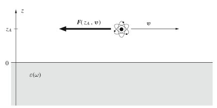
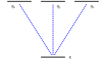
Figure 1: (left) Sketch of the considered geometry. (right) Atomic energy levels.

2.1 Relevant states and observables

The lowest quantum states of the atom are taken by analogy to the ${\rm 1s}$ and ${\rm 2p}$ level of the hydrogen atom: they are denoted $|g\rangle$ for the 1s state, the three degenerate ${\rm 2p}_{i}$ states are written $|\vec{\eta}\rangle$. The unit vector $\vec{\eta}$ is taken from a set $\{\vec{\eta}\}$ forming an orthonormal basis that we may assume real without loss of generality. The Bohr transition frequency between the levels is $\Omega$. We focus in this paper on transitions among these energy levels only and mention briefly where additional states would appear. The nonzero matrix elements of the electric dipole operator $\vec{\hat{D}}(t)$ in the interaction picture are

$$\langle g|\vec{\hat{D}}(t)|\vec{\eta}\rangle=\vec{\eta}\,d\,{\rm e}^{-{\rm i}\Omega t}\,,\qquad\langle\vec{\eta}|\vec{\hat{D}}(t)|g\rangle=\vec{\eta}\,d\,{\rm e}^{{\rm i}\Omega t}~{},$$ (1)

where the transition dipole matrix element $d$ is the basic coupling constant of the field theory. It determines, for example, the static polarizability $\alpha=(2d^{2})/(\hbar\Omega)$ [Eq.(2.2) of Ref.[9]]. Using rotational symmetry, one also has the identity $\sum_{\vec{\eta}}\eta_{i}\eta_{j}=\delta_{ij}$ when the three excited states are summed over.

The atom+field coupling (summation over double indices is assumed hereafter)

$$\hat{V}(t)=-\hat{D}_{i}(t)\hat{E}_{i}(\vec{r}(t),t)=\hat{D}_{i}\partial_{i}\hat{\Phi}(\vec{r}(t),t)$$ (2)

is explicitly time-dependent via the atomic trajectory $\vec{r}(t)$. We will also often use the notation ${\bf r}(t)$ for the path in the $xy$-plane parallel to the surface placed at $z=0$. In our approach the force acting on the atom parallel to this plane is given by the operator [21]

$$\hat{{\bf F}}(t)=\hat{D}_{i}(t)\bfnabla\hat{E}_{i}(\vec{r}(t),t).$$ (3)

More general situations would include higher-order multipole moments of the atomic charge and current distribution (magnetic dipole, electric quadrupole …) and the time derivative of the electromagnetic momentum $\vec{d}\times\vec{B}$. The latter includes the so-called Röntgen interaction that takes into account the transformation of the electromagnetic field into the frame co-moving with the atom. This interaction is relevant at larger (retarded) distances [8].

The field operator is expanded in a plane-wave basis of elementary excitations (photons) and evolves freely according to

$$\hat{\Phi}(\vec{r},t)=\int\!{\rm d}^{2}k\!\int\limits_{0}^{\infty}\!{\rm d}\omega\left(\hat{a}_{{\bf k}\omega}\,\phi_{{\bf k}\omega}\exp({\rm i}{\bf k}\cdot{\bf r}-{\rm i}\omega t)+\mbox{h.c.}\right)~{}.$$ (4)

The bosonic operators satisfy the commutation relation $[\hat{a}^{\phantom{{\dagger}}}_{{\bf k}\omega},\hat{a}^{\dagger}_{{\bf k}^{\prime}\omega^{\prime}}]=\delta({\bf k}-{\bf k}^{\prime})\delta(\omega-\omega^{\prime})$ and the ‘one-photon amplitudes’ are given by [Eq.(2.4) of [9]]

$$\phi_{{\bf k}\omega}=\frac{\sqrt{\omega\Gamma\omega_{p}^{2}/2}}{\omega^{2}+{\rm i}\omega\Gamma-\omega_{S}^{2}}\sqrt{\frac{\hbar}{2\pi^{2}k}}\,{\rm e}^{-kz}~{},$$ (5)

where the frequencies $\omega_{p}$, $\omega_{S}$, and $\Gamma$ parametrize the dielectric function $\varepsilon(\omega)$ of the half-space. We note in particular the relation

$$|\phi_{{\bf k}\omega}|^{2}=\frac{\hbar}{2\pi^{2}}\frac{{\rm e}^{-2kz}}{k}\mathop{\rm Im}R(\omega)=\frac{\hbar}{2\pi^{2}}\frac{{\rm e}^{-2kz}}{k}\mathop{\rm Im}\frac{\varepsilon(\omega)-1}{\varepsilon(\omega)+1}~{},$$ (6)

where $R(\omega)$ is the non-retarded reflection coefficient of the surface. The frequency $\omega_{S}$ gives the surface plasmon resonance and $\Gamma$ its broadening (complex pole of $R(\omega)$). With this expansion for the photon field, the force operator (3), for example, takes the form

$$\hat{{\bf F}}(t) = \int\!{\rm d}^{2}k\int\limits_{0}^{\infty}\!{\rm d}\omega\,\left({\bf k}(\vec{\hat{D}}(t)\cdot\vec{k})\phi_{{\bf k}\omega}\hat{a}_{{\bf k}\omega}\exp({\rm i}{\bf k}\cdot{\bf r}(t)-{\rm i}\omega t)+\mbox{h.c.}\right)~{},$$ (7)

where the three-dimensional wave vector $\vec{k}=({\bf k},{\rm i}k)$ is in fact complex with $\vec{k}\cdot\vec{k}=0$ and $\vec{k}\cdot\vec{k}^{*}=2k^{2}$. Note that this is a ‘skew’ operator that connects quantum states with different photon numbers (for the field) and different energy levels (for the atom).

Since part of our focus will be on the power radiated into photons and pairs of photons, let us introduce

$$P_{1} = \lim_{t\to\infty}\sum_{\vec{\eta}}\int\!{\rm d}^{3}\kappa\,\hbar(\Omega+\omega)\frac{|\langle\vec{\eta},\kappa|\Psi(t)\rangle|^{2}}{t}$$ (8)

$$P_{2} = \frac{1}{2}\lim_{t\to\infty}\int\!{\rm d}^{3}\kappa_{1}\int\!{\rm d}^{3}\kappa_{2}\,\hbar(\omega_{1}+\omega_{2})\frac{|\langle g,\kappa_{1}\kappa_{2}|\Psi(t)\rangle|^{2}}{t}~{},$$ (9)

where $|\langle\vec{\eta},{\bf k}\omega|\Psi(t)\rangle|^{2}$ and $|\langle g,{\bf k}_{1}\omega_{1}{\bf k}_{2}\omega_{2}|\Psi(t)\rangle|^{2}$ are the probabilities of finding the atom in an excited state and one and and the two-photon, respectively (see Secs.2.2 and 4). We also used the compact label $\kappa={\bf k}\omega$ and the factor $\frac{1}{2}$ accounts for double counting the symmetric two-photon states. The long-time limit is to be understood within time-dependent perturbation theory: $t$ is typically not longer than a fraction of the relevant life times. The two-photon power has been calculated in Ref.[9]; we review the evaluation of the integrals in A. This calculation is generalized in Sec.4, where also a partial cancellation between $P_{1}$ and $P_{2}$ is found.

2.2 Atom+field states

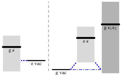
Figure 2: (Color online) Schematic overview of the relevant states for the atom+field theory. The atomic states are labelled ${\rm g}$ and ${\rm e}$ (actually, ${\rm e}$ is threefold degenerate). The notation $\kappa={\bf k}\omega$ collects the quantum numbers of the field states, ${\rm vac}$ is the vacuum state. Two-photon states are denoted $\kappa_{1}\kappa_{2}$. To the left of the vertical dashed line are states that are not directly coupled to the ground state by the atom+field interaction, illustrated by the dotted blue lines. The thick black lines indicate the position of the surface plasmon resonance $\omega_{S}$, the shaded grey area illustrates its broadening (not to scale) over a range $\Gamma$ (intrinsic) and due to the Doppler shift ${\bf k}\cdot{\bf v}$. The Doppler shift is responsible for the appearance of negative frequencies, intuitively understood as measured in the frame co-moving with the atom. The thin dash-dotted line illustrates the two-photon process $g{\rm vac}\leftrightarrow g\kappa_{1}\kappa_{2}$.

In our perturbative approach the initial state is given by the tensor product of atomic ground state and zero photons, $|g,{\rm vac}\rangle$, while the interaction is represented via the operator $\hat{V}(t)$. An expansion up to the third order in the coupling constant $d$ of the atom+field state $|\Psi(t)\rangle$ leads to

$$|\Psi(t)\rangle=(1+c_{0}^{(2)}(t))|g,{\rm vac}\rangle + \sum_{\vec{\eta}}\!\int\!{\rm d}^{3}\kappa\,(c_{1}^{(1)}(t)+c_{1}^{(3)}(t))|\vec{\eta},\kappa\rangle$$ (10)

$$+ \frac{1}{2}\!\int\!{\rm d}^{3}\kappa_{1}\,{\rm d}^{3}\kappa_{2}\,c_{2}^{(2)}(t)|g,\kappa_{1}\kappa_{2}\rangle+\ldots$$

where $c_{n}^{(p)}(t)$ denotes the transition amplitudes for states with $n$ photons in the $p$’th perturbative order and can be obtained by using the standard techniques of perturbation theory. The relevant matrix elements are given by

$$\langle g,{\rm vac}|\hat{V}(t)|\vec{\eta},\kappa\rangle = {\rm i}\,d\,(\vec{\eta}\cdot\vec{k})\phi_{\kappa}\exp[-{\rm i}(\Omega+\omega)t+{\rm i}{\bf k}\cdot{\bf r}(t)]~{},$$ (11)

$$\langle\vec{\eta},\kappa|\hat{V}(t)|g,\kappa_{1}\kappa_{2}\rangle = {\rm i}\,d\,(\vec{\eta}\cdot\vec{k}_{1})\phi_{\kappa_{1}}\,{\rm e}^{{\rm i}(\Omega-\omega_{1})t+{\rm i}{\bf k}_{1}\cdot{\bf r}(t)}\delta(\kappa-\kappa_{2})~{}$$ (12)

$${}+{\rm i}\,d\,(\vec{\eta}\cdot\vec{k}_{2})\phi_{\kappa_{2}}\,{\rm e}^{{\rm i}(\Omega-\omega_{2})t+{\rm i}{\bf k}_{2}\cdot{\bf r}(t)}\delta(\kappa-\kappa_{1})~{},$$

$$\langle\vec{\eta},{\rm vac}|\hat{V}(t)|g,\kappa\rangle = {\rm i}\,d\,(\vec{\eta}\cdot\vec{k})\phi_{\kappa}\exp[{\rm i}(\Omega-\omega)t+{\rm i}{\bf k}\cdot{\bf r}(t)]~{}.$$ (13)

It is important to note that the matrix elements depend on the detail of the path ${\bf r}(t)$. Let consider first the simple case of a constant velocity, i.e. ${\bf r}(t)={\bf v}t$. (Corrections arising from a realistic trajectory including an acceleration stage (‘launch’) are discussed in Sec.4.) In this case time-dependent perturbation theory leads to

$$c_{1}^{(1)}(t) = \frac{{\rm i}\,d\,(\vec{\eta}\cdot\vec{k})^{*}\phi_{\kappa}^{*}}{\hbar(\Omega+\omega^{\prime}-{\rm i}\lambda)}\exp[{\rm i}(\Omega+\omega^{\prime})t]$$ (14)

$$c_{2}^{(2)}(t) = -\frac{d^{2}(\vec{k}_{1}\cdot\vec{k}_{2})^{*}\phi_{\kappa_{1}}^{*}\phi_{\kappa_{2}}^{*}\exp[{\rm i}(\omega_{1}^{\prime}+\omega_{2}^{\prime})t]}{\hbar^{2}(\omega_{1}^{\prime}+\omega_{2}^{\prime}-{\rm i}\lambda)}$$ (15)

$$\qquad\times\bigg{\{}\frac{1}{\Omega+\omega_{1}^{\prime}-{\rm i}\lambda}+\{1\leftrightarrow 2\}\bigg{\}}$$

where the positive infinitesimal $\lambda$ ensures that the atom-field interaction is adiabatically switched on in the past. The scalar product $(\vec{k}_{1}\cdot\vec{k}_{2})^{*}={\bf k}_{1}\cdot{\bf k}_{2}-k_{1}k_{2}$ arises from the summation over the three excited states $|\vec{\eta}\rangle$ and we have used the shorthand $\omega^{\prime}=\omega-{\bf k}\cdot{\bf v}$ for the Doppler-shifted frequency (as ‘seen’ by the moving atom).

The second-order correction $c_{0}^{(2)}(t)$ needs a special handling because it involves the energy shift of the state $|g,{\rm vac}\rangle$ and the rate for the process $|g,{\rm vac}\rangle\to|\vec{\eta},\kappa\rangle$:

$$c_{0}^{(2)}(t)={\rm i}\sum_{\vec{\eta}}\int\!{\rm d}^{3}\kappa\,\frac{d^{2}\,|\vec{\eta}\cdot\vec{k}|^{2}|\phi_{\kappa}|^{2}}{\hbar^{2}(\Omega+\omega-{\bf k}\cdot{\bf v}-{\rm i}\lambda)}\int\limits_{-\infty}^{t}\!{\rm d}t^{\prime}\,{\rm e}^{\lambda t^{\prime}}~{}.$$ (16)

The second integral integral formally evaluates to $\lambda^{-1}{\rm e}^{\lambda t}\approx t+\lambda^{-1}$ for $\lambda\to 0$ so that we identify the frequency shift and inverse lifetime from $1+c_{0}^{(2)}(t)\approx\exp(-{\rm i}\delta E_{g}t/\hbar-\gamma_{g}t/2)$. This yields

$$-{\rm i}\delta E_{g}-\frac{\hbar\gamma_{g}}{2}={\rm i}\sum_{\vec{\eta}}\int\!{\rm d}^{3}\kappa\,\frac{d^{2}\,|\vec{\eta}\cdot\vec{k}|^{2}|\phi_{\kappa}|^{2}}{\hbar(\Omega+\omega-{\bf k}\cdot{\bf v}-{\rm i}\lambda)}~{}.$$ (17)

The level shift $\delta E_{g}$ arising from Eq.(17) has been worked out by Barton, Eq.(3.2) of Ref.[9]. For the lifetime, we get the ‘Golden Rule’ result [30]

$$\gamma_{g}=\frac{2\pi}{\hbar^{2}}\sum_{\vec{\eta}}\int\!{\rm d}^{3}\kappa\,|\langle\vec{\eta},\kappa|\hat{V}|g,{\rm vac}\rangle|^{2}\delta(\Omega+\omega-{\bf k}\cdot{\bf v})~{},$$ (18)

where the atomic motion leads to the Doppler shift of the final photon frequency. This integral is, however, exponentially small for reasonable parameters, as can be seen as follows. The sum over the excited states gives $\sum_{\vec{\eta}}|\vec{\eta}\cdot\vec{k}|^{2}=\vec{k}\cdot\vec{k}^{*}=2k^{2}$. Inserting the coupling strength $|\phi_{\kappa}|^{2}$ from Eq.(6), we get

$$\gamma_{g}=\frac{\alpha\Omega}{\pi}\int\!{\rm d}^{3}\kappa\,k\,{\rm e}^{-2kz}\mathop{\rm Im}R(\omega)\delta(\Omega+\omega-{\bf k}\cdot{\bf v})~{}.$$ (19)

The resonance condition $0=\Omega+\omega-{\bf k}\cdot{\bf v}$ jointly with $\omega\geq 0$ limits the domain for the $k$-integration to ${\bf k}\cdot{\bf v}\geq\Omega$. We then have $k\geq\Omega/v$, and the exponential gives a scaling of this integral proportional to ${\rm e}^{-2\Omega z/v}$. We follow here the same strategy as Ref.[9] and neglect contributions that show such an exponential scaling, assuming that the velocity is small enough: $v\ll\Omega z$. [For a lithium beam at $10\,{\rm keV}$ and $10\,{\rm nm}$ distance, $v/\Omega z\approx 0.02$.] The physical interpretation of this process is the following [see also Ref.[31] in this issue]: the atomic motion leads to an anomalous Doppler shift ($\omega^{\prime}<0$ in the co-moving frame, while $\omega>0$) that makes the ‘spontaneous excitation’ of the ground state possible, similar to Cherenkov radiation [32, 33]. The rate for this process is, however, extremely slow because of the threshold set by the atomic Bohr frequency, $\omega^{\prime}=-\Omega$.

For the third-order correction to the one-photon process one gets:

$$c_{1}^{(3)}(t) = -\frac{{\rm i}}{2\hbar}\int\!{\rm d}^{3}\kappa_{1}\,{\rm d}^{3}\kappa_{2}\int\limits_{-\infty}^{t}\!{\rm d}t^{\prime}\,\langle\vec{\eta},\kappa|\hat{V}(t^{\prime})|g,\kappa_{1}\kappa_{2}\rangle c^{(2)}_{2}(t^{\prime})$$ (20)

$$-\frac{{\rm i}}{\hbar}\int\limits_{-\infty}^{t}\!{\rm d}t^{\prime}\,\langle\vec{\eta},\kappa|\hat{V}(t^{\prime})|g,{\rm vac}\rangle c^{(2)}_{0}(t^{\prime})~{}.$$

Due to the Bose symmetry, the two terms in the matrix element (12) give the same contribution to the first line of (20), and we get

$$c_{1}^{(3)}(t) = \frac{{\rm i}\,d^{3}\phi_{\kappa}^{*}\,{\rm e}^{{\rm i}(\Omega+\omega^{\prime})t}}{\hbar^{3}(\Omega+\omega^{\prime}-{\rm i}\lambda)}\int\!{\rm d}^{3}\kappa_{1}\,\frac{(\vec{\eta}\cdot\vec{k}_{1})|\phi_{\kappa_{1}}|^{2}(\vec{k}_{1}\cdot\vec{k})^{*}}{(\omega_{1}^{\prime}+\omega^{\prime}-{\rm i}\lambda)}$$ (21)

$$\quad\times\bigg{\{}\frac{1}{\Omega+\omega_{1}^{\prime}-{\rm i}\lambda}+\frac{1}{\Omega+\omega^{\prime}-{\rm i}\lambda}\bigg{\}}$$

$$-\frac{{\rm i}\,d(\vec{\eta}\cdot\vec{k})^{*}\phi_{\kappa}^{*}\,{\rm e}^{{\rm i}(\Omega+\omega^{\prime})t}}{\hbar(\Omega+\omega^{\prime}-{\rm i}\lambda)}\Big{(}\frac{\gamma_{g}}{2}+\frac{{\rm i}\delta E_{g}}{\hbar}\Big{)}\Big{(}t+\frac{{\rm i}}{\Omega+\omega^{\prime}-{\rm i}\lambda}\Big{)}~{},$$

where the last line features again a linearly increasing part. This amplitude will be used in Sec.3.2 to calculate the average force operator for an atom in constant motion. A correction $\delta c_{1}^{(3)}(t)$ arising from the acceleration stage is discussed in Sec.4.3 and related to the energy stored in the excited state $|\vec{\eta},\kappa\rangle$.

3 Frictional power and force for constant velocity

The two-photon power $P_{2}$ [Eq.(9)] has been introduced and evaluated in detail in Ref.[9]. There, the calculation was performed for a trajectory where the atom is at rest for $t<0$ and having a constant velocity ${\bf v}$ for $t>0$. We analyze the corresponding process in the following Sec.4, and review an alternative calculation reported in Ref.[8] in Sec.5.2. In this section, we evaluate $P_{2}$ in the case of constant velocity.

3.1 One- and two-photon emission

We find that the only relevant amplitude $c_{2}^{(2)}(t)=\langle g,\kappa_{1}\kappa_{2}|\Psi(t)\rangle$ [Eq.(15)] translates into the following differential emission rate

$${\rm d}w_{2} = \lim_{t\to\infty}\frac{|\langle g,\kappa_{1}\kappa_{2}|\Psi(t)\rangle|^{2}}{t}\frac{{\rm d}^{3}\kappa_{1}\,{\rm d}^{3}\kappa_{2}}{2}$$ (22)

$$= \frac{d^{4}|\vec{k}_{1}\cdot\vec{k}_{2}|^{2}|\phi_{\kappa_{1}}|^{2}|\phi_{\kappa_{2}}|^{2}}{\hbar^{4}}\bigg{|}\frac{1}{\Omega+\omega_{1}^{\prime}}+\{1\leftrightarrow 2\}\bigg{|}^{2}2\pi\delta(\omega_{1}^{\prime}+\omega_{2}^{\prime})\frac{{\rm d}^{3}\kappa_{1}\,{\rm d}^{3}\kappa_{2}}{2}$$

(the factor $1/2$ comes again from the Bose symmetry). This yields, to the fourth order in $d$, the power

$$P_{2}=\frac{d^{4}}{\pi^{3}\hbar}\int \!{\rm d}^{3}\kappa_{1}\,{\rm d}^{3}\kappa_{2}\,\,{\rm e}^{-2(k_{1}+k_{2})z}\frac{|\vec{k}_{1}\cdot\vec{k}_{2}|^{2}}{k_{1}k_{2}}$$ (23)

$${}\times(\omega_{1}+\omega_{2})\mathop{\rm Im}R(\omega_{1})\mathop{\rm Im}R(\omega_{2})\frac{\Omega^{2}\,\delta(\omega_{1}^{\prime}+\omega_{2}^{\prime})}{(\Omega+\omega_{1}^{\prime})^{2}(\Omega+\omega_{2}^{\prime})^{2}}~{}.$$

A simplified evaluation is reviewed in A.2, leading to a scaling $\sim v^{4}$ for a small velocity [Eq.(5.4) of Ref.[9]]:

$$P_{2}\simeq\frac{9}{512\pi}\frac{\hbar v^{4}\alpha^{2}\omega_{p}^{4}\Gamma^{2}}{\omega_{S}^{8}z^{10}}~{}.$$ (24)

Such a scaling with velocity was also found within fluctuation electrodynamics [16, 17, 18], although the numerical prefactor is different. Eqs.(23, 24) coincide exactly with one term in Barton’s results, called there $P_{A}$ (see Eq.(5.4) of Ref.[9]). It is sub-leading, however, compared to another contribution (called $P_{B}$) that scales as ${\cal O}(v^{2})$. Such a leading velocity dependence was also put forward in Refs.[8, 34]. We analyze the origin of the $P_{B}$ contribution of Ref.[9] in Sec.4 where the dependence on the atomic trajectory is pointed out. The calculations of Refs.[8, 18] are reviewed in Secs.5.2, 5.3, respectively.

With respect to the scaling with the frequency parameters for the material response in Eq.(24), a similar behaviour has been observed in previous work on the metal-vacuum surface where the plasmon resonance is at $\omega_{S}=\omega_{p}/\sqrt{2}$ [35, 36, 37]. The combination $\Gamma/\omega_{p}^{2}$ is then proportional to the specific resistance of the metal. Only quasi-DC parameters are relevant for these processes, the spectrum of the plasmon pairs being confined to a region of width $\sim v/z$ around zero frequency.

Since it will play an important role for a generic trajectory [Sec.4], let us also discuss here the one-photon power $P_{1}$. From Eq.(8) we have that to the second order in $d$ it is connected with the squared amplitude $|c_{1}^{(1)}(t)|^{2}$, leading to the differential excitation rate

$${\rm d}w_{1}=\sum_{\vec{\eta}}\frac{d^{2}\,|\vec{\eta}\cdot\vec{k}|^{2}|\phi_{\kappa}|^{2}}{\hbar^{2}}2\pi\delta(\Omega+\omega^{\prime})\,{\rm d}^{3}\kappa~{}.$$ (25)

Summing over all final photon states, we recover exactly the excitation rate $\gamma_{g}$ obtained Eqs.(17, 18). An exponentially small scaling with velocity still holds when the excitation energy is included in the evaluation of $P_{1}^{(2)}=\int\!{\rm d}w_{1}\hbar(\Omega+\omega)$ (the superscript indicates again the perturbative order). A consistent perturbative comparison with $P_{2}$ needs, however, a calculation up to the fourth order in the coupling constant. To evaluate the correction $P_{1}^{(4)}$ to this power in the next order, we consider the mixed term $2\mathop{\rm Re}\,[c_{1}^{(1)*}(t)c_{1}^{(3)}(t)]$ and focus on its most divergent part, namely the one increasing with $t$. We find a decrease of the emission rate:

$$P_{1}^{(4)}\approx-\gamma_{g}tP_{1}^{(2)}~{}.$$ (26)

This suggests the resummation $P_{1}\approx P_{1}^{(2)}\,{\rm e}^{-\gamma_{g}t}$, as expected by the instability of the ground state. This shows that, also to the fourth order, the one-photon power is exponentially suppressed leaving, in the case of a constant velocity, $P_{2}$ and then a force $F\sim v^{3}$ as the only relevant contribution to quantum friction. In Sec.4 we analyze how these results generalize for a more realistic case where the atom, initially at rest, is accelerated to a constant velocity ${\bf v}$.

3.2 Average radiation force

Before proceeding, it is very instructive to directly evaluate the frictional force given in Eq. (3). We consider here the expectation value $\mathbf{F}(t)=\langle\Psi(t)|\hat{\mathbf{F}}(t)|\Psi(t)\rangle$ for an atom in uniform motion parallel to the surface. We shall use again the expansion of the atom+field state $|\Psi(t)\rangle$ up to the third order of the interaction given in Eq.(10). The nonzero matrix elements of the force operator can be derived from Eqs.(11–13): one just needs to replace the prefactor ${\rm i}$ in these equations by ${\bf k}$ or ${\bf k}_{1,2}$. They yield the average force in the form

$$\mathbf{F}(t) = 2\mathop{\rm Re}\Big{\{}\sum_{\vec{\eta}}\!\int\!{\rm d}^{3}\kappa\,\langle g,\mathrm{vac}|\mathbf{\hat{F}}(t)|\vec{\eta},\kappa\rangle(c_{1}^{(1)}(t)+c_{0}^{(2)*}(t)c_{1}^{(1)}(t)+c_{1}^{(3)}(t))$$ (27)

$$+\frac{1}{2}\sum_{\vec{\eta}}\!\int\!{\rm d}^{3}\kappa\,{\rm d}^{3}\kappa_{1}\,{\rm d}^{3}\kappa_{2}\,\langle\vec{\eta},\kappa|\mathbf{\hat{F}}(t)|g,\kappa_{1}\kappa_{2}\rangle c_{1}^{(1)*}(t)c_{2}^{(2)}(t)\Big{\}}~{},$$

where we included products of amplitudes up to order three.

After a straightforward calculation based on Eqs.(14, 15, 16, 21) for the amplitudes $c_{n}^{(p)}(t)$ [details in C], we find that the average force in the long-time limit $t\rightarrow\infty$ can be written as $\mathbf{F}=\mathbf{F}^{(2)}+\mathbf{F}^{(4)}$. The first term

$$\mathbf{F}^{(2)} = -\frac{\hbar\alpha\Omega}{\pi}\!\int\!\mathrm{d}^{3}\kappa\,\mathbf{k}\,k\,\mathrm{e}^{-2kz}\mathop{\rm Im}R(\omega)\delta(\Omega+\omega^{\prime})$$ (28)

is second order in the coupling constant and has a simple interpretation: it is the recoil due to the emission of a photon. This process is accompanied by the excitation of the atom (Cherenkov-Vavilov radiation) and happens at the differential rate ${\rm d}w_{1}$ of Eq.(25). With every emission, the atom receives a momentum $-\hbar{\bf k}$ opposite to the plasmon momentum. The resulting force acting on the atom is $\mathbf{F}=-\int\!{\rm d}w_{1}\,\hbar\mathbf{k}$ which coincides with Eq.(28).

As explained in C, the fourth-order contribution to the force can be presented in the form

$$\mathbf{F}^{(4)} = -\frac{\mathbf{v}}{v^{2}}P_{2}-\gamma_{g}t\,\mathbf{F}^{(2)}-\nabla_{\mathbf{v}}(\gamma_{g}\delta E_{g})+\mbox{other exp. small terms}$$ (29)

where $\gamma_{g}(v)$ and $\delta E_{g}(v)$ are the relaxation rate and Lamb shift of the ground state, respectively, Eq.(17). Recall that $\gamma_{g}(v)$ arises from quantum Cherenkov-Vavilov radiation and is exponentially small. This is also true for the second-order force $\mathbf{F}^{(2)}$ [Eq.(28)] because the resonance condition $\Omega+\omega^{\prime}=0$ involves the same threshold as Eq.(19) for $\gamma_{g}$. The ‘other exp. small’ terms not written explicitly in Eq.(29) have a similar origin.

The important result is that the force (29) gives the leading order for small velocities and involves the two-photon power $P_{2}$ obtained in Eq.(23). This means that for a uniformly moving atom, the average radiation force starts like ${\cal O}(v^{3})$, which is coherent with the radiated power obtained in the previous section. The force calculation thus provides an independent confirmation that two-photon rather than one-photon emission (plus atomic excitation) is the dominant loss process. A comparison with the results of Dedkov and Kyasov [39] and Intravaia et al. [18] is made in A.2: agreement up to a numerical factor is found when the atomic transition is off-detuned with respect to the surface plasmon resonance, $\Omega\ll\omega_{S}$. The dependence on distance involves the steep power law $F\sim 1/z^{10}$.

4 Accelerating the atom and subsequent radiation

In this section, we consider atomic trajectories that are accelerated over a finite duration before reaching their final velocity ${\bf v}$. This material generalizes the calculation of Ref.[9] of the two-photon process where a second term (called $P_{B}$) in the two-photon emission was found that scales with ${\cal O}(v^{2})$ in velocity. The main result is that the term $P_{B}$ depends sensitively on the way the atom is accelerated. Ref.[9] is only recovered for a ‘sudden boost’ (infinitely short duration), while in the opposite or ‘adiabatic’ limit, $P_{B}$ becomes strongly suppressed. The scaling with velocity ${\cal O}(v^{2})$ is maintained, though.

To interpret this behaviour, we have also evaluated the one-photon power $P_{1}$ and found, quite surprisingly, that for accelerated trajectories it is not exponentially small (as in the previous section), it is negative, and exactly cancels the two-photon emission $P_{B}$. This suggests the following picture: the acceleration stage creates a finite occupation $p_{e}\sim v^{2}$ of the excited state (including one photon). The excitation process is qualitatively similar to the ‘acceleration-induced radiative excitation of ground-state atoms’ analyzed by Barton and Calogeracos [38]. Subsequently, this ‘real’ rather than ‘virtual’ excitation decays resonantly into another photon. The resonance condition fixes the energy of the second photon, so that the radiative power captured by the term $P_{B}\sim p_{e}\gamma_{e}\hbar\Omega$ is balanced by a decaying excitation probability (negative $P_{1}$).

The calculation proceeds by working out the probability amplitudes, starting with the one-photon amplitude

$$c_{1}^{(1)}(t) = -\frac{d(\vec{\eta}\cdot\vec{k}^{*})\phi_{\kappa}^{*}}{\hbar}\int\limits_{-\infty}^{t}\!{\rm d}t_{1}\,{\rm e}^{{\rm i}(\Omega+\omega)t_{1}}\,{\rm e}^{-{\rm i}{\bf k}\cdot{\bf r}(t_{1})}~{},$$ (30)

where the matrix element (11) of the atom-field coupling was used. Recall the compact notation $\kappa={\bf k}\omega$ for the photonic modes and note that we have kept a generic atomic path ${\bf r}(t_{1})$ under the integral. The $t_{1}$-integral appearing here will be denoted $\mathcal{A}(e,\kappa;t)$ and discussed in detail in Sec.4.1. We prove there that at large times (once the launch is completed), the amplitude takes the form

$$t\gg\tau:\quad c_{1}^{(1)}(t)\approx-\frac{d(\vec{\eta}\cdot\vec{k}^{*})\phi_{\kappa}^{*}}{\hbar}\bigg{\{}\frac{{\rm e}^{{\rm i}(\Omega+\omega^{\prime})t}}{{\rm i}(\Omega+\omega^{\prime})}+\mathcal{B}_{e,\kappa}\bigg{\}}~{},$$ (31)

where the first term is the same as for a constant-velocity path [Eq.(14)]. We interpret the second term as a non-adiabatic excitation process whose amplitude is approximately (for small velocity) given by

$$\mathcal{B}_{e,\kappa}\approx\frac{{\rm i}\,({\bf k}\cdot{\bf v})\,{\rm e}^{-{\rm i}{\bf k}\cdot{\bf r}(0)}}{(\Omega+\omega)^{2}}\Sigma((\Omega+\omega)\tau)~{}.$$ (32)

The dimensionless factor $\Sigma((\Omega+\omega)\tau)$ depends on the specific shape of the path. It is proportional to the Fourier transform of the acceleration [Eq.(50)] and decays to zero when the product of duration $\tau$ and frequencies $\Omega+\omega$ is much larger than unity. In the opposite limit (‘sudden acceleration’), $\Sigma((\Omega+\omega)\tau)\to 1$.

In the next order of perturbation theory, we deal with the two-photon amplitude

$$c^{(2)}_{2}(t) = -\frac{{\rm i}}{\hbar}\sum_{\vec{\eta}}\int\!{\rm d}\kappa\int\limits_{-\infty}^{t}\!{\rm d}t_{2}\,c_{1}^{(1)}(t_{2})\langle g;\kappa_{1},\kappa_{2}|\hat{V}(t_{2})|\vec{\eta};\kappa\rangle$$

$$= \frac{d^{2}}{\hbar^{2}}(\vec{k}_{1}\cdot\vec{k}_{2})^{*}\phi_{\kappa_{1}}^{*}\phi_{\kappa_{2}}^{*}\int\limits_{-\infty}^{t}\!{\rm d}t_{2}\,\mathcal{A}(e,\kappa_{1};t_{2})\,{\rm e}^{{\rm i}(-\Omega+\omega_{2})t_{2}}\,{\rm e}^{-{\rm i}{\bf k}_{2}\cdot{\bf r}(t_{2})}+\{1\leftrightarrow 2\}~{}.$$

The additional term denoted $\{1\leftrightarrow 2\}$ makes this expression symmetric under plasmon exchange. The $t_{2}$-integral written here will be called $\mathcal{M}_{12}(t)$ similar to Ref.[9]. We find (Sec.4.2) for this two-photon amplitude the asymptotic form

$$t\gg\tau:\quad{\cal M}_{12}(t)\approx-\frac{{\rm e}^{{\rm i}(\omega_{1}^{\prime}+\omega_{2}^{\prime})t}}{(\Omega+\omega_{1}^{\prime})(\omega_{1}^{\prime}+\omega_{2}^{\prime})}+\frac{\mathcal{B}_{e,\kappa_{1}}}{{\rm i}(\omega_{2}^{\prime}-\Omega)}{\rm e}^{{\rm i}(\omega_{2}^{\prime}-\Omega)t}+{\rm cst.}~{},$$ (34)

where the ${\rm cst.}$ denotes $t$-independent terms. The first term again recovers the previous constant-velocity result from Eq.(15). The second term is proportional to the non-adiabatic excitation amplitude ${\cal B}_{e,\kappa}$ [Eqs.(31, 32)] that appeared in the first order.

The power of two-photon emission from Eq.(9) is proportional to $|\mathcal{M}_{12}(t)+\mathcal{M}_{21}(t)|^{2}/t$ in the large-$t$ limit. This is calculated in Eq.(45) below. In Sec.4.3, we finally discuss the rate of change of the energy stored in the excited state $|\vec{\eta},\kappa\rangle$ (the one-photon power $P_{1}$ defined in Eq.(8)) and show that it balances exactly the ${\cal O}(v^{2})$ contribution to the two-photon power.

4.1 Exciting the atom: the one-photon amplitude

Let us consider the first step of the physical process described above. The one-photon transition amplitude is proportional to

$$\mathcal{A}(e,\kappa;t)=\int\limits_{-\infty}^{t}\!{\rm d}t_{1}\;{\rm e}^{i(\Omega+\omega)t_{1}}{\rm e}^{-i{\bf k}\cdot{\bf r}(t_{1})}.$$ (35)

A few general properties of the first-order amplitude can be secured without specifying a particular path. We only require that ${\bf r}(t)$ changes its velocity around $t=0$ with a typical duration $\tau$. We also assume that the origin of the coordinate system is chosen such that for $t\gg\tau$, we have ${\bf r}(t)\approx{\bf v}t$ (see Fig.3 for a sketch). Let us focus first on $t>0$. We split the integral into $-\infty<t_{1}\leq 0$ and $0\leq t_{1}\leq t$, leading to a natural decomposition $\mathcal{A}(t)=\mathcal{A}_{-}+\mathcal{A}_{+}(t)$.

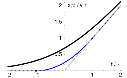
Figure 3: (Color online) Three possible atomic trajectories: smooth continuous boost (thick black line), linear acceleration ramp (thin blue line), and instantaneous boost (dashed gray line). See also the table below for more detail.

Curve	$\dot{x}(t)$	$\ddot{x}(t)$
thick black	$v/(1+{\rm e}^{-t/\tau})$	$v\tau^{-1}/(2+2\cosh t/\tau)$
thin blue	$\left\{\begin{array}[]{ll}0&\mbox{for $t<-\tau$}\\ (t+\tau)v/(2\tau)&\mbox{for $-\tau<t<\tau$}\\ v&\mbox{for $t>\tau$}\end{array}\right.$	$\left\{\begin{array}[]{ll}0&\mbox{for $t<-\tau$}\\ v/(2\tau)&\mbox{for $-\tau<t<\tau$}\\ 0&\mbox{for $t>\tau$}\end{array}\right.$
dashed gray	$\left\{\begin{array}[]{ll}0&\mbox{for $t<0$}\\ v&\mbox{for $t>0$}\end{array}\right.$	$v\delta(t)$

For the term $\mathcal{A}_{+}(t)$, we perform a partial integration after subtracting and adding ${\bf v}t_{1}$ in the exponent [see Eq.(30)]. This leads to

$$\mathcal{A}_{+}(t)=\left.\frac{{\rm e}^{{\rm i}(\Omega+\omega)t_{1}}\,{\rm e}^{-{\rm i}{\bf k}\cdot{\bf r}(t_{1})}}{{\rm i}(\Omega+\omega-{\bf k}\cdot{\bf v})}\right|^{t}_{0}+\int\limits_{0}^{t}\!{\rm d}t_{1}\frac{{\bf k}\cdot(\dot{\bf r}-{\bf v})}{\Omega+\omega-{\bf k}\cdot{\bf v}}{\rm e}^{{\rm i}(\Omega+\omega)t_{1}}\,{\rm e}^{-{\rm i}{\bf k}\cdot{\bf r}(t_{1})}~{}.$$ (36)

The advantage of this representation is that the first term yields what we call the ‘adiabatic limit’

$$\mathcal{A}_{+}^{({\rm ad})}(e,\kappa;t)=\frac{{\rm e}^{{\rm i}(\Omega+\omega)t}\,{\rm e}^{-{\rm i}{\bf k}\cdot{\bf r}(t)}}{{\rm i}(\Omega+\omega-{\bf k}\cdot{\bf v})}$$ (37)

which is nothing but the term we found previously for a trajectory with constant velocity [see Eq.(14)]. In the integrand in Eq.(36), the difference $\dot{\bf r}-{\bf v}$ vanishes as soon as the atom has reached a constant velocity. Hence the integral approaches a constant for $t\gg\tau$. In this limit, we therefore proved that the excitation amplitude takes the form

$$t\gg\tau:\qquad\mathcal{A}(e,\kappa;t)=\mathcal{A}_{+}^{({\rm ad})}(e,\kappa;t)+\mathcal{B}_{e,\kappa}+o(1)~{},$$ (38)

where $\mathcal{B}_{e,\kappa}$ can be read off by adding $\mathcal{A}_{-}$ to the remaining terms in Eq.(36). The error $o(1)$ in Eq.(38) is made of terms that vanish in the limit $t\gg\tau$. A similar manipulation can be applied when $t\leq 0$. No splitting and subtraction are needed, and we get

$$t\leq 0:\qquad\mathcal{A}(e,\kappa;t)=\frac{{\rm e}^{{\rm i}(\Omega+\omega)t}\,{\rm e}^{-{\rm i}{\bf k}\cdot{\bf r}(t)}}{{\rm i}(\Omega+\omega)}+\int\limits_{-\infty}^{t}\!{\rm d}t_{1}\frac{{\bf k}\cdot\dot{\bf r}}{\Omega+\omega}{\rm e}^{{\rm i}(\Omega+\omega)t_{1}}\,{\rm e}^{-{\rm i}{\bf k}\cdot{\bf r}(t_{1})}~{}.$$ (39)

The first term may again be called ‘adiabatic’ and does not contain any contribution from the lower limit $t=-\infty$ because we assume that the atom-field coupling is switched off there. Note also that there is no Doppler shift in the frequency denominator. The second term vanishes for $t\ll-\tau$ when the atom is still at rest.

4.2 Emitting the second photon

Here, we focus on the two-photon amplitude in the long-time limit $t\to\infty$. Using the time scale $\tau$ for the ‘acceleration stage’ of the atomic trajectory, we assume more specifically $t\gg\tau$. Let us introduce a time $t_{a}$ with the property $\tau\ll t_{a}\ll t$ such that the atomic velocity is $\dot{\bf r}(t_{a})={\bf v}$. We split the integration range of the $t_{2}$-integral in Eq.(4) into $-\infty<t_{2}<t_{a}$ and into $t_{a}<t_{2}<t$ obtaining $\mathcal{M}_{12}(t)=\mathcal{M}_{-}+\mathcal{M}_{+}(t)$ (and similarly for $\mathcal{M}_{21}(t)$). We shall see that only the probability $|\mathcal{M}_{+}(t)|^{2}$ contains terms growing linearly with $t$ and then contributing to the radiated power, while the rest tends towards a constant. The contribution ${\cal M}_{+}(t)$ can be evaluated by inserting the asymptotic form (38) for the amplitude ${\cal A}(e,\kappa_{1};t)$ into the integral:

$${\cal M}_{+}(t) = \int\limits_{t_{a}}^{t}\!{\rm d}t_{2}\,\left(\mathcal{A}_{+}^{({\rm ad})}(e,\kappa_{1};t_{2})+\mathcal{B}_{e,\kappa_{1}}\right){\rm e}^{{\rm i}(\omega_{2}-\Omega)t_{2}}\,{\rm e}^{-{\rm i}{\bf k}_{2}\cdot{\bf r}(t_{2})}$$ (40)

$$= {\cal M}_{+}^{(A)}(t)+{\cal M}_{+}^{(B)}(t).$$

Because, for $t>t_{a}$, the atomic velocity is constant and the first term evaluates to

$${\cal M}_{+}^{(A)}(t)=-\left.\frac{{\rm e}^{{\rm i}(\omega_{1}^{\prime}+\omega_{2}^{\prime})t_{2}}}{(\Omega+\omega_{1}^{\prime})(\omega_{1}^{\prime}+\omega_{2}^{\prime})}\right|^{t}_{t_{a}},\quad(\omega_{i}^{\prime}=\omega_{i}-{\bf k}_{1}\cdot{\bf v})$$ (41)

we recover the result for a constant velocity [cf. Eq.(15)]. We symmetrize under photon exchange, square and get in the limit $t\gg t_{a}$:

$$\left|{\cal M}_{+}^{(A)}(t)+\{1\leftrightarrow 2\}\right|^{2}=2\pi(t-t_{a})\delta(\omega_{1}^{\prime}+\omega_{2}^{\prime})\frac{(2\Omega+\omega_{1}^{\prime}+\omega_{2}^{\prime})^{2}}{(\Omega+\omega_{1}^{\prime})^{2}(\Omega+\omega_{2}^{\prime})^{2}}~{},$$ (42)

where the sum $\omega_{1}^{\prime}+\omega_{2}^{\prime}$ in the numerator can of course be omitted. The second term ${\cal M}_{+}^{(B)}(t)$ in Eq.(40) is an elementary integral as well:

$${\cal M}_{+}^{(B)}(t)=\frac{\mathcal{B}_{e,\kappa_{1}}}{{\rm i}(\omega_{2}^{\prime}-\Omega)}\left.{\rm e}^{{\rm i}(\omega_{2}^{\prime}-\Omega)t_{2}}\right|^{t}_{t_{a}}~{}.$$ (43)

We symmetrize again and identify the individual squares as the leading terms:

$$\left|{\cal M}_{+}^{(B)}(t)+\{1\leftrightarrow 2\}\right|^{2}=2\pi(t-t_{a})\delta(\omega_{2}-\Omega)|\mathcal{B}_{e,\kappa_{1}}|^{2}+\{1\leftrightarrow 2\}~{}.$$ (44)

It can be checked that the ‘mixed terms’ in the squared amplitude lead to contributions that either oscillate or tend to constants as $t\to\infty$ (no inverse squares like $1/(\omega_{1}^{\prime}+\omega_{2}^{\prime})^{2}$ appear). This also holds true for the mixed terms involving one factor ${\cal M}_{-}$ (see B for more details). Finally we get

$$\lim_{t\rightarrow\infty}\frac{|{\cal M}_{12}(t)+{\cal M}_{21}(t)|^{2}}{t} = 2\pi\delta(\omega_{1}^{\prime}+\omega_{2}^{\prime})\frac{4\Omega^{2}}{(\Omega+\omega_{1}^{\prime})^{2}(\Omega+\omega_{1}^{\prime})^{2}}$$ (45)

$$+2\pi\delta(\omega_{2}^{\prime}-\Omega)\left|\mathcal{B}_{e,\kappa_{1}}\right|^{2}+\{1\leftrightarrow 2\}~{}.$$

From the above calculation, one can see that the first line of Eq.(45) involves only the constant-velocity part of the atomic path and hence does not depend on the way the atom is put into motion. As was reviewed in Sec.3 and A.2, this term contributes the amount $P_{A}\sim v^{4}$ to the two-photon emission. The second line of Eq.(45) leads to

$$P_{B}=\frac{\alpha^{2}\Omega^{2}}{4\hbar}\int\!{\rm d}^{3}\kappa_{1}\,{\rm d}^{3}\kappa_{2}\,(\omega_{1}+\omega_{2})|\vec{k}_{1}\cdot\vec{k}_{2}|^{2}|\phi_{1}\phi_{2}|^{2}2\pi\delta(\omega_{2}-\Omega)|\mathcal{B}_{e,\kappa_{1}}|^{2}$$ (46)

and scales with $v^{2}$ for small velocity [A.1]. This arises because the amplitude $\mathcal{B}_{e,\kappa}\sim v$, as we now show.

We start with the general expression collected from the terms in Eqs.(36, 39) that become constants for large $t\gg\tau$:

$$\mathcal{B}_{e,\kappa} = \frac{{\rm e}^{-{\rm i}{\bf k}\cdot{\bf r}(0)}}{{\rm i}(\Omega+\omega)}+\int\limits_{-\infty}^{0}\!{\rm d}t_{1}\frac{{\bf k}\cdot\dot{\bf r}}{\Omega+\omega}{\rm e}^{{\rm i}(\Omega+\omega)t_{1}}\,{\rm e}^{-{\rm i}{\bf k}\cdot{\bf r}(t_{1})}$$ (47)

$${}-\frac{{\rm e}^{-{\rm i}{\bf k}\cdot{\bf r}(0)}}{{\rm i}(\Omega+\omega-{\bf k}\cdot{\bf v})}+\int\limits_{0}^{\infty}\!{\rm d}t_{1}\frac{{\bf k}\cdot(\dot{\bf r}-{\bf v})}{\Omega+\omega-{\bf k}\cdot{\bf v}}{\rm e}^{{\rm i}(\Omega+\omega)t_{1}}\,{\rm e}^{-{\rm i}{\bf k}\cdot{\bf r}(t_{1})}~{}.$$

The first terms in the two lines sum to

$$\frac{{\rm e}^{-{\rm i}{\bf k}\cdot{\bf r}(0)}}{{\rm i}(\Omega+\omega)}-\frac{{\rm e}^{-{\rm i}{\bf k}\cdot{\bf r}(0)}}{{\rm i}(\Omega+\omega-{\bf k}\cdot{\bf v})}=\frac{(-{\bf k}\cdot{\bf v})\,{\rm e}^{-{\rm i}{\bf k}\cdot{\bf r}(0)}}{{\rm i}(\Omega+\omega)(\Omega+\omega-{\bf k}\cdot{\bf v})}~{}.$$ (48)

This is also what is found for Ref.[9]’s ‘kink trajectory’ where $\dot{\bf r}=0$ for $t<0$ and $\dot{\bf r}={\bf v}$ for $t>0$. The remaining integrals are bounded by ${\cal O}(kv\tau/(\Omega+\omega))$ so that their contribution to the amplitude $\mathcal{B}_{e,\kappa}$ is also linear in the velocity $v$. To proceed, we apply another partial integration to the two integrals in Eq.(47). Summing the results and expanding for small $v$, one gets

$$\int\limits_{-\infty}^{0}\!{\rm d}t_{1}\frac{{\bf k}\cdot\dot{\bf r}}{\Omega+\omega}{\rm e}^{{\rm i}(\Omega+\omega)t_{1}}\,{\rm e}^{-{\rm i}{\bf k}\cdot{\bf r}(t_{1})}+\int\limits_{0}^{\infty}\!{\rm d}t_{1}\frac{{\bf k}\cdot(\dot{\bf r}-{\bf v})}{\Omega+\omega-{\bf k}\cdot{\bf v}}{\rm e}^{{\rm i}(\Omega+\omega)t_{1}}\,{\rm e}^{-{\rm i}{\bf k}\cdot{\bf r}(t_{1})}$$

$$\approx\frac{{\bf k}\cdot{\bf v}\,{\rm e}^{-{\rm i}{\bf k}\cdot{\bf r}(0)}}{{\rm i}(\Omega+\omega)^{2}}-\frac{{\rm e}^{-{\rm i}{\bf k}\cdot{\bf r}(0)}}{{\rm i}(\Omega+\omega)^{2}}\!\int\limits_{-\infty}^{\infty}\!{\rm d}t_{1}{\bf k}\cdot\ddot{\bf r}\,{\rm e}^{{\rm i}(\Omega+\omega)t_{1}}$$ (49)

where the first term cancels with (48) to leading order in $v$. We are thus left with the Fourier integral of the atomic acceleration

$$\mathcal{B}_{e,\kappa}\approx-\frac{{\rm e}^{-{\rm i}{\bf k}\cdot{\bf r}(0)}}{{\rm i}(\Omega+\omega)^{2}}\!\int\limits_{-\infty}^{\infty}\!{\rm d}t_{1}{\bf k}\cdot\ddot{\bf r}(t_{1})\,{\rm e}^{{\rm i}(\Omega+\omega)t_{1}}=\frac{{\rm i}\,({\bf k}\cdot{\bf v})\,{\rm e}^{-{\rm i}{\bf k}\cdot{\bf r}(0)}}{(\Omega+\omega)^{2}}\Sigma((\Omega+\omega)\tau)~{}.$$ (50)

which is the result announced in Eq.(32). This already permits us to draw a conclusion for a generic trajectory whose velocity is monotonously raised to its final value ${\bf v}$. The Fourier transform of the acceleration then exists and is maximal for $\Omega+\omega=0$. If the acceleration occurs over a finite duration ${\cal O}(\tau)$, the Fourier transform drops to zero when the frequencies satisfy $(\Omega+\omega)\tau\gg 1$. On physical grounds, it seems quite plausible that the acceleration stage takes more than a few femtoseconds while $\Omega$ is typically in the visible range (and $\omega>0$). This inequality is therefore amply satisfied, and the corresponding two-photon emission is strongly suppressed.

It is interesting to examine different atomic trajectories ${\bf r}(t)$ and provide a quantitative analysis how the ‘acceleration stage’ affects the final result for the two-photon emission $P_{B}$. A trivial example to begin with is an inertial path with constant velocity. The acceleration is zero at all times, and Eq.(50) gives ${\cal B}_{e,\kappa}=0$. Hence the two-photon power $P_{B}=0$, and only the ${\cal O}(v^{4})$ contribution called $P_{A}$ from Sec.3 remains.

Our second example is Ref.[9]’s instantaneous boost, $\ddot{\bf r}(t)={\bf v}\delta(t)$. The trajectory is plotted as a dashed line in Fig.3. The Fourier integral gives

$$|\mathcal{B}_{e,\kappa}|^{2}\approx\frac{({\bf k}\cdot{\bf v})^{2}}{(\Omega+\omega)^{4}}.$$ (51)

This result can also been inferred from Eq.(4.10) of Ref.[9] by writing it in the form given in Eq.(45) (and taking into account the erratum).

As a third example, consider a linear velocity ramp, as illustrated by the middle path in Fig.3. Velocity and acceleration are given in the caption: specifically the acceleration is constant during an interval of length $2\tau$ (details of the full calculation for this path can be found in B). The sinc-function resulting from the Fourier integral (50) then gives

$$|\mathcal{B}_{e,\kappa}|^{2}\approx\frac{({\bf k}\cdot{\bf v})^{2}}{(\Omega+\omega)^{4}}\frac{\sin^{2}[(\Omega+\omega)\tau]}{(\Omega+\omega)^{2}\tau^{2}}~{}.$$ (52)

The second fraction reproduces Ref.[9]’s path in the limit $\tau\to 0$, but gives a strong reduction in the opposite case. Since the typical frequencies contributing to the integral (46) are $\omega_{1}\simeq\omega_{S}$ due to the plasmon pole, $|\phi_{1}|^{2}\sim\mathop{\rm Im}R(\omega_{1})$, the power $P_{B}$ gets reduced by a factor $1/(\tau(\Omega+\omega_{S}))^{2}\ll 1$. This result for the linear velocity ramp has been reproduced through a differently routed calculation by G. Barton (private communication).

Finally, let us consider the ‘smooth boost’ plotted as a thick black line in Fig.3. The acceleration is given by an infinitely differentiable function (see figure caption) whose maximum value is $v/(4\tau)$ and whose width is ${\cal O}(\tau)$. Evaluating its Fourier transform, we get the probability

$$|{\cal B}_{e,\kappa}|^{2}=\frac{({\bf k}\cdot{\bf v})^{2}}{(\Omega+\omega)^{4}}\left[\frac{\pi(\Omega+\omega)\tau}{\sinh[\pi(\Omega+\omega)\tau]}\right]^{2}~{}.$$ (53)

The second fraction in this expression shows that compared to the ‘kink path’, the power $P_{B}$ becomes exponentially small in the limit of an adiabatic boost $\tau\Omega\gg 1$.

Let us attach a physical meaning to the quantities calculated in the previous sections. Going back to the Schrödinger picture, the first-order amplitude $c_{1}^{(1)}(t)$ [Eq.(31)] takes the form

$$c_{1}^{(1)}(t)\approx-\frac{d(\vec{\eta}\cdot\vec{k}^{*})\phi_{\kappa}^{*}}{\hbar}\bigg{\{}\frac{1}{{\rm i}(\Omega+\omega^{\prime})}+\mathcal{B}_{e,\kappa}\,{\rm e}^{-{\rm i}(\Omega+\omega^{\prime})t}\bigg{\}}~{}.$$ (54)

The first term, independent of $t$, can be understood as being part of the (‘dressed’) ground state $|g,{\rm vac}\rangle$ (still at zero energy), where the atom is surrounded by a (‘virtual’) cloud of photons (plasmons). The second term oscillates at the (bare) energy of the excited state $|\vec{\eta},\kappa\rangle$, but including the Doppler shift ($\omega^{\prime}$ instead of $\omega$). It can be shown that the Hamiltonian of our atom+field theory can be transformed to a time-independent form by going into a frame moving with the atom. (Details are postponed to another paper.) In this picture, the state $|\vec{\eta},\kappa\rangle$ evolves freely at the frequency $\Omega+\omega^{\prime}$. We therefore conjecture that along a path with a time-dependent acceleration, the amplitude $\mathcal{B}_{e,\kappa}$ describes the ‘real’ excitation of the atom+field system [38]. The required energy transfer is in heuristic agreement with the frequency uncertainty arising from the finite duration of the acceleration, as expressed in the Fourier integral (50).

We can also define an excitation probability (not a rate), summing over the plasmon states and the three sublevels $|\vec{\eta}\rangle$

$$p_{e} = \sum_{\vec{\eta}}\frac{d^{2}}{\hbar^{2}}\int\!{\rm d}^{3}\kappa\,|\vec{\eta}\cdot\vec{k}|^{2}|\phi_{\kappa}|^{2}|\mathcal{B}_{e,\kappa}|^{2}$$ (55)

$$= \frac{\alpha\Omega}{2\pi^{2}}\int\!{\rm d}^{3}\kappa\,k\,{\rm e}^{-2kz}\mathop{\rm Im}R(\omega)\frac{({\bf k}\cdot{\bf v})^{2}}{(\Omega+\omega)^{4}}|\Sigma((\Omega+\omega)\tau)|^{2}~{}.$$

where the $k$-integral can be performed, yielding $3\pi v^{2}/(4z^{5})$.

4.3 Excitation power: a subtle cancellation to the fourth order

The previous analysis examined in detail all the components of the physical process describing the acceleration, the excitation and the subsequent radiation of an atom in motion near a surface. This was necessary in order to discern and generalize, to the case of a generic trajectory, each single contribution to quantum friction. In Ref.[9] the friction force ${\bf F}$ is calculated based on the identification with the two-photon power loss, $P_{2}=-{\bf v}\cdot{\bf F}$. For a generic trajectory this calculation led to $P_{2}=P_{A}+P_{B}$ where $P_{B}\sim{\cal O}(v^{2})$ gives the leading order. Barton thus concludes that ${\bf F}\sim v$ for small velocity [9], at least for the trajectory called instantaneous boost above. In the last section we showed, however, that the value of $P_{B}$ depends on the detail of the trajectory: a smooth boost gives a significant reduction, and a constant velocity simply leads to $P_{B}=0$ (see also Sec.3).

Although physically sounding, the calculation based on $P_{2}$ is incomplete since it does not take into account the power needed to create the excited state $|\vec{\eta},\kappa\rangle$, called the one-photon power $P_{1}$ in Eq.(8). A similar omission in earlier work was criticized by Volokitin and Persson, see Ref.[13]. (For an analysis of the ‘internal energy’ appearing in $P_{1}$, see also Ref.[39], for example.) The sum $P_{1}+P_{2}$ translates the change in the total energy of the evolving state $|\Psi(t)\rangle$. This energy is not conserved, since the interaction is time-dependent. For the same reason, only the free Hamiltonian $\hat{H}_{0}=\hat{H}_{A}+\hat{H}_{F}$ (atom and field) is used to define the energy of the state $|\Psi(t)\rangle$:

$$\langle\Psi(t)|\hat{H}_{0}|\Psi(t)\rangle\approx t(P_{1}+P_{2})+\ldots$$ (56)

The power $P_{1}$ is calculated again by pushing to the third order the one-photon amplitude $\langle\vec{\eta},\kappa|\Psi(t)\rangle$, called $c_{1}^{(3)}(t)$ in Eq.(10). This extension is necessary because at first order, even with an acceleration phase, the excitation rate is exponentially small [see Eq.(19)]. We focus again on the state sequence $|g,{\rm vac}\rangle\to|\vec{\eta},\kappa\rangle\to|g,\kappa_{1}\kappa_{2}\rangle\to|\vec{\eta},\kappa\rangle$ passing via the two-photon state. (The sequence via the ground state $|g,{\rm vac}\rangle$ gives again exponentially small contributions.)

The calculation proceeds along lines similar to Sec.3. Perturbation theory yields the integral (20) where we insert now the expression for $\langle g,\kappa_{1}\kappa_{2}|\Psi(t)\rangle$ generalized to the case of a generic trajectory (proportional to the amplitude ${\cal M}(t)$ from Sec.4.2). In addition to the constant velocity result we obtain a correction $\delta c_{1}^{(3)}(t)$ to the amplitude coming from the second term in Eq.(34) and its symmetrized partner. We consider that interaction times in the interval $\tau<t_{3}<t$ give the main contribution and approximate

$$\delta c_{1}^{(3)}(t) \approx \frac{d^{3}}{\hbar^{3}}\int\!{\rm d}^{3}\kappa_{1}\!(\vec{k}_{1}\cdot\vec{k})^{*}|\phi_{\kappa_{1}}|^{2}\phi_{\kappa}^{*}(\vec{\eta}\cdot\vec{k}_{1})$$ (57)

$$\quad{}\times\int\limits_{\tau}^{t}\!{\rm d}t_{3}\bigg{\{}\frac{{\cal B}_{e,\kappa_{1}}\,{\rm e}^{{\rm i}(\omega^{\prime}-\omega_{1}^{\prime})t_{3}}}{{\rm i}(\omega^{\prime}-\Omega-{\rm i}\lambda)}+\frac{{\cal B}_{e,\kappa}}{{\rm i}(\omega^{\prime}_{1}-\Omega-{\rm i}\lambda)}\bigg{\}}~{}.$$

The second term in the curly brackets gives rise to a linear increase in time. The fourth-order approximation to the excited-state probability $|\langle\vec{\eta},\kappa|\Psi(t)\rangle|^{2}\approx|c_{1}^{(1)}(t)|^{2}+2\mathop{\rm Re}[c_{1}^{(1)*}(t)\delta c_{1}^{(3)}(t)]+\ldots$ thus provides us with an excitation rate

$$\lim_{t\to\infty}\frac{|\langle\vec{\eta},\kappa|\Psi(t)\rangle|^{2}-|c_{1}^{(1)}(t)|^{2}}{t}$$

$$\approx-\frac{2d^{4}}{\hbar^{4}}\mathop{\rm Re}\bigg{[}(\vec{\eta}\cdot\vec{k})|\phi_{\kappa}|^{2}\int\!{\rm d}^{3}\kappa_{1}\!(\vec{k}_{1}\cdot\vec{k})^{*}|\phi_{\kappa_{1}}|^{2}(\vec{\eta}\cdot\vec{k}_{1})\frac{|{\cal B}_{e,\kappa}|^{2}}{{\rm i}(\omega^{\prime}_{1}-\Omega-{\rm i}\lambda)}\bigg{]}~{}.$$ (58)

Note that for this rate of change, we only need the non-adiabatic amplitude ${\cal B}_{e,\kappa}$ in the first-order expression $c_{1}^{(1)*}(t)$ [Eq.(31)], since the other combinations give rise to oscillating contributions. The one-photon power (8) becomes

$$P_{1}=-\frac{\alpha^{2}\Omega^{2}}{4\hbar}\int\!{\rm d}^{3}\kappa\,{\rm d}^{3}\kappa_{1}\!(\Omega+\omega)|\phi_{\kappa}|^{2}|\phi_{\kappa_{1}}|^{2}|\vec{k}_{1}\cdot\vec{k}|^{2}|{\cal B}_{e,\kappa}|^{2}2\pi\delta(\omega^{\prime}_{1}-\Omega)~{}.$$ (59)

To the lowest order in velocity (recall that ${\cal B}_{e,\kappa}$ is proportional to $v$), we may drop the Doppler shift in $\delta(\omega^{\prime}_{1}-\Omega)$. Now, it is possible to check that the one-photon power (59) exactly balances the contribution $P_{B}$ to the two-photon power [Eq.(46)]. It leaves $P_{A}$ as the only relevant contribution for the total dissipated power, even for a particle path including an acceleration phase.

The work developed in this section is the central result of our paper. Firstly, it shows that the perturbative approach described in Ref.[9] strongly depends on the acceleration phase that brings the atom to a constant velocity $v$. Secondly, it proves that the description given in Ref.[9] of the quantum friction is incomplete and that, when corrected, it is in agreement with a drag force at zero temperature proportional to $v^{3}$.

5 Results from fluctuation electrodynamics

In the previous sections we provided a complete description of quantum friction within the framework of perturbation theory. This approach has the merit of relying on well-established techniques, even if the mathematical machinery is somewhat cumbersome. Quantum friction, however, has been examined within other frameworks, approaching the problem from other perspectives. For the sake of completeness, we review in this section some of the results from fluctuation electrodynamics, which is one of the most used approaches to describe the quantum mechanical interaction of two neutral objects.

5.1 Spectral densities

Correlation functions of the atom and field variables are a convenient way to characterize the atom-field interaction in terms of ‘resonant’ and ‘non-resonant’ processes. We start by collecting a few formulas for the free observables and evaluate their correlations in the ‘bare’ ground state denoted as $|g,{\rm vac}\rangle$.

Field correlations.

We use ‘time-ordered’ correlations as they often appear in time-dependent perturbation theory. For the free scalar potential and $t>t^{\prime}$

$$C_{\Phi}(\vec{r},\vec{r}\,^{\prime}\!,t-t^{\prime})=\langle{\rm vac}|\hat{\Phi}(\vec{r},t)\hat{\Phi}(\vec{r}\,^{\prime}\!,t^{\prime})|{\rm vac}\rangle$$

$$=\frac{\hbar}{2\pi^{2}}\int\!\frac{{\rm d}^{2}k}{k}\!\int\limits_{0}^{\infty}\!{\rm d}\omega\,\mathop{\rm Im}R(\omega){\rm e}^{{\rm i}{\bf k}\cdot({\bf r}-{\bf r}^{\prime})-k(z+z^{\prime})}{\rm e}^{-{\rm i}\omega(t-t^{\prime})}~{}.$$ (60)

Evaluating this for an atom with constant velocity ${\bf v}$, we get ${\bf r}(t)-{\bf r}(t^{\prime})=(t-t^{\prime}){\bf v}$ and observe that the vacuum spectrum extends into negative frequencies, of the order ${\cal O}(-{\bf k}\cdot{\bf v})={\cal O}(-{v}/z)$. This estimate is based on the natural momentum cutoff provided by the exponential ${\rm e}^{-k(z+z^{\prime})}$. The rest of the frequency dependence is governed by the reflection amplitude $R(\omega)$: a peak at the surface plasmon resonance $\omega=\omega_{S}$ with width $\Gamma$ and an algebraic decay $\sim 1/\omega^{3}$ in the UV. In the time domain, these features translate into a correlation that oscillates at $\omega_{S}$ with an exponential envelope of width $1/\Gamma$, plus an algebraic long-term tail $\sim 1/(t-t^{\prime})^{2}$ that arises from the ‘Ohmic’ behavior $\mathop{\rm Im}R(\omega)\sim\omega$ for $\omega\to 0$. For the electric field, evaluated along an atomic path parallel to the surface, we get similarly ($\omega^{\prime}=\omega-{\bf k}\cdot{\bf v}$, frequency in the co-moving frame)

$$\langle{\rm vac}|\hat{E}_{i}(\vec{r}(t),t)\hat{E}_{j}(\vec{r}(t^{\prime}),t^{\prime})|{\rm vac}\rangle$$

$$=\frac{\hbar}{2\pi^{2}}\int\!{\rm d}^{2}k\frac{k_{i}k_{j}^{*}\,{\rm e}^{-2kz}}{k}\!\int\limits_{-{\bf k}\cdot{\bf v}}^{\infty}\!{\rm d}\omega^{\prime}\,\mathop{\rm Im}R(\omega^{\prime}+{\bf k}\cdot{\bf v}){\rm e}^{-{\rm i}\omega^{\prime}(t-t^{\prime})}~{}.$$ (61)

Note that for a more general trajectory, the correlations are not stationary, and more involved spectral representations like Wigner or wavelet transforms would be needed. The response function of the free field is known as the Green function (tensor). Standard linear response theory gives

$$G_{ij}(\vec{r},\vec{r}\,^{\prime}\!,t-t^{\prime}) = \frac{{\rm i}}{\hbar}\Theta(t-t^{\prime})\langle{\rm vac}|\big{[}\hat{E}_{i}(\vec{r},t),\hat{E}_{j}(\vec{r}\,^{\prime}\!,t^{\prime})\big{]}|{\rm vac}\rangle$$ (62)

$$= \frac{{\rm i}}{2\pi^{2}}\Theta(t-t^{\prime})\int\!{\rm d}^{2}k\frac{{\rm e}^{-k(z+z^{\prime})}}{k}\,{\rm e}^{{\rm i}{\bf k}\cdot({\bf r}-{\bf r}^{\prime})}$$

$${}\times\int\limits_{0}^{\infty}\!{\rm d}\omega\,\mathop{\rm Im}R(\omega)\big{[}k_{i}k_{j}^{*}\,{\rm e}^{-{\rm i}\omega(t-t^{\prime})}-k_{j}k_{i}^{*}\,{\rm e}^{{\rm i}\omega(t-t^{\prime})}\big{]}$$

with an obvious evaluation along the path of a moving atom. ( It can be checked that the last line of Eq.(62) agrees with the solution of the Maxwell equations for a point dipole in the non-retarded approximation.)

Dipole correlations.

The free dipole operator shows in the theory of Ref.[9] a sharp line. It is actually the specific challenge of this model that the line broadening appears self-consistently at higher orders in perturbation theory. In the atomic ground state

$$\langle g|\hat{D}_{i}(t)\hat{D}_{j}(t^{\prime})|g\rangle^{(0)}=\delta_{ij}\frac{\hbar\alpha\Omega}{2}\,{\rm e}^{-{\rm i}\Omega(t-t^{\prime})}$$ (63)

after summing over the degenerate excited states $|\vec{\eta}\rangle$. In a simple scheme where the states $|\vec{\eta}\rangle$ have decay rates $\gamma_{\vec{\eta}}$, this could be generalized to

$$\langle g|\hat{D}_{i}(t)\hat{D}_{j}(t^{\prime})|g\rangle\approx\frac{\hbar\alpha\Omega}{2}\sum_{\vec{\eta}}\eta_{i}\eta_{j}\,{\rm e}^{-{\rm i}\Omega(t-t^{\prime})-\gamma_{\vec{\eta}}|t-t^{\prime}|/2}$$ (64)

giving a Lorentzian spectrum:

$$S_{ij}(\omega)=\int\!{\rm d}\tau\,{\rm e}^{{\rm i}\omega\tau}\langle g|\hat{D}_{i}(t+\tau)\hat{D}_{j}(t)|g\rangle=\frac{\hbar\alpha\Omega}{2}\sum_{\vec{\eta}}\frac{\gamma_{\vec{\eta}}\,\eta_{i}\eta_{j}}{(\omega-\Omega)^{2}+\gamma_{\vec{\eta}}^{2}/4}~{}.$$ (65)

This is also the result of master equation techniques in combination with the regression formula [22]. Fermi’s Golden Rule yields for the decay rates in front of a smooth metallic surface [Eq.(2.10, 2.11) in Ref.[9]]: $\gamma_{\vec{\eta}}=\eta_{i}q_{ij}\eta_{j}\,\gamma$, $\gamma=(\alpha\Omega)/(4z^{3})\mathop{\rm Im}R(\Omega)$, where $q_{ij}$ is a dimensionless diagonal tensor with elements $q_{xx}=q_{yy}=1/2$ and $q_{zz}=1$. We recognize again that $\mathop{\rm Im}R(\omega)$ gives the spectral density of the plasmon field.

The atomic response is given by the polarizability tensor whose lowest approximation in the spectral domain is

$$\alpha^{(0)}_{ij}(\omega) = \frac{{\rm i}}{\hbar}\int\limits_{0}^{\infty}\!{\rm d}\tau\,{\rm e}^{{\rm i}\omega\tau}\langle g|\big{[}\hat{D}_{i}(t+\tau),\hat{D}_{j}(t)\big{]}|g\rangle$$ (66)

$$= \delta_{ij}\frac{d^{2}}{\hbar}\left(\frac{1}{\Omega-\omega-{\rm i}\lambda}+\frac{1}{\Omega+\omega+{\rm i}\lambda}\right)=\frac{\delta_{ij}\alpha\Omega^{2}}{\Omega^{2}-(\omega+{\rm i}\lambda)^{2}}~{},$$

where $\lambda$ is a positive infinitesimal that shifts the frequency into the upper half-plane. This has the same structure as for an oscillator. A simple finite-damping generalization would replace $\lambda$ by the actual line widths:

$$\alpha_{ij}(\omega)\approx\sum_{\vec{\eta}}\frac{\eta_{i}\eta_{j}\alpha\Omega^{2}}{\Omega^{2}-(\omega+{\rm i}\gamma_{\vec{\eta}})^{2}}~{}.$$ (67)

(For a discussion of the imaginary part near the anti-resonant peak $\Omega+\omega\approx 0$, see Refs.[23, 24].) We note that for infinitely narrow lines, the dipole correlation functions in Eqs. (63, 66) satisfy the zero-temperature fluctuation–dissipation (FD) relation [25, 26]

$$S_{ij}(\omega)=2\hbar\Theta(\omega)\mathop{\rm Im}\alpha_{ij}(\omega)~{},$$ (68)

where $S_{ij}(\omega)$ is the dipole correlation spectrum in Eq.(65). The FD relation is not satisfied, however, by the line-broadened expressions presented in Eqs. (64,67): the dipole spectrum does not vanish like $\mathop{\rm Im}\alpha_{ij}(\omega)\sim\omega$ near zero frequency, and extends also into the negative frequency band. In general, however, these expressions are the result of approximations. We recall that the FD relation is valid under relatively mild equilibrium requirements, in particular it also holds when the dynamics of the dipole operator is non-linear [26, 27]. For driven systems like in our case, generalizations of the FD relation in Eq.(68) [28] involve additional ‘source’ terms [18] or correlations of observables that are conjugate with respect to entropy (production) rather than the Hamiltonian [29].

5.2 Macroscopic QED with Markov approximation

Scheel and Buhmann derived the quantum friction force on an atom of arbitrary internal state from the average Lorentz force [8], which, in the non-retarded limit, is given in Eq. (3) at the beginning of this paper. The time evolution of the electric field is obtained by formally integrating the equation of motion for the bosonic operators $\hat{a}_{\kappa}^{\phantom{{\dagger}}}$, $\hat{a}_{\kappa}^{\dagger}$ with the result that $\vec{\hat{E}}(\vec{r},t)=\vec{\hat{E}}{}^{\rm free}(\vec{r},t)+\vec{\hat{E}}{}^{(S)}(\vec{r},t)$ with the free field operator

$$\vec{\hat{E}}{}^{\rm free}(\vec{r},t)=\int\limits_{0}^{\infty}\!{\rm d}\omega\,\vec{\hat{\cal E}}(\vec{r},\omega)\,{\rm e}^{-{\rm i}\omega t}+\mbox{h.c.}~{}.$$ (69)

When the atom is not externally driven, then we find in normal ordering and an initial vacuum state for the field, $\langle\cdots\vec{\hat{\cal E}}(\vec{r},\omega)\rangle=\langle\vec{\hat{\cal E}}{}^{\dagger}(\vec{r},\omega)\cdots\rangle=0$. When evaluating the radiative force $\vec{F}(t)$ in normal order, it thus turns out that it is entirely due to radiation reaction, i.e., the relevant electric field is the source field emitted by the atom at previous times. This can be written with the field’s Green function [Eq.(62)]:

$$\hat{E}_{i}^{(S)}(\vec{x},t)=\int\!{\rm d}t^{\prime}\,G_{ij}(\vec{x},\vec{r}(t^{\prime}),t-t^{\prime})\hat{D}_{j}(t^{\prime})~{},$$ (70)

where $\vec{\hat{D}}(t^{\prime})$ is the dipole operator. The velocity-dependent force is due to the delay in the radiation reaction field: the atom acts as a source for the electric field at a previous point on its trajectory $\vec{r}(t^{\prime})$; the generated field then causes a force at a later position $\vec{r}(t)$ where the atom has moved to in the meantime. For an atom moving normal to the surface, Doppler shifts of atomic transition frequencies and line widths give rise to additional velocity-dependent effects. At retarded distances, the Röntgen coupling of the moving atom to the electromagnetic field needs to be taken into account [8].

For our problem with short (non-retarded) distances to the surface, the Green function in Eq.(62) yields a natural split of the source field into positive and negative frequency components $\vec{\hat{E}}{}^{(S)}(\vec{x},t)=\vec{\hat{\cal E}}{}^{(S)}(\vec{x},t)+{\rm h.c.}$, where

$$\vec{\hat{\cal E}}{}^{(S)}(\vec{x},t) = \frac{{\rm i}}{2\pi^{2}}\int\!{\rm d}^{2}k\frac{\vec{k}}{k}\,{\rm e}^{-k(x_{3}+z(t^{\prime}))}\int\limits_{0}^{\infty}\!{\rm d}\omega\,\mathop{\rm Im}R(\omega)$$ (71)

$${}\times\int\limits_{-\infty}^{t}\!{\rm d}t^{\prime}\,{\rm e}^{{\rm i}{\bf k}\cdot({\bf x}-{\bf r}(t^{\prime}))-{\rm i}\omega(t-t^{\prime})}(\vec{k}^{*}\cdot\vec{\hat{D}}(t^{\prime}))~{}.$$

In the following, we evaluate this at the position $\vec{x}=\vec{r}(t)$ of the atom and assume that the latter is moving at constant velocity ${\bf v}$ parallel to the surface. Although this is not the most general trajectory, we will later argue that within the Markov approximation used in this subsection the precise history of how the particle achieves its terminal velocity does not matter. The average Lorentz force thus becomes

$$\vec{F}(t) = \langle\hat{D}_{i}(t)\vec{\nabla}{\hat{\cal E}}^{(S)}_{i}(\vec{r}(t),t)+\mbox{h.c.}\rangle$$ (72)

$$= -\frac{1}{2\pi^{2}}\int\!{\rm d}^{2}k\frac{\vec{k}}{k}\,{\rm e}^{-2kz}\int\limits_{0}^{\infty}\!{\rm d}\omega\,\mathop{\rm Im}R(\omega)$$

$${}\times\int\limits_{-\infty}^{t}\!{\rm d}t^{\prime}\,{\rm e}^{-{\rm i}(\omega-{\bf k}\cdot{\bf v})(t-t^{\prime})}k_{i}k_{j}^{*}\langle\hat{D}_{i}(t)\hat{D}_{j}(t^{\prime})\rangle+\mbox{c.c.}~{}.$$

In Ref.[8], this expression was expanded for small ${\bf v}$; for the ease of comparison with other approaches, we defer this to a later stage [Eq.(77) below].

For weak atom-field coupling, we may evaluate the dipole-dipole correlation function $\langle\hat{D}_{i}(t)\hat{D}_{j}(t^{\prime})\rangle$ using the Markov approximation. This entails converting the equations of motion for the atomic operators into an integral equation and taking the slowly-varying operators out of the integral. The result is an effective solution to the equations of motion involving only operators at a single time $t$. Hence, all memories of previous quantum states have been lost. As shown in Ref. [40], the Markov approximation may become invalid, e.g., if an excited atom near-resonantly interacts with a narrow resonance of the medium-assisted field (which is not the case here). For our case of an atom initially prepared in its ground state, the upshot of this analysis is the following representation of the dipole correlation function in terms of lowering operators $\hat{A}_{g\vec{\eta}}$ between the atomic levels:

$$\langle g|\hat{D}_{i}(t+\tau)\hat{D}_{j}(t)|g\rangle=d^{2}\sum_{\vec{\eta}}\eta_{i}\eta_{j}\langle g|\hat{A}_{g\vec{\eta}}(t+\tau)\hat{A}_{g\vec{\eta}}^{\dagger}(t)|g\rangle$$ (73)

$$\frac{{\rm d}}{{\rm d}\tau}\langle g|\hat{A}_{g\vec{\eta}}(t+\tau)\hat{A}_{g\vec{\eta}}^{\dagger}(t)|g\rangle=\big{(}-{\rm i}\Omega-{\textstyle\frac{1}{2}}\gamma_{\vec{\eta}}\big{)}\langle g|\hat{A}_{g\vec{\eta}}(t+\tau)\hat{A}_{g\vec{\eta}}^{\dagger}(t)|g\rangle~{},$$ (74)

where the second line contains the atomic frequency $\Omega$ and the line width of the $|g\rangle\leftrightarrow|\vec{\eta}\rangle$ transition. This also yields the correlation function given in Eq.(64), using in the initial condition the closure relation $\sum_{\vec{\eta}}\langle g|\hat{A}_{g\vec{\eta}}(t)\hat{A}_{g\vec{\eta}}^{\dagger}(t)|g\rangle=1$ for a ground-state atom. Coming back to the radiation reaction force [Eq. (72)], at large times the integral over $t^{\prime}$ evaluates to

$$\int\limits_{-\infty}^{t}\!{\rm d}t^{\prime}\,{\rm e}^{-{\rm i}(\omega-{\bf k}\cdot{\bf v})(t-t^{\prime})}\langle g|\hat{D}_{i}(t)\hat{D}_{j}(t^{\prime})|g\rangle=d^{2}\sum_{\vec{\eta}}\frac{\eta_{i}\eta_{j}}{{\rm i}(\Omega+\omega-{\bf k}\cdot{\bf v})+\gamma_{\vec{\eta}}}~{}.$$ (75)

Thus for $t\to\infty$ the lateral force is

$${\bf F} = -\frac{\hbar\alpha\Omega}{(2\pi)^{2}}\int\!{\rm d}^{2}k\frac{{\bf k}}{k}\,{\rm e}^{-2kz}\int\limits_{0}^{\infty}\!{\rm d}\omega\,\mathop{\rm Im}R(\omega)\sum_{\vec{\eta}}\frac{|\vec{\eta}\cdot\vec{k}|^{2}\gamma_{\vec{\eta}}}{(\Omega+\omega^{\prime})^{2}+\gamma_{\vec{\eta}}^{2}/4}~{},$$ (76)

where $\omega^{\prime}=\omega-{\bf k}\cdot{\bf v}$ is again the Doppler-shifted frequency. If this were evaluated for an infinitesimal (and isotropic) linewidth, we would recover the first-order force from Eq.(28), exponentially suppressed for small $v$. Following Ref.[8], we keep a finite linewidth, observe that the lateral force vanishes for an atom at rest, and expand for small $v$:

$${\bf F} \approx -\frac{\hbar\alpha\Omega}{2\pi^{2}}\int\!{\rm d}^{2}k\frac{{\bf k}({\bf k}\cdot{\bf v})}{k}\,{\rm e}^{-2kz}\sum_{\vec{\eta}}|\vec{\eta}\cdot\vec{k}|^{2}\gamma_{\vec{\eta}}\int\limits_{0}^{\infty}\!{\rm d}\omega\,\frac{\mathop{\rm Im}R(\omega)}{(\Omega+\omega)^{3}}~{}.$$ (77)

We recall that this result holds for an atom moving parallel to a surface at nonretarded distances. Note that due to the Markov approximation made, no memory of previous times is retained in the evolution equation for the atomic variables. In particular, this means that this result does not depend how the atom is accelerated to its final velocity ${\bf v}$. The line widths $\gamma_{\vec{\eta}}$ for the smooth metal surface of the present model have been given in the previous section where their anisotropy was also discussed. Note that this and the friction force were incorrectly given in Ref. [8] due to an error in the averaging over excited states. The corrected calculation can be found in Ref. [41]. The sum over the excited states, weighted with their line widths, leads to $\sum_{\vec{\eta}}|\vec{\eta}\cdot\vec{k}|^{2}\gamma_{\vec{\eta}}=\frac{3}{2}\gamma k^{2}$, where $\gamma=\gamma_{z}$ is the line width parameter for a perpendicular dipole. The frequency integral in Eq.(77) can be performed with a Wick rotation to the imaginary axis

$$\int\limits_{0}^{\infty}\!{\rm d}\omega\frac{\mathop{\rm Im}R(\omega)}{(\Omega+\omega)^{3}}=\Omega\int\limits_{0}^{\infty}\!{\rm d}\xi\frac{\Omega^{2}-3\xi^{2}}{(\Omega^{2}+\xi^{2})^{3}}R({\rm i}\xi)\approx\frac{\pi\omega_{p}^{2}}{4\omega_{S}(\Omega+\omega_{S})^{3}}~{}.$$ (78)

where the last expression was obtained for a narrow surface plasmon resonance ($\Gamma\ll\omega_{S}$, see also Eq.(97)). Performing the $k$-integral, we finally get for the lateral force

$${\bf F} = -\frac{3\hbar\alpha\Omega}{16\pi}\frac{\omega_{p}^{2}\gamma}{\omega_{S}(\Omega+\omega_{S})^{3}}\int\!{\rm d}^{2}k\,k\,{\bf k}({\bf k}\cdot{\bf v})\,{\rm e}^{-2kz}$$ (79)

$$= -{\bf v}\frac{9\hbar\alpha^{2}\Omega^{3}}{512z^{8}}\frac{\omega_{p}^{4}\Gamma}{\omega_{S}(\Omega+\omega_{S})^{3}(\Omega^{2}-\omega_{S}^{2})^{2}}~{},$$

which gives a frictional power $-{\bf F}\cdot{\bf v}$ which agrees with the value for $P_{B}$ given in Eq.(46) and first derived in Ref.[9]. The significance of this agreement remains unclear at the moment due to the very different underlying assumptions. The calculation reviewed in this subsection depends only on the final atomic velocity, the details of its launching procedure being lost in the memory-less Markovian behaviour due to the finite correlation time resulting from atomic dissipation (spontaneous decay). On the other hand, the time-dependent perturbation theory of Ref. [9] is valid for small times and so implicitly assumes an infinite correlation time. It hence depends on the atomic acceleration trajectory, where the agreement with the above result is found only for a very specific out of many possible choices: sudden acceleration. For a more meaningful comparison, a calculation along the lines of Ref. [9] could be performed for a dissipative system with a finite correlation time, where at sufficiently large times one would expect the result to also be independent of the acceleration stage.

5.3 Non-equilibrium dipole correlations

The approach followed by Intravaia, Behunin and Dalvit [18] combines techniques of fluctuation and macroscopic electrodynamics. While the expression for the radiation force has the same structure as Eq.(72) above, the calculation of the dipole correlation function is performed differently. In the limit $t\to\infty$, the system becomes stationary and the correlation function

$$C_{ij}(t,t-\tau)=\langle\hat{D}_{i}(t)\hat{D}_{j}(t-\tau)\rangle\to C_{ij}(\tau;{\bf v})$$ (80)

depends only on the time difference $\tau=t-t^{\prime}$ and the final velocity ${\bf v}$. (Corrections due to the acceleration stage drop out at this point.) In the previous expression the dipole operator $\vec{\hat{D}}(t)$ contains the exact dynamics of the moving atomic dipole (all orders in perturbation theory), i.e. including the backaction from the field/matter. The mean value has to be evaluated with respect to $\hat{\rho}_{\rm NESS}=\lim_{t\to\infty}\hat{\rho}(t)$ which defines the (in general unknown) density matrix describing the non-equilibrium steady state (NESS). The latter obviously depends on the atom’s velocity ${\bf v}$; which is why we added the second argument ${\bf v}$ to the correlation function.

For a dipole operator with the structure $\vec{\hat{D}}(t)=d\sum_{\vec{\eta}}\vec{\eta}(\hat{A}_{g\vec{\eta}}(t)+\hat{A}^{{\dagger}}_{g\vec{\eta}}(t))$, the matrix $C_{ij}(\tau;{\bf v})$ is symmetric, and since stationarity implies $C_{ij}(\tau;{\bf v})=C^{*}_{ij}(-\tau;{\bf v})$, the power spectrum

$$S_{ij}(\omega;\mathbf{v})=\int_{-\infty}^{\infty}\!{\rm d}\tau\,{\rm e}^{{\rm i}\omega\tau}C_{ij}(\tau;\mathbf{v})$$ (81)

is symmetric and real. The frictional force can then be written as

$${\bf F} = -\frac{1}{2\pi^{2}}\int\!{\rm d}^{2}k\frac{{\bf k}}{k}\,{\rm e}^{-2kz}\int\limits_{0}^{\infty}\!{\rm d}\omega\,\mathop{\rm Im}R(\omega)k_{i}k_{j}^{*}S_{ij}({\bf k}\cdot{\bf v}-\omega;\mathbf{v})~{}.$$ (82)

In order to evaluate the previous expression one needs to know $S_{ij}(\omega;{\bf v})$, which is in general available only within a perturbative approach. (An exception is an isotropic oscillator atom for which the dipole power spectrum can be found exactly [18].) For the model atom of Fig.1(right), there is a Pauli algebra for each excited state $|\vec{\eta}\rangle$, spanned by the operator $\hat{\sigma}_{1}=\hat{A}_{g\vec{\eta}}+\hat{A}^{{\dagger}}_{g\vec{\eta}}=|\vec{\eta}\rangle\langle g|+|g\rangle\langle\vec{\eta}|$, together with $\hat{\sigma}_{2}=i(|g\rangle\langle\vec{\eta}|-|\vec{\eta}\rangle\langle g|)$ and $\hat{\sigma}_{3}=|\vec{\eta}\rangle\langle\vec{\eta}|-|g\rangle\langle g|$. With the atom+field coupling $\hat{V}(t)=-\hat{D}_{i}(t)\hat{E}_{i}(\vec{r}(t),t)$, we have the following nonlinear equation of motion in the Heisenberg picture

$$\ddot{\hat{\sigma}}_{1}(t)+\Omega^{2}\hat{\sigma}_{1}(t)=-\frac{2d\Omega}{\hbar}\hat{\sigma}_{3}(t)\,\vec{\eta}\cdot\vec{\hat{E}}(\vec{r}(t),t).$$ (83)

We focus our attention on the computation of the two-time correlation tensor $C_{ij}(t,t^{\prime};{\bf v})=d^{2}\sum_{\vec{\eta}}\eta_{i}\eta_{j}\mathcal{C}(t,t^{\prime};{\bf v})$ with $\mathcal{C}(t,t^{\prime};{\bf v})=\langle\hat{\sigma}_{1}(t)\hat{\sigma}_{1}(t^{\prime})\rangle$. To the lowest order in $d$, it can be evaluated from the free evolution of the dipole operator, resulting in $C^{(2)}_{ij}(t,t^{\prime};{\bf v})=d^{2}\delta_{ij}\,{\rm e}^{-{\rm i}\Omega(t-t^{\prime})}$ which is nothing but Eq.(63). This results, however, in a frictional force that is exponentially suppressed in $1/v$ (see also the discussion after Eq.(76)). To get a force scaling as a power law in $v$, one needs to include second-order radiative corrections in $\mathcal{C}(t,t^{\prime};{\bf v})$. To this end we first insert in Eq.(83) the formal solution for the dynamics of

$$\hat{\sigma}_{3}(t)=\hat{\sigma}_{3}(-\infty)+\frac{2d}{\hbar\Omega}\int\limits_{-\infty}^{t}{\rm d}t_{1}\,\dot{\hat{\sigma}}_{1}(t_{1})\,\vec{\eta}\cdot\vec{\hat{E}}(\vec{r}(t_{1}),t_{1}),$$ (84)

and then replace the exact field $\vec{\hat{E}}(\vec{r},t)$ by its free evolution $\vec{\hat{E}}{}^{\rm free}(\vec{r},t)$, given in Eq.(69). This leads to an equation of motion correct to the second order in atom-field coupling:

$$\ddot{\hat{\sigma}}_{1}(t)+\frac{2d^{2}}{\hbar^{2}}\int\limits_{-\infty}^{t}{\rm d}t_{1} \eta_{i}\eta_{j}\{\hat{E}_{i}^{\rm free}(\vec{r}(t),t),\hat{E}_{j}^{\rm free}(\vec{r}(t_{1}),t_{1})\}\dot{\hat{\sigma}}_{1}(t_{1})$$ (85)

$$+\Omega^{2}\hat{\sigma}_{1}(t)=-\frac{2d\Omega}{\hbar}\hat{\sigma}_{3}(0)\vec{\eta}\cdot\vec{\hat{E}}{}^{\rm free}(\vec{r}(t),t).$$

Multiplying this equation from the right by $\hat{\sigma}_{1}(t^{\prime})$ and taking the expectation value over the initial state $|g,{\rm vac}\rangle$ (we recall that the bare initial state can be used here because corrections to the NESS are captured in perturbation theory), we get

$$\ddot{\mathcal{C}}(t,t^{\prime};{\bf v})+\Omega^{2}\mathcal{C}(t,t^{\prime};{\bf v}) +\int_{-\infty}^{t}{\rm d}t_{1}\mu(t-t_{1};{\bf v})\dot{\mathcal{C}}(t_{1},t^{\prime};{\bf v})$$ (86)

$$=-\frac{2d\Omega}{\hbar}\langle\hat{\sigma}_{3}(0)\vec{\eta}\cdot\vec{\hat{E}}{}^{\rm free}(\vec{r}(t),t)\hat{\sigma}_{1}(t^{\prime})\rangle$$

where the $\mu(\tau;{\bf v})$ is the Fourier transform of

$$\mu(\omega;{\bf v})=\frac{2d^{2}}{\pi\hbar}\int{\rm d}^{2}k\,\mathrm{sign}(\omega+{\bf k}\cdot{\bf v})\,\frac{|\vec{\eta}\cdot\vec{k}|^{2}}{k}\,{\rm e}^{-2kz}\mathop{\rm Im}R(\omega+{\bf k}\cdot{\bf v}).$$ (87)

From Eq.(85), we also get the stationary solution for the dipole operator, correct to second order:

$$\hat{\sigma}_{1}(t)=-\frac{2d\Omega}{\hbar}\int_{-\infty}^{\infty}\frac{{\rm d}\omega}{2\pi}\int\frac{{\rm d}^{2}k}{(2\pi)^{2}}\frac{\hat{\sigma}_{3}(0)\vec{\eta}\cdot\vec{\hat{E}}{}^{\rm free}(\mathbf{k},\omega+{\bf k}\cdot{\bf v})}{\Omega^{2}[1-\Delta(\omega;{\bf v})]-\omega^{2}-{\rm i}\omega\gamma(\omega;{\bf v})}{\rm e}^{{\rm i}(\mathbf{k}\cdot\mathbf{r}-\omega t)},$$ (88)

where $\gamma(\omega;{\bf v})=\mu(\omega;{\bf v})/2$ and ($\mathrm{P}$ denotes the principal value)

$$\Delta(\omega;{\bf v})=-\mathrm{P}\int_{0}^{\infty}\frac{{\rm d}\omega^{\prime}}{\pi}\frac{\omega^{2}}{\Omega^{2}}\frac{\mu(\omega^{\prime},{\bf v})}{\omega^{\prime 2}-\omega^{2}}.$$ (89)

are both even in $\omega$ and give the second-order atomic frequency shift and decay rate. (They depend also on the transition dipole $\vec{\eta}$ and on velocity.)

Finally, inserting Eq. (88) into Eq. (86) and Fourier transforming the resulting expression, we can write the dipole spectrum (81) to fourth order in the dipole coupling as

$$S_{ij}(\omega;{\bf v})=2\hbar\int{\rm d}^{2}k\,\theta(\omega+{\bf k}\cdot{\bf v}) \mathop{\rm Im}R(\omega+{\bf k}\cdot{\bf v})\,{\rm e}^{-2kz}$$ (90)

$$\times\alpha_{in}(\omega;{\bf v})\frac{k_{n}k^{*}_{m}}{k}\alpha_{mj}^{*}(\omega;{\bf v})$$

where we defined

$$\alpha_{ij}(\omega;{\bf v})=\sum_{\vec{\eta}}\frac{\alpha\eta_{i}\eta_{j}\Omega^{2}}{\Omega^{2}(1-\Delta(\omega;{\bf v}))-\omega^{2}-{\rm i}\omega\gamma(\omega;{\bf v})}.$$ (91)

Note that this velocity-dependent polarizability differs from the ‘simple damping’ velocity-independent form given in Eq. (67), as it contains non-Markovian memory effects through the frequency-dependent shift $\Delta(\omega;{\bf v})$ and damping $\gamma(\omega;{\bf v})$. Using the symmetry in $\omega$ of all involved functions, one can show that $S_{ij}(\omega;{\bf v})$ is even in ${\bf v}$ and that for small velocities, it satisfies the fluctuation-dissipation relation:

$$S_{ij}(\omega;{\bf v})=2\hbar\theta(\omega)\mathop{\rm Im}\tilde{\alpha}_{ij}(\omega)+{\cal O}(v^{2})$$ (92)

where the imaginary part of the ‘dressed’ polarizability is

$$\mathop{\rm Im}\tilde{\alpha}_{ij}(\omega)=\int{\rm d}^{2}k\,\mathop{\rm Im}R(\omega)\,{\rm e}^{-2kz}\alpha_{in}(\omega;0)\frac{k_{n}k^{*}_{m}}{k}\alpha_{mj}^{*}(\omega;0)~{}.$$ (93)

Using this in Eq. (82), we obtain the quantum friction force to fourth order in the coupling, namely

$${\bf F}=-\frac{2\hbar}{\pi^{2}}\int\!{\rm d}^{2}k\frac{{\bf k}}{k}\,{\rm e}^{-2kz}\int\limits_{0}^{\infty}\!{\rm d}\omega\, \mathop{\rm Im}R(\omega)$$ (94)

$$\times k_{i}k_{k}^{*}\theta({\bf k}\cdot{\bf v}-\omega)\mathop{\rm Im}\tilde{\alpha}_{ij}({\bf k}\cdot{\bf v}-\omega)~{}.$$

The key observation is that the step function $\theta({\bf k}\cdot{\bf v}-\omega)$ limits the $\omega$-integral to the narrow spectral range $0<\omega<{\bf k}\cdot{\bf v}$ of the anomalous Doppler effect. For small velocities, we can expand the frequency-dependent functions $\mathop{\rm Im}R(\omega)$ and $\mathop{\rm Im}\tilde{\alpha}_{ij}(\omega)$ around $\omega=0$. Only the first derivatives contribute since both functions are odd in $\omega$. One obtains in this way

$${\bf F} \approx -\frac{45\hbar{\bf v}v^{2}}{64\pi z^{7}}\mathop{\rm Im}\tilde{\alpha}^{\prime}(0)\mathop{\rm Im}R^{\prime}(0),$$ (95)

where $\tilde{\alpha}^{\prime}(0)$ is the frequency derivative of the dressed atomic polarizability given in Eq.(93), evaluated for an atom at rest (${\bf v}=0$) at distance $z$ from the surface. (For the full distance dependence, one has to perform the $k$-integral in Eq.(93) to obtain $\mathop{\rm Im}\tilde{\alpha}_{ij}(\omega)\sim 1/z^{3}$.) Note that, in contrast to the prediction of the previous subsection, non-equilibrium fluctuation electrodynamics results in a $v^{3}$-dependence for quantum friction.

A few remarks are in order. First, the next-order term proportional to $v^{2}$ in the expansion of the dipole power spectrum in Eq.(92) leads to corrections to the frictional force proportional to $v^{5}$. Second, we note that the result in Eq. (95), derived from the fourth-order expansion of the dipole-dipole correlation for the moving two-level atom, and valid in the low velocity limit, coincides with the result of fluctuation electrodynamics in local equilibrium [14, 16, 17] when the corresponding perturbative expression for the polarizability is used, and differs from the frictional power $P_{A}$ in Barton’s calculation by a factor of 5 [see Eq.(24)]. Third, the same expression for the frictional force in Eq.(95) is obtained for the moving atom treated as an isotropic harmonic oscillator, a case in which exact expressions for the dipole-dipole correlation and a non-equilibrium fluctuation-dissipation relation are available [18]. Finally, it is possible to show that a peculiar cancellation occurs in the computation of the fourth-order dipole-dipole correlator for an atom moving at constant velocity, which translates into an exact cancellation of terms linear in $v$ in the frictional force [43].

6 Conclusion

In summary, we have shown that the calculation of atom-surface quantum friction in the formulation based on perturbation theory [9] depends on how the atom is boosted from being initially at rest to a configuration in which it is moving at constant velocity parallel to the planar interface. We pointed out a subtle cancellation between the one-photon and part of the two-photon dissipating power. As a result the leading order contribution to the frictional power is quartic in velocity. Also, an alternative calculation of the average radiation force leads to the same conclusions, that is atom-surface quantum friction scales as $v^{3}$.

We have reviewed recent calculations (Scheel and Buhmann [8] and Intravaia et al. [18]) that generalize fluctuation electrodynamics for the computation of the atom-surface quantum friction in the non-equilibrium stationary state. They agree on the way the friction force is determined by the fluctuation spectrum of the dipole alone [Eq.(72)], but differ in evaluating that spectrum, in particular in the low-frequency regime where the anomalous Doppler shift [32] arises ($\omega\sim v/z$). This leads in one case [8] to a friction force linear in $v$, and in the other [18] to a $v^{3}$ force. To validate the master equation techniques behind these approaches and to resolve this discrepancy, it would be very interesting to extend the time-dependent perturbation theory pursued here and to calculate, for example, atom-field correlations in the stationary state.

Acknowledgments.

SYB acknowledges support by the Deutsche Forschungsgemeinschaft (grant BU 1803/3-1). VEM thanks University of Potsdam for its hospitality while this research was completed. Work at Los Alamos National Laboratory was carried out under the auspicies of the LDRD program. FI acknowledges financial support from the European Union Marie Curie People program through the Career Integration Grant No. 631571. We also thank Gabriel Barton for illuminating discussions.

Appendix A Two-photon emission

A.1 Leading to a force ${\cal O}(v)$

The result for the frictional power in Ref.[9] that turns out to scale like ${\cal O}(v^{2})$, arises from the following integral (Barton’s notation $P_{B}$, Eq.(4.11) of Ref.[9] with the missing prefactor from the erratum)

$$P_{B} = \frac{\hbar\alpha^{2}\Omega^{2}}{(2\pi)^{3}}\int\!{\rm d}\kappa_{1}\,{\rm d}\kappa_{2}\,{\rm e}^{-2(k_{1}+k_{2})z}\frac{({\bf k}_{1}\cdot{\bf k}_{2}-k_{1}k_{2})^{2}}{k_{1}k_{2}}$$ (96)

$${}\times(\omega_{1}+\omega_{2})\mathop{\rm Im}R(\omega_{1})\mathop{\rm Im}R(\omega_{2})\frac{\delta(\Omega-\omega_{1}^{\prime})({\bf k}_{2}\cdot{\bf v})^{2}}{(\Omega+\omega_{2})^{2}(\Omega+\omega_{2}^{\prime})^{2}}$$

where, deviating from Barton’s notation, the prime denotes the Doppler-shifted frequencies, e.g.: $\omega_{1}^{\prime}=\omega-{\bf k}_{1}\cdot{\bf v}$. We expand to the leading order in $v$ and approximate $\delta(\Omega-\omega_{1}^{\prime})/(\Omega+\omega_{2}^{\prime})^{2}\approx\delta(\Omega-\omega_{1})/(\Omega+\omega_{2})^{2}$ in the second line (drop the primes). The integrals over the wave vectors ${\bf k}_{1,2}$ are then elementary and give $9\pi^{2}v^{2}/(16z^{8})$ – this frictional power is quadratic in the atomic velocity $v$. The $\delta$-function fixes one frequency to $\omega_{1}=\Omega$. The remaining frequency integral is evaluated for a narrow surface plasmon resonance, $\Gamma\ll\omega_{S}$. This gives

$$\int\limits_{0}^{\infty}\!{\rm d}\omega\,\frac{\mathop{\rm Im}R(\omega)}{(\Omega+\omega)^{3}}\approx\frac{\pi\omega_{p}^{2}}{4\omega_{S}(\Omega+\omega_{S})^{3}}+\frac{\omega_{p}^{2}\Gamma}{4\Omega\omega_{S}^{4}}~{}.$$ (97)

Barton gives the first term, and the second arises from the low-frequency limit of the surface plasmon spectral density. It contributes in particular in the regime $\Omega\sim\Gamma\ll\omega_{S}$. Putting everything together, Barton’s approach yields

$$P_{B} \approx \frac{9}{128}\frac{\hbar\alpha\Omega v^{2}}{z^{5}}\underbrace{\frac{\alpha\Omega\mathop{\rm Im}R(\Omega)}{4z^{3}}}_{\mbox{$\gamma$}}\left[\frac{\omega_{p}^{2}}{\omega_{S}(\Omega+\omega_{S})^{3}}+\frac{\omega_{p}^{2}\Gamma}{\pi\Omega\omega_{S}^{4}}\right]$$ (98)

where we have marked the excited state decay rate in the short-distance limit [Eq.(2.11) of Ref.[9]].

A.2 Leading to a force ${\cal O}(v^{3})$

Barton’s result for the frictional power that turns out to scale like ${\cal O}(v^{4})$, arises from the following integral (Barton’s notation $P_{A}$, Eq.(4.11) of Ref.[9])

$$P_{A} = \frac{\hbar\alpha^{2}\Omega^{4}\omega_{p}^{4}\Gamma^{2}}{16\pi^{3}}\int\!{\rm d}\kappa_{1}\,{\rm d}\kappa_{2}\,{\rm e}^{-2(k_{1}+k_{2})z}\frac{(k_{1}k_{2}-{\bf k}_{1}\cdot{\bf k}_{2})^{2}}{k_{1}k_{2}}$$ (99)

$${}\times\frac{\omega_{1}\omega_{2}(\omega_{1}+\omega_{2})}{|F(\omega_{1},\omega_{S})|^{2}|F(\omega_{2},\omega_{S})|^{2}}\frac{\delta(\omega_{1}^{\prime}+\omega_{2}^{\prime})}{(\Omega+\omega_{1}^{\prime})^{2}(\Omega+\omega_{2}^{\prime})^{2}}$$

where the prime denotes the non-relativistic Doppler shift: $\omega_{1}^{\prime}=\omega-{\bf k}_{1}\cdot{\bf v}$. Note that the $\delta$-function enforces energy conservation in the frame comoving with atom: the pair of plasmons has zero energy there, $\omega_{1}^{\prime}+\omega_{2}^{\prime}=0$. Since the frequencies $\omega_{1,2}$ in the laboratory frame are positive, this condition can only be satisfied if the Doppler shift is anomalous, for example $\omega_{1}^{\prime}<0$. The same condition also explains the spectrum of Cherenkov radiation [32].

To evaluate the integral (99), we assume that the Doppler shift is small enough. More precisely, note that the exponential factor ${\rm e}^{-2(k_{1}+k_{2})z}$ provides a typical range ${\cal O}(1/z)$ for the $k$-vectors. The Cherenkov condition $0\leq\omega_{1}+\omega_{2}=({\bf k}_{1}+{\bf k}_{2})\cdot{\bf v}$ then restricts $\omega_{1,2}$ to the range ${\cal O}(v/z)$ and the required approximation is $|{\bf k}\cdot{\bf v}|={\cal O}(v/z)\ll\Omega,\omega_{S}$. The frequency integrals then give in the leading order

$$P_{A} \simeq \frac{\hbar\alpha^{2}\omega_{p}^{4}\Gamma^{2}}{96\pi^{3}\omega_{S}^{8}}\int\limits_{\makebox[0.0pt][l]{\qquad\footnotesize$({\bf k}_{1}+{\bf k}_{2})\cdot{\bf v}\geq 0$}}\!{\rm d}^{2}k_{1}\,{\rm d}^{2}k_{2}\,{\rm e}^{-2(k_{1}+k_{2})z}\frac{(k_{1}k_{2}-{\bf k}_{1}\cdot{\bf k}_{2})^{2}}{k_{1}k_{2}}[({\bf k}_{1}+{\bf k}_{2})\cdot{\bf v}]^{4}~{}.$$ (100)

The restriction on the integration domain can be lifted, multiplying with $\frac{1}{2}$, since the integrand is even under the transformation $(k_{1x},k_{1y},k_{2x},k_{2y})\mapsto(-k_{2x},k_{2y},-k_{1x},k_{1y})$ (${\bf v}$ points along the $x$-axis). The $k$-integrals then reduce to $27\pi^{2}/(16z^{10})$, and we get Barton’s Eq.(5.4)

$$P_{A}\simeq\frac{9}{512\pi}\frac{\hbar v^{4}\alpha^{2}\omega_{p}^{4}\Gamma^{2}}{\omega_{S}^{8}z^{10}}~{}.$$ (101)

Note that this expression cannot be written in terms of the (distance-dependent) decay rate which depends on the plasmonic mode density at the atomic resonance $\Omega$. The calculation above illustrates that, on the contrary, the two-plasmon emission in $P_{A}$ is concentrated at much lower frequencies ${\cal O}(v/z)$. In the limit $\Omega\ll\omega_{S}$, however, Eq.(101) contains exactly the same scaling compared to Eq.(95) of the fluctuation electrodynamics, and is just smaller by a factor $1/5$.

Note that it is not obvious that the radiated power $P=P_{A}+P_{B}$ and the frictional power $-{\bf F}\cdot{\bf v}$ give the same result, as the energy taken from the atomic motion may also be used to excited the atom. This term, denoted by $dQ/dt$ by Dedkov & Kyasov [42], is discussed in Secs.3, 4 for different atomic trajectories.

Appendix B Piecewise constant acceleration

We evaluate in this appendix the state of the atom+field system in first and second order of perturbation theory, using an atomic trajectory whose velocity increases continuously over a finite time (thin blue in Fig.3). This serves as a check of the general result (38) in the long-time limit and provides a complete list of terms that enter into the two-photon production rate (45).

The one-photon amplitude $c_{1}^{(1)}(t)$ for the component $|\vec{\eta},\kappa\rangle$ of the state (10) is proportional to (35)

$$\mathcal{A}(e,{\bf k}\omega;t)=\int\limits_{-\infty}^{t}\!{\rm d}t_{1}\;{\rm e}^{{\rm i}(\Omega+\omega)t_{1}}{\rm e}^{-{\rm i}{\bf k}\cdot{\bf r}(t_{1})}~{},$$ (102)

where ${\bf r}(t_{1})$ is the atomic path. This determines in the next order the amplitude of $|\kappa_{1},\kappa_{2}\rangle$ to be proportional to

$${\cal M}({\bf k}_{1}\omega_{1},{\bf k}_{2}\omega_{2};t)=\int\limits_{-\infty}^{t}\!{\rm d}t_{2}\,\mathcal{A}(e,{\bf k}_{1}\omega_{1};t_{2})\,{\rm e}^{{\rm i}(-\Omega+\omega_{2})t_{2}}\,{\rm e}^{-{\rm i}{\bf k}_{2}\cdot{\bf r}(t_{2})}~{}.$$ (103)

We consider a particular trajectory, namely a path with piecewise constant acceleration (see caption of Fig.3):

$${\bf r}(t)=\left\{\begin{array}[]{ll}0&t\leq-\tau\\[4.30554pt] \displaystyle\frac{{\bf v}}{4\tau}(t+\tau)^{2}&-\tau<t\leq\tau\\[4.30554pt] {\bf v}t&\tau<t\end{array}\right.$$ (104)

We define $\beta={\bf k}\cdot{\bf v}\tau$, and consider the limiting case of small velocity $\beta\ll 1$ and ‘smooth launch’ $|\Omega\pm\omega|\tau\gg 1$. For simplicity, we condense the notation into $\mathcal{A}(e,{\bf k}\omega;t)\mapsto\mathcal{A}_{e}(t)$, $\Omega+\omega\mapsto\omega$, and set $\tau\mapsto 1$.

One-photon process.

To perform the integration Eq.(102), we consider first the case that $t\leq-1$. The integral is elementary:

$$t\leq-1:\qquad\mathcal{A}_{e}(t)=\frac{{\rm e}^{{\rm i}\omega t}}{{\rm i}\omega}$$ (105)

assuming that the coupling is switched off at the lower limit. For $-1<t\leq 1$, the $t_{1}$-integral is split into $-\infty<t_{1}\leq-1$, giving $\mathcal{A}_{e}(-1)$ from Eq.(105), and into $-1<t_{1}\leq t$, which makes a phase factor appear under the integral: ${\rm e}^{-{\rm i}{\bf k}\cdot{\bf r}(t_{1})}={\rm e}^{-{\rm i}\beta(t_{1}+1)^{2}/4}$. Since this phase is $\leq\beta\ll 1$, we expand this exponential and find

$$-1<t\leq 1:\ {\cal A}_{e}(t) \approx {\cal A}_{e}(-1)+\int\limits_{-1}^{t}\!{\rm d}x\;{\rm e}^{{\rm i}\omega x}\left(1-\frac{{\rm i}\beta}{4}(x+1)^{2}+{\cal O}(\beta^{2})\right)$$ (106)

$$= \frac{{\rm e}^{{\rm i}\omega t}}{{\rm i}\omega}-\frac{\beta}{4}\frac{{\rm e}^{{\rm i}\omega t}(\omega^{2}(t+1)^{2}+2{\rm i}\omega(t+1)-2)+2{\rm e}^{-{\rm i}\omega}}{\omega^{3}}+\ldots$$

When the acceleration is finished, we thus get

$${\cal A}_{e}(1)=\frac{{\rm e}^{{\rm i}\omega}}{{\rm i}\omega}-\beta\frac{{\rm e}^{{\rm i}\omega}}{\omega}-{\rm i}\beta\frac{{\rm e}^{{\rm i}\omega}}{\omega^{2}}+\frac{\beta({\rm e}^{{\rm i}\omega}-{\rm e}^{-{\rm i}\omega})}{2\omega^{3}}~{}.$$ (107)

Finally, for larger times, the branch of the path with a constant velocity contributes between $1<t_{1}\leq t$, again an elementary integral:

$$t>1:\ {\cal A}_{e}(t) = {\cal A}_{e}(1)+\frac{{\rm e}^{{\rm i}(\omega-\beta)t}-{\rm e}^{{\rm i}(\omega-\beta)}}{{\rm i}(\omega-\beta)}$$ (108)

$$\approx {\cal A}_{e}(1)+\frac{{\rm e}^{{\rm i}(\omega-\beta)t}}{{\rm i}(\omega-\beta)}-\frac{{\rm e}^{{\rm i}\omega}}{{\rm i}\omega}+\beta\frac{{\rm e}^{{\rm i}\omega}}{\omega}+{\rm i}\beta\frac{{\rm e}^{{\rm i}\omega}}{\omega^{2}}~{}.$$

We have expanded to first order in $\beta$ all terms except the one where $\beta t$ appears in the exponent, because we shall be interested in the long-time limit. Note the three cancellations with ${\cal A}_{e}(1)$ so that we get

$$t>1:\ {\cal A}_{e}(t) \approx \frac{{\rm e}^{{\rm i}(\omega-\beta)t}}{{\rm i}(\omega-\beta)}+\frac{\beta({\rm e}^{{\rm i}\omega}-{\rm e}^{-{\rm i}\omega})}{2\omega^{3}}=\frac{{\rm e}^{{\rm i}(\omega-\beta)t}}{{\rm i}(\omega-\beta)}+\frac{{\rm i}\beta}{\omega^{2}}\frac{\sin\omega}{\omega}~{}.$$ (109)

Putting everything together and restoring the physical units, we get

$${\cal A}_{e}({\bf k}_{1}\omega_{1};t)=\left\{\begin{array}[]{ll}\displaystyle\frac{{\rm e}^{{\rm i}(\Omega+\omega_{1})t}}{{\rm i}(\Omega+\omega_{1})}&\mbox{for $t\leq-\tau$}\\[8.61108pt] \displaystyle\frac{{\rm e}^{{\rm i}(\Omega+\omega_{1}-\beta_{1})t}}{{\rm i}(\Omega+\omega_{1}-\beta_{1})}+\frac{{\rm i}{\bf k}_{1}\cdot{\bf v}}{(\Omega+\omega_{1})^{2}}\frac{\sin(\Omega+\omega_{1})\tau}{(\Omega+\omega_{1})\tau}&\mbox{for $t>\tau$}\end{array}\right.$$ (112)

Note that the second line is exactly of the form put forward on general grounds in Eq.(38) of the main text. The first term corresponds to the ‘adiabatic limit’ where the atomic velocity is taken at its final value. It is independent of the duration $\tau$ of the acceleration. In the second term, the sinc function (last fraction) reduces to unity for a sudden acceleration (limit $\tau\to 0$). Any finite value of $\tau$ decreases this amplitude, and effectively suppresses it when the atom is smoothly accelerated, i.e., $(\Omega+\omega_{1})\tau\gg 1$.

Two-photon process.

Its amplitude is given by integrating the one-photon amplitude $\mathcal{A}(e,{\bf k}_{1}\omega_{1};t_{2})$ once again [Eq.(103)]. We use the previous expression (112) and Eq.(108). Two small parameters appear $\beta_{1,2}={\bf k}_{1,2}\cdot{\bf v}\tau$ that we consider small and of the same order.

We begin for $t\leq-1$ with an elementary integral

$$t\leq-1:\ {\cal M}(t) = -\frac{{\rm e}^{{\rm i}(\omega_{1}+\omega_{2})t}}{(\Omega+\omega_{1})(\omega_{1}+\omega_{2})}~{}.$$ (113)

For $-1<t\leq 1$, the first-order expansion in $\beta_{1}$, $\beta_{2}$ yields:

$$-1<t\leq 1:\ {\cal M}(t) \approx {\cal M}(-1)$$ (114)

$${}+\int\limits_{-1}^{t}\!{\rm d}t_{2}\,\frac{{\rm e}^{{\rm i}(\omega_{1}+\omega_{2})t_{2}}}{{\rm i}(\Omega+\omega_{1})}\left(1-\frac{{\rm i}\beta_{2}}{4}(t_{2}+1)^{2}\right)$$

$${}-\beta_{1}\int\limits_{-1}^{t}\!{\rm d}t_{2}\,{\rm e}^{{\rm i}(\omega_{1}+\omega_{2})t_{2}}\left\{\frac{(t_{2}+1)^{2}}{4(\Omega+\omega_{1})}-{\rm i}\frac{(t_{2}+1)}{2(\Omega+\omega_{1})^{2}}+\frac{1}{2(\Omega+\omega_{1})^{3}}\right\}$$

$${}+\beta_{1}\int\limits_{-1}^{t}\!{\rm d}t_{2}\,{\rm e}^{{\rm i}(-\Omega+\omega_{2})t_{2}}\frac{{\rm e}^{-{\rm i}(\Omega+\omega_{1})}}{2(\Omega+\omega_{1})^{3}}~{},$$

where the last two lines arise from Eq.(108). The second line is an integral analogous to Eq.(106), and the result partially cancels with ${\cal M}(-1)$. The other integrals are just a bit tedious to work out and eventually yield the cumbersome expression

$${\cal M}(t) \approx -\frac{{\rm e}^{{\rm i}(\omega_{1}+\omega_{2})t}}{(\Omega+\omega_{1})(\omega_{1}+\omega_{2})}$$ (115)

$${}-\frac{\beta_{1}+\beta_{2}}{{\rm i}(\Omega+\omega_{1})}{\rm e}^{{\rm i}(\omega_{1}+\omega_{2})t}\left\{\frac{(t+1)^{2}}{4(\omega_{1}+\omega_{2})}-{\rm i}\frac{t+1}{2(\omega_{1}+\omega_{2})^{2}}+\frac{1}{2(\omega_{1}+\omega_{2})^{3}}\right\}$$

$${}-\frac{\beta_{1}+\beta_{2}}{{\rm i}(\Omega+\omega_{1})}\frac{{\rm e}^{-{\rm i}(\omega_{1}+\omega_{2})}}{2(\omega_{1}+\omega_{2})^{3}}$$

$${}+\frac{{\rm i}\beta_{1}}{2(\Omega+\omega_{1})^{2}}\frac{{\rm e}^{{\rm i}(\omega_{1}+\omega_{2})t}(1-{\rm i}(\omega_{1}+\omega_{2})(t+1))-{\rm e}^{-{\rm i}(\omega_{1}+\omega_{2})}}{(\omega_{1}+\omega_{2})^{2}}$$

$${}-\frac{\beta_{1}}{2(\Omega+\omega_{1})^{3}}\frac{{\rm e}^{{\rm i}(\omega_{1}+\omega_{2})t}-{\rm e}^{-{\rm i}(\omega_{1}+\omega_{2})}}{{\rm i}(\omega_{1}+\omega_{2})}$$

$${}+\frac{\beta_{1}}{2(\Omega+\omega_{1})^{3}}\frac{{\rm e}^{{\rm i}(-\Omega+\omega_{2})t}{\rm e}^{-{\rm i}(\Omega+\omega_{1})}-{\rm e}^{-{\rm i}(\omega_{1}+\omega_{2})}}{{\rm i}(-\Omega+\omega_{2})}~{}.$$

We finally get to the physically interesting case of late times where Eq.(109) can be used and the integrals become again elementary

$$t>1:{\cal M}(t) = {\cal M}(1)+\int\limits_{1}^{t}\!{\rm d}t_{2}\,\frac{{\rm e}^{{\rm i}(\omega_{1}-\beta_{1}+\omega_{2}-\beta_{2})t_{2}}}{{\rm i}(\Omega+\omega_{1}-\beta_{1})}$$

$${}+\int\limits_{1}^{t}\!{\rm d}t_{2}\,{\rm e}^{{\rm i}(-\Omega+\omega_{2}-\beta_{2})t_{2}}\frac{{\rm i}\beta_{1}\sin(\Omega+\omega_{1})}{(\Omega+\omega_{1})^{3}}$$

$$= {\cal M}(1)-\frac{{\rm e}^{{\rm i}(\omega_{1}-\beta_{1}+\omega_{2}-\beta_{2})t}-{\rm e}^{{\rm i}(\omega_{1}-\beta_{1}+\omega_{2}-\beta_{2})}}{(\Omega+\omega_{1}-\beta_{1})(\omega_{1}-\beta_{1}+\omega_{2}-\beta_{2})}$$

$${}+\frac{{\rm e}^{{\rm i}(-\Omega+\omega_{2}-\beta_{2})t}-{\rm e}^{{\rm i}(-\Omega+\omega_{2}-\beta_{2})}}{-\Omega+\omega_{2}-\beta_{2}}\frac{\beta_{1}\sin(\Omega+\omega_{1})}{(\Omega+\omega_{1})^{3}}~{}.$$

This can be written as a sum ${\cal M}_{A}(t)+{\cal M}_{B}(t)+{\cal M}_{C}$ whose terms we discuss separately now.

The ‘adiabatic amplitude’ appears in the first line of Eq.(B)

$${\cal M}_{A}(t)=-\frac{{\rm e}^{{\rm i}(\omega_{1}^{\prime}+\omega_{2}^{\prime})t}}{(\Omega+\omega_{1}^{\prime})(\omega_{1}^{\prime}+\omega_{2}^{\prime})}\to-\frac{(2\Omega+\omega_{1}^{\prime}+\omega_{2}^{\prime})\,{\rm e}^{{\rm i}(\omega_{1}^{\prime}+\omega_{2}^{\prime})t}}{(\Omega+\omega_{1}^{\prime})(\Omega+\omega_{2}^{\prime})(\omega_{1}^{\prime}+\omega_{2}^{\prime})}$$ (117)

where the notation $\omega^{\prime}_{i}=\omega_{i}-\beta_{i}$ was used. The term after the arrow ($\to$) in this formula gives the total amplitude after symmetrizing the quantum numbers ${\bf k}_{1}\omega_{1}$ and ${\bf k}_{2}\omega_{2}$ of the two plasmons. This expression is independent of $\tau$ because ${\cal M}$ must be a squared time by definition. It is identical to the term featuring ${\rm e}^{{\rm i}\Delta t}$ in Eq.(4.6) of Ref.[9], the one that leads for $t\to\infty$ to the $\delta$-function $\delta(\omega_{1}^{\prime}+\omega_{2}^{\prime})$ and the power $P_{A}$.

The second line of Eq.(B) contains the other time-dependent term:

$${\cal M}_{B}(t)=\frac{{\rm e}^{{\rm i}(-\Omega+\omega_{2}^{\prime})t}}{-\Omega+\omega_{2}^{\prime}}\frac{({\bf k}_{1}\cdot{\bf v})\sin(\Omega+\omega_{1})\tau}{(\Omega+\omega_{1})^{3}\tau}~{},$$ (118)

where we have restored $\tau$. To this order in ${\bf v}$, the limit $\tau\to 0$ recovers the term proportional to ${\rm e}^{{\rm i}(-\Omega+\Delta_{0}^{\prime})t}$ in Eq.(4.6) of Ref.[9]. We recall that this term leads to the $\delta$-function $\delta(\omega_{2}^{\prime}-\Omega)$ and the power $P_{B}$ scaling with $v^{2}$, together with its exchange-symmetric partner. Note that this term, up to the first factor, is exactly given by the second (constant) piece of the one-plasmon amplitude ${\cal A}_{e}({\bf k}_{1}\omega_{1};t)$ in Eq.(112). Hence the sinc function reduces its contribution if $(\Omega+\omega_{1})\tau\gg 1$.

The remaining term ${\cal M}_{C}$ collects all terms independent of $t$ in Eq.(B). Their expansion for small $\beta_{1,2}$ is tedious and leads to

$${\cal M}_{C}=\frac{1}{(\omega_{1}+\omega_{2})^{2}}\left\{\frac{\beta_{1}}{\Omega-\omega_{2}}+\frac{\beta_{2}}{\Omega+\omega_{1}}\right\}\frac{\sin(\omega_{1}+\omega_{2})}{(\omega_{1}+\omega_{2})}+{\cal O}(\beta^{2})~{}.$$ (119)

We add the corresponding expression under plasmon exchange ($1\leftrightarrow 2$) and get in physical units

$${\cal M}_{C,{\rm sym}}=\frac{2\Omega}{(\omega_{1}+\omega_{2})^{2}}\left\{\frac{{\bf k}_{1}\cdot{\bf v}}{\Omega^{2}-\omega_{2}^{2}}+\frac{{\bf k}_{2}\cdot{\bf v}}{\Omega^{2}-\omega_{1}^{2}}\right\}\frac{\sin(\omega_{1}+\omega_{2})\tau}{(\omega_{1}+\omega_{2})\tau}~{}.$$ (120)

It is straightforward to check that this is equal to the small-${\bf v}$ expansion of the constant terms in ${\cal M}(t)$ as given in Eq.(4.6) of Ref.[9].

To summarize, we have extended the calculation of the complete two-photon amplitude to an atomic path with an acceleration phase of duration $2\tau$. The two-plasmon power called $P_{A}$, scaling with ${\cal O}(v^{4})$ does not depend on $\tau$ and is unchanged, at least for small velocities. The power $P_{B}$, scaling with ${\cal O}(v^{2})$, depends on $\tau$ and becomes suppressed when the launch duration $\tau$ is larger than the atomic period $1/\Omega$. We have confirmed the argument given earlier that this ${\cal O}(v^{2})$ power can be computed from the first-order transition amplitude: it is proportional to the probability of exciting the atom in a non-adiabatic way. This means: the acceleration has lead to an amplitude shift in the ‘Lamb cloud’ of virtual photons surrounding the atom. We may say that these photons have become ‘real’ because their amplitude differs from the adiabatic value.

Technical note:

To get a probability amplitude that increases linearly with $t$, we need

$$\lim_{t\to\infty}\frac{{\rm e}^{{\rm i}\nu t}-1}{\nu}=2\pi{\rm i}\delta(\nu)\,,\qquad\lim_{t\to\infty}\bigg{|}\frac{{\rm e}^{{\rm i}\nu t}-1}{\nu}\bigg{|}^{2}=2\pi t\delta(\nu)~{}.$$ (121)

If the ‘$-1$’ is rather a complex function $a(\nu)$, we may evaluate

$$\bigg{|}\frac{{\rm e}^{{\rm i}\nu t}-1+1-a(\nu)}{\nu}\bigg{|}^{2}\to 2\pi t\delta(\nu)+4\pi\delta(\nu)\frac{\mathop{\rm Im}a(\nu)}{\nu}+\frac{|1-a(\nu)|^{2}}{\nu^{2}}$$ (122)

where the last two terms do not increase with $t$ (if the final integral converges, of course). Hence they drop out when a transition rate is calculated.

Appendix C Evaluation of the average force

C.1 Second order: exponentially small

The second-order term of the average force (27) is given by

$${\bf F}^{(2)}(t) = 2\mathop{\rm Re}\sum_{\vec{\eta}}\!\int\!{\rm d}^{3}\kappa\,\langle g,\mathrm{vac}|\mathbf{\hat{F}}(t)|\vec{\eta},\kappa\rangle c_{1}^{(1)}(t)$$ (123)

$$= \frac{2d^{2}}{\hbar}\mathop{\rm Re}\sum_{\vec{\eta}}\!\int\!{\rm d}^{3}\kappa\,{\bf k}|\vec{\eta}\cdot\vec{k}|^{2}|\phi_{\kappa}|^{2}\frac{{\rm i}}{(\Omega+\omega^{\prime}-{\rm i}\lambda)}~{},$$ (124)

where we have used the matrix element (11) and the amplitude $c_{1}^{(1)}(t)$ [Eq.(14)]. We consider in this appendix only the long-time limit where ${\bf r}(t)={\bf v}t$. Summing over the excited states and taking the real part, one gets:

$${\bf F}^{(2)}(t) = -\frac{2d^{2}}{\pi}\int\!{\rm d}^{3}\kappa\,{\bf k}\,k\,{\rm e}^{-2kz}\mathop{\rm Im}R(\omega)\delta(\Omega+\omega^{\prime})$$ (125)

which is nothing but Eq.(28). The resonance condition $\Omega+\omega^{\prime}=0$ can only be satisfied for large ${\bf k}={\cal O}(\Omega/v)$, making this contribution exponentially small in $v$.

C.2 Fourth order, via vacuum

We continue with the fourth-order part involving the mixed amplitude $c_{0}^{(2)*}(t)c_{1}^{(1)}(t)$ in Eq.(27). This product can be combined with the last line of Eq.(21) for $c_{1}^{(3)}(t)$ where we recognize the expression for $c_{1}^{(1)}(t)$. The sum yields a force (subscript $0$ for ‘going via zero-photon sector’)

$${\bf F}_{0}^{(4)}(t) = 2\mathop{\rm Re}\sum_{\vec{\eta}}\!\int\!{\rm d}^{3}\kappa\,\langle g,\mathrm{vac}|\mathbf{\hat{F}}(t)|\vec{\eta},\kappa\rangle c_{1}^{(1)}(t)$$ (126)

$${}\times\Big{\{}-\gamma_{g}t-\frac{{\rm i}\gamma_{g}/2-\delta E_{g}/\hbar}{\Omega+\omega^{\prime}-{\rm i}\lambda}\Big{\}}~{}.$$

Here, we recognize one term, $-\gamma_{g}t\,{\bf F}^{(2)}(t)$, quadratic in exponentially small parts, that translates the loss of probability in the ground state. For the other piece, we use the identity

$$\mathop{\rm Re}\,{\bf k}\frac{\gamma_{g}/2+{\rm i}\delta E_{g}/\hbar}{(\Omega+\omega^{\prime}-{\rm i}\lambda)^{2}} = \mathop{\rm Re}\Big{\{}(\gamma_{g}/2+{\rm i}\delta E_{g}/\hbar)\nabla_{\bf v}\frac{1}{\Omega+\omega^{\prime}-{\rm i}\lambda}\Big{\}}$$ (127)

$$= \frac{\gamma_{g}}{2}\nabla_{\bf v}\mathop{\rm Re}\frac{1}{\Omega+\omega^{\prime}-{\rm i}\lambda}-\frac{\delta E_{g}}{\hbar}\nabla_{\bf v}\mathop{\rm Im}\frac{1}{\Omega+\omega^{\prime}-{\rm i}\lambda}$$

to identify ground-state decay rate and level shift from Eq.(17)

$${\bf F}_{0}^{(4)}(t) = -2\mathop{\rm Re}\sum_{\vec{\eta}}\!\int\!{\rm d}^{3}\kappa\,\langle g,\mathrm{vac}|\mathbf{\hat{F}}(t)|\vec{\eta},\kappa\rangle c_{1}^{(1)}(t)\frac{{\rm i}\gamma_{g}/2-\delta E_{g}/\hbar}{\Omega+\omega^{\prime}-{\rm i}\lambda}$$ (128)

$$= \frac{2d^{2}}{\hbar}\mathop{\rm Re}\sum_{\vec{\eta}}\!\int\!{\rm d}^{3}\kappa\,{\bf k}|\vec{\eta}\cdot\vec{k}|^{2}|\phi_{\kappa}|^{2}\frac{\gamma_{g}/2+{\rm i}\delta E_{g}/\hbar}{(\Omega+\omega^{\prime}-{\rm i}\lambda)^{2}}$$

$$= \gamma_{g}\nabla_{\bf v}\frac{d^{2}}{\hbar}\sum_{\vec{\eta}}\!\int\!{\rm d}^{3}\kappa\,|\vec{\eta}\cdot\vec{k}|^{2}|\phi_{\kappa}|^{2}\mathop{\rm Re}\frac{1}{\Omega+\omega^{\prime}-{\rm i}\lambda}$$

$$\quad-\frac{\delta E_{g}}{\hbar}\nabla_{\bf v}\frac{2d^{2}}{\hbar}\sum_{\vec{\eta}}\!\int\!{\rm d}^{3}\kappa\,{\bf k}|\vec{\eta}\cdot\vec{k}|^{2}|\phi_{\kappa}|^{2}\mathop{\rm Im}\frac{1}{\Omega+\omega^{\prime}-{\rm i}\lambda}$$

$$= -\nabla_{\bf v}\Big{(}\gamma_{g}\delta E_{g}\Big{)}~{}.$$

Again, this is an exponentially small term. For its interpretation, one may think about the adiabatically stored energy in the Lamb-shifted ground state $\delta E_{g}$.

C.3 Fourth order, via two photons

The final piece for the force arises from that part of $c_{1}^{(3)}(t)$ that goes via the two-photon sector [first and second lines of Eq.(21)]. We have to add the mixed term from the coherence between the one- and two-photon sectors. The two contributions are denoted ${\bf F}_{2}^{(4)[03]}$ and ${\bf F}_{2}^{(4)[12]}$ and are handled separately (subscript 2 for ’going via two-photon sector’) :

$${\bf F}_{2}^{(4)[03]} = 2\mathop{\rm Re}\sum_{\vec{\eta}}\!\int\!{\rm d}^{3}\kappa\,\langle g,\mathrm{vac}|\mathbf{\hat{F}}(t)|\vec{\eta},\kappa\rangle\bigg{\{}\frac{{\rm i}\,d^{3}\phi_{\kappa}^{*}\,{\rm e}^{{\rm i}(\Omega+\omega^{\prime})t}}{\hbar^{3}(\Omega+\omega^{\prime}-{\rm i}\lambda)}$$ (129)

$$\quad\times\int\!{\rm d}^{3}\kappa_{1}\,\frac{(\vec{\eta}\cdot\vec{k}_{1})|\phi_{\kappa_{1}}|^{2}(\vec{k}_{1}\cdot\vec{k})^{*}}{(\omega_{1}^{\prime}+\omega^{\prime}-{\rm i}\lambda)}\Big{(}\frac{1}{\Omega+\omega_{1}^{\prime}-{\rm i}\lambda}+\frac{1}{\Omega+\omega^{\prime}-{\rm i}\lambda}\Big{)}\bigg{\}}$$

$$= \frac{2d^{4}}{\hbar^{3}}\mathop{\rm Re}\sum_{\vec{\eta}}\!\int\!{\rm d}^{3}\kappa\,{\rm d}^{3}\kappa_{1}\,|\vec{k}_{1}\cdot\vec{k}|^{2}|\phi_{\kappa}|^{2}|\phi_{\kappa_{1}}|^{2}\frac{{\rm i}{\bf k}}{(\Omega+\omega^{\prime}-{\rm i}\lambda)(\omega_{1}^{\prime}+\omega^{\prime}-{\rm i}\lambda)}$$

$$\quad\times\Big{\{}\frac{1}{\Omega+\omega_{1}^{\prime}-{\rm i}\lambda}+\frac{1}{\Omega+\omega^{\prime}-{\rm i}\lambda}\Big{\}}~{}.$$

To proceed, we neglect exponentially small terms arising from the $\delta$-functions $\delta(\Omega+\omega^{\prime})$ and drop the $-{\rm i}\lambda$ in the corresponding non-resonant denominators. The only term that remains is (re-labeling $\kappa\mapsto\kappa_{2}$ and Bose symmetrizing the integrand)

$${\bf F}_{2}^{(4)[03]} \simeq -\frac{\pi d^{4}}{\hbar^{3}}\sum_{\vec{\eta}}\!\int\!{\rm d}^{3}\kappa_{1}\,{\rm d}^{3}\kappa_{2}\,|\vec{k}_{1}\cdot\vec{k}_{2}|^{2}|\phi_{\kappa_{1}}|^{2}|\phi_{\kappa_{2}}|^{2}\delta(\omega_{1}^{\prime}+\omega_{2}^{\prime})$$ (130)

$$\quad\times\Big{\{}\frac{{\bf k}_{1}}{\Omega+\omega_{1}^{\prime}}+\frac{{\bf k}_{2}}{\Omega+\omega_{2}^{\prime}}\Big{\}}\frac{2\Omega+\omega_{1}^{\prime}+\omega_{2}^{\prime}}{(\Omega+\omega_{1}^{\prime})(\Omega+\omega_{2}^{\prime})}~{}.$$

Finally, we have to add the triple integral (symmetry factor $1/2$ cancels)

$${\bf F}_{2}^{(4)[12]} = \mathop{\rm Re}\sum_{\vec{\eta}}\!\int\!{\rm d}^{3}\kappa\,{\rm d}^{3}\kappa_{1}\,{\rm d}^{3}\kappa_{2}\,\langle\vec{\eta},\kappa|\mathbf{\hat{F}}(t)|g,\kappa_{1}\kappa_{2}\rangle c_{1}^{(1)*}(t)c_{2}^{(2)}(t)~{}.$$ (131)

Insert the matrix element (12) with its two Bose-symmetric terms, the amplitudes (14, 15), exploit the $\delta$-functions $\delta(\kappa-\kappa_{1,2})$, to get

$${\bf F}_{2}^{(4)[12]} = \frac{d^{4}}{\hbar^{3}}\mathop{\rm Re}\int\!{\rm d}^{3}\kappa_{1}\,{\rm d}^{3}\kappa_{2}\,|\vec{k}_{1}\cdot\vec{k}_{2}|^{2}|\phi_{\kappa_{1}}|^{2}|\phi_{\kappa_{2}}|^{2}$$ (132)

$$\times\bigg{\{}\frac{{\rm i}}{\omega_{1}^{\prime}+\omega_{2}^{\prime}-{\rm i}\lambda}\Big{(}\frac{{\bf k}_{2}}{\Omega+\omega_{1}^{\prime}+{\rm i}\lambda}+\frac{{\bf k}_{1}}{\Omega+\omega_{2}^{\prime}+{\rm i}\lambda}\Big{)}$$

$$\times\Big{(}\frac{1}{\Omega+\omega_{1}^{\prime}-{\rm i}\lambda}+\frac{1}{\Omega+\omega_{2}^{\prime}-{\rm i}\lambda}\Big{)}\bigg{\}}~{}.$$

Neglecting again the imaginary part in the non-resonant denominators we observe that the same structure as Eq.(130) emerges, up to a switch ${\bf k}_{1}\leftrightarrow{\bf k}_{2}$ in the photon momenta. By symmetry, we expect that ${\bf F}$ and ${\bf v}$ are parallel and find for the projection

$${\bf v}\cdot({\bf F}_{2}^{(4)[03]}+{\bf F}_{2}^{(4)[12]}) \simeq -\frac{\pi d^{4}}{\hbar^{3}}\sum_{\vec{\eta}}\!\int\!{\rm d}^{3}\kappa_{1}\,{\rm d}^{3}\kappa_{2}\,|\vec{k}_{1}\cdot\vec{k}_{2}|^{2}|\phi_{\kappa_{1}}|^{2}|\phi_{\kappa_{2}}|^{2}\delta(\omega_{1}^{\prime}+\omega_{2}^{\prime})$$ (133)

$$\quad\times{\bf v}\cdot({\bf k}_{1}+{\bf k}_{2})\Big{(}\frac{2\Omega+\omega_{1}^{\prime}+\omega_{2}^{\prime}}{(\Omega+\omega_{1}^{\prime})(\Omega+\omega_{2}^{\prime})}\Big{)}^{2}~{}.$$

Under the $\delta(\omega^{\prime}_{1}+\omega^{\prime}_{2})$, we may replace ${\bf v}\cdot({\bf k}_{1}+{\bf k}_{2})\mapsto\omega_{1}+\omega_{2}$, and we recover the structure of the two-photon emission

$${\bf v}\cdot({\bf F}_{2}^{(4)[03]}+{\bf F}_{2}^{(4)[12]}) \simeq -\frac{\pi d^{4}}{\hbar^{3}}\sum_{\vec{\eta}}\!\int\!{\rm d}^{3}\kappa_{1}\,{\rm d}^{3}\kappa_{2}\,|\vec{k}_{1}\cdot\vec{k}_{2}|^{2}|\phi_{\kappa_{1}}|^{2}|\phi_{\kappa_{2}}|^{2}\delta(\omega_{1}^{\prime}+\omega_{2}^{\prime})$$ (134)

$$\quad\times(\omega_{1}+\omega_{2})\frac{4\Omega^{2}}{(\Omega+\omega_{1}^{\prime})^{2}(\Omega+\omega_{2}^{\prime})^{2}}$$

$$= -P_{A}~{}.$$

References

- [1] Einstein A 1917 Physik. Zeitschr. 18 121–28
- [2] Kleppner D Feb 2005 Physics Today 30–33
- [3] Metcalf H J and van der Straten P 2001 Laser Cooling and Trapping (New York: Springer)
- [4] Mkrtchian V, Parsegian V A, Podgornik R and Saslow W M 2003 Phys. Rev. Lett. 91 220801
- [5] Lineweaver C H 1996 The CMB dipole: The most recent measurement and some history Proceedings of the XVIth Moriond Astrophysics Meeting (Les Arcs, March 16th-23rd, 1996) ed Bouchet F R, Gispert R, Guilderdoni B and Van J T T (Gif-sur-Yvette: Editions Frontières) pp 69–75 arXiv:astro-ph/9609034
- [6] Mahanty J 1980 J. Phys. B: At. Mol. Phys. 13 4391
- [7] Schaich W L and Harris J 1981 J. Phys. F 11 65
- [8] Scheel S and Buhmann S Y 2009 Phys. Rev. A 80 042902
- [9] Barton G 2010 New J. Phys. 12 113045
- [10] Høye J S and Brevik I 2011 Eur. Phys. J. D 64 1–3
- [11] Høye J S and Brevik I 2014 Eur. Phys. J. D 68 161
- [12] Tomassone M S and Widom A 1997 Phys. Rev. B 56 4938–43
- [13] Volokitin A I and Persson B N J 2002 Phys. Rev. B 65 115419
- [14] Dedkov G V and Kyasov A A 2002 Phys. Sol. State 44 1809–32
- [15] Golyk V A, Krüger M and Kardar M 2013 Phys. Rev. B 88 155117
- [16] Dedkov G and Kyasov A 2012 J. Comp. Theor. Nanosci. 9 117–21
- [17] Pieplow G and Henkel C 2013 New J. Phys. 15 023027
- [18] Intravaia F, Behunin R O and Dalvit D A R 2014 Phys. Rev. A 89 050101(R)
- [19] Volokitin A I and Persson B N J 2006 Phys. Rev. B 74 205413
- [20] Barton G 1997 Proc. Roy. Soc. (London) A 453 2461–95
- [21] Jackson J D 1999 Classical Electrodynamics 3rd ed (New York: John Wiley & Sons, Inc.)
- [22] Mandel L and Wolf E 1995 Optical coherence and quantum optics (Cambridge: Cambridge University Press)
- [23] Milonni P W and Boyd R W 2004 Phys. Rev. A 69 023814
- [24] Milonni P W, Loudon R, Berman P R and Barnett S M 2008 Phys. Rev. A 77 043835
- [25] Callen H B and Welton T A 1951 Phys. Rev. 83 34–40
- [26] Weiss U 2008 Quantum Dissipative Systems 3rd ed (Series in Modern Condensed Matter Physics vol 10) (Singapore: World Scientific)
- [27] Polevoi V G and Rytov S M 1975 Theor. Math. Phys. 25 1096–99
- [28] Agarwal G 1972 Z. Phys. 252 25–38
- [29] Seifert U and Speck T 2010 Europhys. Lett. 89 10007
- [30] Boussiakou L, Bennett C and Babiker M 2002 Phys. Rev. Lett. 89 123001
- [31] Pieplow G and Henkel C 2014 J. Phys.: Condens. Matter Special issue ‘Casimir forces’
- [32] Ginzburg V L 1996 Phys. Uspekhi 39 973–82
- [33] Maghrebi M F, Golestanian R and Kardar M 2013 Phys. Rev. A 88 042509
- [34] Milonni P W 2013 Velocity dependence of the quantum friction force on an atom near a dielectric surface arXiv:1309.1490
- [35] Pendry J B 1997 J. Phys. Cond. Matt. 9 10301
- [36] Zurita-Sánchez J R, Greffet J J and Novotny L 2004 Phys. Rev. A 69 022902
- [37] Volokitin A I and Persson B N J 2007 Rev. Mod. Phys. 79 1291
- [38] Barton G and Calogeracos A 2008 J. Phys. A 41 164030
- [39] Dedkov G V and Kyasov A A 2008 J. Phys.: Condens. Matter 20 354006
- [40] Buhmann S Y and Welsch D G 2008 Phys. Rev. A 77 012110
- [41] Buhmann S Y 2013 Dispersion Forces II - Many-Body Effects, Excited Atoms, Finite Temperature and Quantum Friction (Springer Tracts in Modern Physics vol 248) (Heidelberg: Springer)
- [42] Kyasov A A and Dedkov G V 2002 Nucl. Instr. Meth. Phys. Res. B 195 247–58
- [43] Intravaia F, Behunin R O, and Dalvit D A R 2014, in preparation.